Price-sensitive home energy management method based on Pareto optimisation

ABSTRACT

With the emergence of smart home, residents can achieve demand response through home energy management system (HEMS), so as to improve energy utilisation. However, on the one hand, the existing household energy management method lacks the balance consideration of user economy and comfort, on the other hand, it lacks the response of adjustment scale to real-time electricity price. Aprice sensitive response mechanism considering the comfort of HVAC is added to the objective function of household energy management, and aprice sensitive household energy control method based on Pareto optimisation is proposed, which is solved dynamically by mixed integer linear programming (MILP). The simulation results show that PSHEMS can reduce household daily expenditure by 53%, and the PAPR value of home nano grid can be reduced by 70%.

KEYWORDS:

• Smart home
• price-sensitive
• home energy management systems (HEMS)
• mixed integer linear programming(MILP)
• customer comfort
• energy optimisation

1. Introduction

With the promotion of household photovoltaic and electric vehicles, the traditional consumers have become mixture of both production and consumption, which Rathnayaka etal. (2011) called Prosumer. Prosumers involve small-scale generation or storage and electric loads that inherently have the ability to be postponed or otherwise rescheduled, such as heating and cooling applications, or electric vehicle chargers. Energy management of Prosumer has become an important method to fully exploit demand response resources in smart grid (Zafar etal. 2018). Nyeng and Ostergaard (2011) first proposed the infrastructure and subsystem design architecture, and realised the design of response controller, interface and communication. And with the development of wireless communication and Internet of things technology, bluetooth technology, sensor technology, fog computing etc have been applied to energy management technology (Collotta and Pau 2015; Faruque and Vatanparvar 2015). Rajendhar and Jeyaraj (2019) made review to discuss the existing hardware implementation and communication protocol of HEMS, and discusses different control technologies and their functions.

With the deployment of smart metres, performing load control using the HEMS with DR-enabled appliances has become possible. Yu etal. (2013) proposed aslow time scale thermal model to measure the comfort of HVAC. Wu etal. (2014) proposed ademand response (DR) mechanism based on conditional value-at-risk (CVaR), decrease the cost of the household considerably. Hu etal. (2016) develop aevaluation framework of home energy management system (HEMS) to improve user economy. Erdinc etal. (2015) examined the impact of different EV user preferences, ev power supply system availability, and bi-directional energy trading capabilities on reducing total electricity prices. Aiming at minimising the monthly electricity bill, Joo and Choi (2017) proposed an optimisation algorithm to dispatching the operation of household appliances. In the above research, the mixed integer linear programming (MILP) model has been widely used. On this basis, some scholars put forward heuristic algorithm to speed up the algorithm. Melhem etal. (2017) put forward aheuristic algorithm for hems, found the global optimal solution for consecutive days, significantly reduced the execution time, and achieved significant energy cost savings. Shareef etal. (2018) discussed and summarised the heuristic optimisation widely used in various electrical equipment optimal scheduling in smart home.

However, in the current research, either the main consideration is to reduce the cost of users, or only to solve the solution with comfort as the constraint. For comfort, there is no accurate modelling and index analysis. Shafie-Khah and Siano (2017) introduces the fatigue index to guarantee residents’ satisfaction, and proposes astochastic model of HEMS to optimise the cost of customers in different demand response programmes.

The control-by-price concept can be applied to control units like prosumer with little capacity distributed energy resources (DER) which cannot participate in the conventional power system control schemes. It implies that the price must be sent to the end user in due time and that acomputer can receive the price and take appropriate control actions that maximise the end user’s profit. At present, there are few researches on this aspect. Aznavi etal. (2020) proposed an energy price tag (EPT) for all energy storage devices connected to the smart home system. Ahybrid approach that consists of optimisation and arule-based prioritisation is presented.

With the development of power market, the home energy management strategy in the real-time electricity price environment is not flexible enough and needs to be further improved. Kobus, Mugge, and Schoormans (2015) investigated the influence of the design of EMS in alongitudinal field study among alarge group of Dutch households, and discoverd merely providing real-time feedback is insufficient to promote sustainable energy-saving behaviours. Therefore, it is meaningful to study theday-ahead scheduling of HEMS. In this paper, aprice sensitive index is proposed here to establish aprice response mechanism, which makes the adjustment range of demand response increase or decrease with the change of price. The contributions of this paper are presented as follows.

Firstly, by using the method of comprehensive evaluation, the comfort index of dimensionless temperature related load and the economic index of user electricity charge are constructed. Secondly, the Pareto optimisation based on different weight values is adopted for the two indexes so that the multi-objective optimisation problem is transformed into asingle objective optimisation problem, and prosumer users can adjust Pareto weight to adapt to their different preferences. Thirdly, the price sensitivity factor is used to flexibly adjust the objective function according to the difference of the electricity price. Then, aMILP model is proposed to solve the energy usage of each appliance by establishing the constraints of several prosumer devices, such as household photovoltaic power generation, energy storage system (ESS), electric vehicle (EV) etc. Finally, the result is analysed and discussed.

2. Household appliances model of Prosumer

Prosumer household appliances can be divided into power generation equipment, energy storage equipment and power equipment according to their respective characteristics.

Firstly, the power generation equipment is household photovoltaic. Xu, Zang, and Bian (2011) established adaily power generation status according to the three-point practical model. According to the solar radiation forecast value, the photovoltaic output model can be obtained by calculating the conversion efficiency of solar intensity. The sun rise and sunset at which the instantaneous radiation intensity is zero and are defined as the intersection of parabola and real axis; the peak point of solar irradiance is defined as the parabola vertex. The parabola obtained from three points is apractical model of solar radiation.

Secondly, energy storage systems (ESS) are considered. ESS can charge and discharge, which can reconstruct the user load characteristic curve and make it more compatible with photovoltaic power generation curve. As aresult, it can maximise the utilisation of renewable energy, and effectively save the user’s electricity cost in the time-of use/real-time electricity price environment. In this paper, an integrated optimisation model of battery charging and discharging process is established. The model is established by Melhem etal. (2017) as follows:

$E_b(t+1)=(1-\epsilon )E_b(t)+(P_{b.ch}(t){\eta }_{ch}-\frac{P_{b.dis}(t)}{{\eta }_{dis}})\mathrm{\Delta }t$

Where E_b(t) is the amount of electricity (kWh) of the battery during the t period; ɛ is the self-discharge rate of the battery; P_b.ch(t) and P_b.dis(t) are respectively the charge and discharge power (kW) of the battery; η_ch and η_dis are the charging and discharging efficiency of the battery, respectively.

The constraints of state of charge are expressed as:

$E_{b.min}\le E_b(t)\le E_{b.max}$

Where E_b.min and E_b.max denotes the minimum and maximum power of the battery, respectively.

In fact, in the formula (1), one of the terms of P_b.ch(t) and P_b.dis(t) must be zero, and neither of them can charge/discharge at the same time. In order to translate the problem into amixed integer programming problem, the constraints of charge and discharge power are established as following:

$0\le P_{b.ch}(t)\le P_{b.max}{u}_{ch}(t)$

$0\le P_{b.dis}(t)\le P_{b.max}(1-u_{ch}(t))$

Where u_ch(t) is the battery working state, which is avariable of 0–1. When u_ch(t) is equal to 1, it indicates the battery is charging, and when u_ch(t) is equal to 0, it indicates the other.

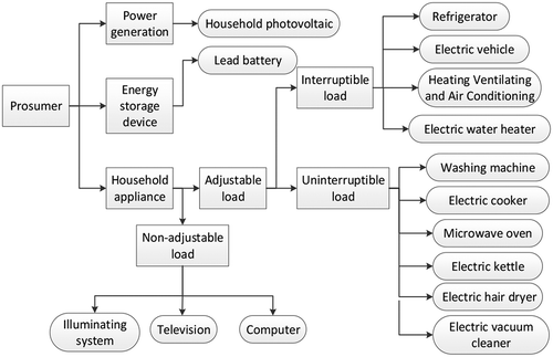
Finally, the household appliances can be divided into flexible load and rigid load, of which the flexible load can be divided into interruptible load and uninterruptible load. The classification of prosumer household appliances is shown in Figure 1.

Figure 1. Component and household appliances classification of Prosumer

The discretisation method is used to model the household appliances. Through the method, aday is divided into nperiods. Yang etal. (2018) establishes the basic model of appliances.

$\sum _{t=1}^n{S}_a(t)=d_a$

$S_a(t)=\left\{\begin{array}{c}\{0,1\},t\in \left[{\alpha }_a,{\beta }_a\right]\\ 0,t\in \left[1,{\alpha }_a-1]\cup [{\beta }_a+1,n\right]\end{array}\right.$

$E_a=P_a\times d_a$

Where S_a(t) is astate variable indicating whether the device a operates during the tperiod; the operation is 1 means working, otherwise it is 0; d_a represents the actual number of time period required for the operation of the device a; [α_a,β_a] is the upper and lower limit of working time for device a; E_a represents the total power consumption of device ain oneday; P_a represents rated power per unit time of device a.

2.1. Uninterruptible load model

Uninterruptible load is the result-oriented load such as washing machine and electric cooker, which means that users will be very uncomfortable if they are interrupted in the middle. This means that once they start using it, they must keep it for acertain period of time. Because the peak load of household users often occurs when using high-power electrical appliances at the same time, and the use time of these high-power loads is schedulable, so it is of great significance to adjust the start time of uninterrupted load flexibly. We set up an uninterruptible load model as follows.

$\begin{array}{rl}& \sum _{t=\tau +1}^{\tau +d_a}{S}_a(t)\ge d_a\cdot \left[S_a(\tau +1)-S_a(\tau )\right]\\ & \tau \in \left[{\alpha }_a-1,{\beta }_a-d_a\right]\end{array}$

Where S_a (t) is 0–1 state variable, indicating the working state of device ain tperiod; d_a is the number of time periods required for adevice ato use electricity; interval [α_a −1,β_a-d_a] is the working time range of adevice a.

2.2. Interruptible load model

Interruptible load refers to the load that does not need continuous power consumption, which can be divided into two categories. One is the temperature-related load, such as HVAC, household refrigerator. The other is the short-term power-off load that needs to be charged/used before the scheduled use time, such as electric vehicle and electric water heater. Therefore, we establish the interruptible load model as follows:

$\sum _{t=\tau +1}^{{\beta }_a}{S}_a(t)=d_a,\tau \in \left[{\alpha }_a-1,{\beta }_a-d_a\right]$

For temperature-related loads such as HVAC, which affect the user’s feeling, the additional constraints to be met are as follows. The HVAC system satisfies the following equality constraints (Liu etal. 2016;Yu etal. 2013)

$J_{ci}=\left\{\begin{array}{c}0,T^{ci}\ge T_{i\mathrm{\_}max}\\ \frac{(T^{ci}-T_{\mathrm{i}\mathrm{\_}min})\cdot (T^{ci}-T_{\mathrm{i}\mathrm{\_}max})}{(T_{i\mathrm{\_}set}-T_{\mathrm{i}\mathrm{\_}min})\cdot (T_{i\mathrm{\_}set}-T_{\mathrm{i}\mathrm{\_}max})},T_{i\mathrm{\_}min}<T^{c\mathrm{i}}<T_{i\mathrm{\_}max}\\ 0,T^{c\mathrm{i}}\le T_{i\mathrm{\_}min}\end{array}\right.$

$T_{ac\mathrm{\_}min}(t)\le T_{ac}(t)\le T_{ac\mathrm{\_}max}(t),i=1,2,\cdot \cdot \cdot ,n$

Where T^ac(t) is the indoor temperature in tperiod; T^out(t) is the outdoor temperature in tperiod; H_a(t), R_a and C_a are the operating thermal power, room thermal resistance and room thermal capacity of air conditioning respectively; T_{ac_min} and T_{ac_max} respectively represent the temperature boundary value of the HVAC.

2.3. Non-adjustable load

There are still some loads in the home which have relatively fixed use time and can not be shifted. Such as lights, televisions, computers etc. In this paper, these loads are considered to be rigid loads expressed by the load prediction curve. Asmall amount of random loads are added on the basis of load forecasting curves. The load forecasting curves are introduced in the form of probability.

3. Users’ comfort with price-sensitive evaluation index

3.1. Construction and consistency of users’ comfort evaluation indicators

Thermal comfort is added to the objective function of household energy management as an evaluation index. Fanger and Toftum (2002) proposed the predictive average voting (PMV), which represents the comfort of most people in the environment. PMV index, which includes four environmental factors of temperature, humidity, wind speed and radiation temperature, and two non environmental factors of human metabolism rate and clothing insulation, has been widely recognised and applied. In terms of PMV index, indoor temperature is the main index affecting human thermal comfort, which is anonlinear function of temperature. In order to transform the problem into amixed integer programming problem, the user’s comfort function is represented by subsection fitting. The structure of comfort index is as follows:

$J_c=\frac{1}{T}\sum _{t=1}^T{J}_c(t)$

$\begin{array}{rl}& J_c(t)=\sum _{i=1}^n{J}_{ci}\cdot {\delta }_i(t)\\ & \sum _{t=1}^T{\delta }_i(t)=n_i\end{array}$

$J_{ci}=\left\{\begin{array}{c}0,T^{ci}\ge T_{i\mathrm{\_}max}\\ \frac{(T^{ci}-T_{\mathrm{i}\mathrm{\_}min})\cdot (T^{ci}-T_{\mathrm{i}\mathrm{\_}max})}{(T_{i\mathrm{\_}set}-T_{\mathrm{i}\mathrm{\_}min})\cdot (T_{i\mathrm{\_}set}-T_{\mathrm{i}\mathrm{\_}max})},T_{i\mathrm{\_}min}<T^{c\mathrm{i}}<T_{i\mathrm{\_}max}\\ 0,T^{c\mathrm{i}}\le T_{i\mathrm{\_}min}\end{array}\right.$

Where J_c represents the comfort evaluation index of temperature-related appliance during time period T; J_ci represents the comfort value of the i-th segment temperature-related appliance. δ_i is a0–1 variable, and 1 indicates that the temperature-related appliance iis on; n_i indicates the required time period of electrical appliance iuse; T^ci is the actual temperature, T_{i_max} and T_{i_mit} are the maximum and minimum value of acceptable comfort zone temperature, T_{i_set} indicates the set temperature value.

3.2. Membership function of the objective function

Generally, just Pareto optimisation sets can be obtained for multi-objective optimisation problems. The fuzzy theory is used to obtain the optimal compromise solution. In the calculation of household energy costs, the goal is to minimise the objective function, which is expressed by the larger fuzzy membership function. The closer the total cost of household electricity is to the minimum, the smaller the objective function value is. So there are:

$\bar{C}=\frac{C-C_{min}}{C_{max}-C_{min}}$

Where: indicates the objective function value of the total cost of household electricity; Cindicates the total cost of household electricity. C_max and C_min respectively represent the maximum and minimum values of the total cost of household electricity.$\bar{C}$

In the calculation of thermal comfort, the goal is to maximise thermal comfort. The smaller fuzzy membership function is selected to minimise the value of the objective function. The closer the value of the fuzzy satisfaction function is to 1, the larger the value of the objective function is. So there are:

$\overline{J_c}=\frac{J_{c\mathrm{\_}max}-J_c}{{J_{c\mathrm{\_}}}_{max}-{J_{c\mathrm{\_}}}_{min}}$

Where indicates the objective function value of thermal comfort; $\overline{J_c}$J_{c_max} and J_{c_min} respectively indicate the maximum and minimum values of thermal comfort.

By constructing the comfort index and price index based on the comprehensive evaluation method, the dimensionless comprehensive evaluation index is realised.

3.3. Comfort target with price-sensitive factor

The current multi-objective optimisation research on HEMS mainly adds each target in the control system simply, and lacks consideration of the intrinsic relationship between the objective functions and its dynamic characteristics. This paper introduces the price-sensitive factor into the fuzzy membership function of thermal comfort, and proposes aprice sensitive home energy management system (PSHEMS). The price-sensitive factors set in this paper are as follows.:

$K_f(t)=\frac{1}{op(t)}$

Where K_f (t) is the price-sensitive factor; op(t) is the real-time price of power grid.

The price-sensitive factor indicates the relative price of the current electricity price. Through the constraint of objective function, the temperature-controlled electrical equipment can be dynamically adjusted according to the change of time-sharing price. The higher the electricity price, the smaller the price-sensitive factor, while the larger the objective function of thermal comfort. Conversely, the lower the electricity price, the smaller the objective function of thermal comfort. Since the goal is the minimum value of the objective function, household energy management is more inclined to arrange more electricity for low-price periods. In general, the period of high price is at the peak of electricity consumption, while the period of low price is at the trough of electricity consumption. In this paper, price-sensitive factor is added to further achieve peak-shaving and valley-filling of the power load under the premise of ensuring comfort and economy.

From Formula (10) and Formula (15), the objective function of comfort function based on the price sensitivity can be revised as following:

$\overline{J_c}=\frac{J_{c\mathrm{\_}max}-\frac{1}{T{K}_f}\sum _{t=1}^T{K}_f(t)J_c(t)}{{J_{c\mathrm{\_}}}_{max}-{J_{c\mathrm{\_}}}_{min}}$

$K_f=\sum _{\mathrm{t}=1}^T{K}_f(t)$

In order to measure the influence of PSHEMS on peak load curve, Peak-to-Average Power Ratio (PAPR) of load curve is considered. Reducing PAPR is also the goal of the power grid, which directly affects the power cost and user comfort.

4. Multi-objective optimisation based on Pareto optimisation

4.1. The objective function of multi-objective optimisation

The optimisation goal of HEMS is to achieve the double optimisation of the user’s comfort and the total operating cost of afamily, so it is amulti-objective optimisation problem. However, the user’s comfort and the total operating cost of afamily belong to different dimensions that are not commensurable. The total objective function cannot be asimple addition of two objectives. Because of the negative correlation between the two objective functions, this paper uses Pareto optimisation to realise the transformation from multi-objective function to single-objective function by setting weight coefficients. The objective function is set as:

$F=min\left\{\left.{\lambda }_1\cdot \bar{C}-{\lambda }_2\cdot \overline{J_c}\right\}\right.$

${\lambda }_1+{\lambda }_2=1$

Where: λ₁ and λ₂ are weight coefficients, which represent the importance of each to the overall objective function. And they can be set different by users according to the different electricity consumption habits. Because the degree of attention has subjective characteristics, this paper adopts the method of assignment based on vague description, as shown in Table 1.

Table 1. Assignment method with vague description

Vague description	Assignment[λ1, λ2]
Cis as important as J	[0.5, 0.5]
Cis slightly more important than J	[0.6, 0.4]
Cis obviously more important than J.	[0.7, 0.3]
Cis much more important than J	[0.8, 0.2]
Cis extremely more important than J	[0.9, 0.1]

The total household operating costs include household electricity purchase cost, storage battery depreciation cost, photovoltaic total electricity subsidy income and household electricity sales income. As follows:

$C=\sum _{t=1}^T\left\{\begin{array}{c}op(t)P_{gb}(t)-psp(t)P_{pv}(t)-sp(t)P_{gs}(t)\\ +{\beta }_b(P_{b.ch}(t)+P_{b.dis}(t))\end{array}\right\}$

Where P_gb(t) and P_gs(t) represent the power purchased from the grid and the power sold to the grid in the tperiod; P_pv(t) is the photovoltaic power in the tperiod; P_b.ch(t) and P_b.dis(t) represent the charging power and discharging power of the stored energy respectively; op(t) represents the power purchase price of the grid; psp(t) is the subsidised electricity price for photovoltaic power; sp(t) is the price of photovoltaic grid-connected electricity; β_b is the depreciation coefficient of battery charge or discharge.

4.2. Power constraints of household nano-grid

Based on the forecasting data, the household nano-grid optimises the charge and consumption of electricity of ESS, HVAC and EV in each period of time and the power consumption time of shifting load in the time-of-use price environment. The constraints of the system are as follows:

(i) Power balance of household nano-grid system:

$P_{gb}(t)+P_{pv}(t)+P_{b.dis}(t)=P_{gs}(t)+P_{b.ch}(t)+P_{ev}(t)+H_a(t)+P_{load}(t)$

Where P_load (t) is the average power of the predicted rigid load in tperiod, H_a (t) is the power consumption of HVAC. P_gb(t) and P_gs(t) represent the power purchased from the grid and the power sold to the grid in the tperiod; P_pv(t) is the photovoltaic power in the tperiod; P_b.ch(t) and P_b.dis(t) represent the charging power and discharging power of the stored energy respectively

(ii) State of charge and charge-discharge power limitation of batteries are as Formula (1), Formula (3)–Formula (9).

(iii) Electric vehicle’s controlled interval of time and full power constraint:

$\sum _{{\alpha }_{ev}}^{{\beta }_{ev}}{S}_{ev}(t)\cdot P_{n.ev}\cdot \mathrm{\Delta }t=E_{ev}$

$E_{ev}=\frac{M}{100}\cdot s\cdot {\int }_0^{+\mathrm{\infty }}{f}_D(r)dr$

Where α_ev and β_ev are respectively the starting and ending time of the charging period of the electric vehicle; S_ev(t) represents the state of charge of the electric vehicle. P_n.ev represents the rated charging power of electric vehicles; E_ev represents the expected amount of charging power required for theday, which can be obtained from the daily driving mileage and probability density function; represents electricity consumption of 100 kilometres. In the following simulation, the charging demand is simulated by randomly generating the daily driving mileage of the vehicle. $M$

(iv) Constraints of power purchase and sale:

$0\le P_{gb}(t)\le P_{gb.max}$

$\left\{\begin{array}{c}0\le P_{gs}(t)\le P_{pv}(t)\\ 0\le P_{gs}(t)\le P_{gs.max}\end{array}\right.$

Where P_gb.max and P_gs.max represent the limit of purchasing and selling power of household nanogrid respectively.

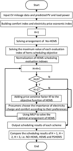
4.3. MILP Model solving process

We consider three types of household energy allocation, regardless of HEMS, HEMS based on Pareto equilibrium and improved price-sensitive HEMS (PSHEMS). In order to better evaluate the quality of dispatching results, three indicators of customer comfort, cost and PAPR of power grid are evaluated. In the optimised scheduling scheme, in addition to comprehensive consideration of cost and comfort, we also give users acertain choice, and customers can choose the importance level of cost and comfort according to their own preferences. In addition, it is difficult to determine the weight of the comfort index for different loads at different periods when determining the comfort optimisation target. To this end, for the dispatchable load of air conditioners etc, price sensitivity factors are introduced into the comfort model to construct avirtual comfort based on unitised electricity prices. This associates comfort and cost according to the electricity price to further reduce the cost while ensuring comfort. The specific solution process is shown in Figure 2.

Figure 2. Flow chart of solving model

5. Example analysis

5.1. Parameter settings

5.1.1. Load parameters

Several common household loads set up in this paper are shown in Table 2.

Table 2. Household appliances parameters

Name of household appliances	Rated power (kW)	Working interval	Working hours (h)	Minimum continuous working hours (h)
Washing machine	1	12:00–23:00	0.75	0.75
Electric cooker	0.8	6:00–7:0010:00–12:0016:00–18:00	3	1
Microwave oven	1	17:00–18:00	0.5	0.5
Vacuum cleaner	0.8	18:00–22:00	0.5	0.25
Electric kettle	1.2	7:00–9:0017:00–18:00	0.5	0.25
Air blower	1.2	21:00–23:00	0.25	0.25
Electric vehicle	6.3	19:00–7:00 the nextday	/	/
HVAC	2	19:00–6:00the nextday	/	/

Among them, the Nissan Leaf form is considered for household EV, of which the on-board battery capacity is 24 kW⋅h. According to Chaudhari etal. (2019), the charging power of slow charging mode is P_n.ev = 6.3 kW. It is mainly used to meet the travel demand, so discharge to power grid EV is not considered. The charging time of the electric vehicle set in this paper is 19:00 ~ 7:00 the nextday. The number of required charging periods is obtained according to the daily driving mileage sand its probability function. And based on Pourmousavi, Patrick, and Nehrir (2014) research, the power consumption of 100 kilometres is 15 kWh/kM.

The working time of HVAC is set from 19:00 to 6:00 the nextday. The room thermal capacity is C_a = 0.525 kW⋅h/°C; the room thermal resistance is R_a = 16°C/kW; the comfort range after air conditioning is turned on is T_min = 23°C, T_max = 28 °C; the rated power of air conditioning is P_aN = 2 kW.

5.1.2. PV, energy storage and price parameters

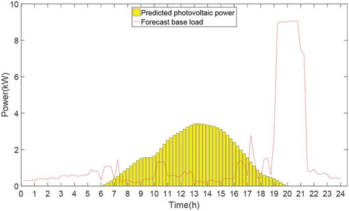
In this paper, three-point method is used to forecast photovoltaic power generation. Firstly, solar radiation is obtained according to weather forecast, and then the forecast value of photovoltaic power generation is obtained. The PV obtained from weather forecast and the predicted load in mid summer in July in Guangdong are shown in column diagram of Figure 3. It shows that the household load without HEMS is concentrated between 19:00 and 22:00, which is the peak load period. It is different from the photovoltaic generation curve.

Figure 3. Predicting photovoltaic power and load

For the choice of household batteries, this paper adopts the battery whose parameters are shown in Table 3.

Table 3. Household batteries

Capacity	SOCmin	SOCmax	Pch/Pdisch	ηloss	ηself
4 kW⋅h	0.1	0.9	3 kW	5%	2%

The time-of-use price scheme in Guangzhou is adopted for power grid price. The grid price, PV on-grid tariff and photovoltaic electricity subsidised price are shown in Table 4.

Table 4. Electricity price in Guangzhou (yuan/kWh)

Classification	Time frame	Purchase price	Sale price	Subsidise price
Peak period	14:00 ~ 17:0019:00 ~ 22:00	0.96	0.34	0.18
Flat period	8:00 ~ 14:0017:00 ~ 19:0022:00 ~ 24:00	0.58	0.34	0.18
Valley period	0:00 ~ 8:00	0.29	0.34	0.18

5.2. Simulation results

5.2.1. Analysis of PSHEMS optimisation results

When the weight of total cost and user’s comfort is set to 0.3/0.7, combining with forecasting the power and load of photovoltaic power generation, the price-sensitive HEMS is used to get theday-ahead planning of household energy. Figure 3. shows the daily effect curve of HEMS, which reflects the residential energy management with the consideration of power grid, renewable energy, battery storage and electric vehicle.

Figure 4. PSHEMS effect curve for oneday

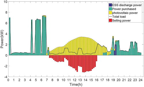
Comparing Figures 3 and 4, from the user side, PSHEMS transfers the load of peak period at 19:00–22:00 to valley period at 0:00–6:00, which helps to reduce household cost. From the grid side, the load is transferred from peak period to non-peak period, which realises the optimal allocation of load and improves the overall load characteristics. Although load transfer smoothes load curve and reduces user cost, it may interfere with user comfort.

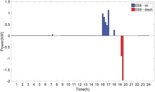
The charging and discharging power of energy storage under PSHEMS is shown in Figure 5. PSHEMS charged the energy storage device at 16:00–18:00 when photovoltaic power generation was sufficient. The energy storage device is used to supply power during the peak period at 19:00–20:00. It shows that certain energy storage equipment can transfer renewable energy, so as to provide more electricity for families during peak period, and realise the optimal configuration of power supply.

Figure 5. Energy storage charge and discharge power

In conclusion, the PSHEMS proposed in this paper can improve the utilisation of renewable energy and optimise the load consuming time by optimising the allocation of household load and power supply. As aresult, the operating cost of the entire dispatching cycle is reduced and the load characteristic curve of power grid is smoothed.

5.2.2. Comparison of energy management in different families

Different household energy management methods, which are NO-HEMS, HEMS and PSHEMS, are considered. Among them, HEMS and PSHEMS adopt the hybrid Integer programming algorithms based on fuzzy control to realise the Pareto optimisation of the multi-objective optimisation.

When the weight of total cost of household operation and user comfort is set to 0.3/0.7, the system will adopt three kinds of household energy management: NO-HEMS, HEMS and PSHEMS. In order to visualise the peak, flat and valley periods of electricity price, it is synchronously displayed in Figure 5.

Figure 6. The purchase of electricity in the summer household nano-grid system under various operating modes

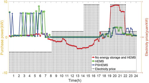
As shown in Figure 6, HEMS transfers the load of 19:00–22:00 in peak period to 0:00–8:00 in valley period to save cost; PSHEMS further transfers the load of 19:00–22:00 in peak period arranged by HEMS to 22:00–24:00, in normal period, which further reduces the cost of electricity consumption and smoothes the load curve.

When NO-HEMS, HEMS and PSHEMS are used in the system, the daily expenditure, income, comfort and PAPR are calculated, which are shown in Table 5.

Table 5. Cost, benefit, user comfort and PAPR in different modes

Mode	Expenditure(yuan)	Income(yuan)	Comfort(pu)	Peak-to-average power ratio (pu)
No energy storage, no HEMS	28.15	10.06	0.89	13.22
Considering HEMS	14.94	10.06	0.81	4.74
PSHEMS	13.41	10.06	0.81	3.95

Table 5 shows that household daily expenditure can be reduced by 47% with HEMS, which is further reduced by 53% with PSHEMS. After using HEMS and PSHEMS, the household income did not change, but the user comfort was both reduced by 9%. At the same time, the PAPR value of daily load curve can be reduced by 64% and 70% after using HEMS and PSHEMS. On the premise of guaranteeing the user’s comfort and electricity revenue, the proposed PSHEMS reduces the PAPR value of the user’s expenditure and load curve properly on the basis of HEMS.

5.2.3. Comparison of the changes of the weight of objective function

When the weight λ₁/λ₂ of objective function changes, the daily household expenditure, income, comfort and PAPR of PSHEMS under different weights can be calculated, which are shown in Figure 7.

Figure 7. Income, cost and PAPR of load curve under different weights of the system objectives

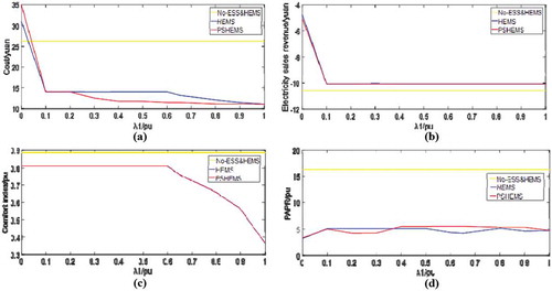
Figure 7 shows the household expenditure, income, comfort and peak load curve average with different household energy management methods when the weight λ₁ of total household operating cost in the objective function changes from 0.1 to 1. It shows that compared with NO-HEMS, when HEMS and PSHEMS are used in the system, household expenditure and PAPR value decrease significantly, while income decreases slightly. The comfort degree of using HEMS and PSHEMS is slightly lower than that of NO-HEMS when λ₁ is smaller, 0.1–0.6. When λ₁ is larger, that is, the weight of family total cost is larger, the comfort degree of HEMS and PSHEMS decreases with the increase of λ₁.

Compared with ordinary HEMS, PSHEMS has afurther reduction in household expenditure with the same income and comfort, and no obvious advantage in PAPR.

The results further verify that PSHEMS and HEMS can effectively reduce the user’s expenditure and PAPR of load curve on the premise of guaranteeing user’s income and comfort. PSHEMS can further reduce user spending on the basis of HEMS optimisation. However, PSHEMS has no obvious advantage over HEMS in reducing PAPR of load curve. On the other hand, although the PSHEMS calculation results are slightly different with different weights, it will not have agreat impact on the trends and changes of household expenditure, income, comfort and PAPR values.

6. Conclusion

In this paper, aprice sensitive household energy management method based on Pareto optimisation is proposed. Firstly, according to the characteristics of different household appliances, the user equipment is classified and modelled. Considering the negative correlation between user power consumption and comfort, the weighted Pareto optimisation is used to solve the objective function. Different from the existing home energy management algorithm, this method also adds price sensitive factor to the membership function of the objective function, and uses the MILP to solve this problem. The results show that the scheme can not only ensure the comfort of home users, but also reduce the power cost of home users more effectively. In other words, it has more economic advantages than the general energy management method. However, there is still something to be improved in this study: the prediction is always wrong. In this case, the huge potential of energy storage peak cutting and valley filling to generate additional income is caused by unforeseen large peaks, but it is not necessarily the case. The load demand will deviate from the forecast in the future, so the optimal scheduling result of this paper is actually suboptimal. The economic benefit of energy storage system applied to asingle family is relatively limited compared with its cost, and according to the scheduling results, the main events of energy storage are concentrated in the peak load period, and the utilisation rate of other periods is not high. It may be aworthy research direction to consider the situation of multiple prosumers sharing energy storage.

Disclosure statement

No potential conflict of interest was reported by the authors.

Additional information

Funding

This work was supported by the National Natural Science Foundation of China [51607093].

Notes on contributors

Jie Lyu

Jie Lyu, female, received the B.Eng. degree in electrical engineering from North China Electric Power University, Beijing, China, in 2016. Currently, she is pursuing the M.S. degree in electrical engineering at Nanjing Normal University, Nanjing, China. Her research interests include renewable power generation, power system analysis and demand side response

Tairan Ye

Tairan Ye, male, is currently studying for a Bachelor of Electrical Engineering degree at Nanjing Normal University.

Mengtian Xu

Mengtian Xu, female, is currently studying for aBachelor of Electrical Engineering degree at Nanjing Normal University.

Gang Ma

Gang Ma*, male, received the Ph.D.degree in electrical engineering from North China Electric Power University in 2013 and is presently an associate professor in School of Electrical & Automation Engineering, Nanjing Normal University, Nanjing, China. His current research interests include renewable energy generation and grid-connected technology.

Ying Wang

Ying Wang, female, graduated from Southeast University with abachelor’s degree, and she is pursuing the M.S.degree in electrical engineering at Nanjing Normal University, Nanjing, China.

Mengyue Li

Mengyue Li, female, graduated from Southeast University with abachelor’s degree, and she is pursuing the M.S.degree in electrical engineering at Nanjing Normal University, Nanjing, China.

References

- Rathnayaka,A.J., P.Dinusha, M.Vidyasagar, O.Hussain, and T.S. Dillon. 2011. International Conference on Cloud & Service Computing. IEEE Computer Society.Identifying Prosumer’s Energy Sharing Behaviours for Forming Optimal Prosumer-communities. doi:10.1109/CSC.2011.6138520.
- Kobus,C., R.Mugge, and J.P.L. Schoormans. 2015. “Long-term Influence of the Design of Energy Management Systems on Lowering Household Energy Consumption.” International Journal of Sustainable Engineering 8 (3): 173–185. doi:10.1080/19397038.2014.991776.
- Melhem, F.Y., O.Grunder, Z.Hammoudan, and N.Moubayed. 2017. “Optimization and Energy Management in Smart Home considering Photovoltaic, Wind, and Battery Storage System with Integration of Electric Vehicles.” Canadian Journal of Electrical & Computer Engineering 40 (2): 128–138.
- Shareef,H., M.S. Ahmed, A.Mohamed, and E.Al Hassan. 2018. “Review on Home Energy Management System considering Demand Responses, Smart Technologies, and Intelligent Controllers.” IEEE Access 6: 24498–24509.
- Joo, I.Y., and D.H.Choi. 2017. “Optimal Household Appliance Scheduling considering Consumer’s Electricity Bill Target.” IEEE Transactions on Consumer Electronics 63 (1): 19–27. doi:10.1109/TCE.2017.014666.
- Yang,J., J. Liu, Z.Fang, and W.Liu. 2018. “Electricity Scheduling Strategy for Home Energy Management System with Renewable Energy and Battery Storage: ACase Study.” IET Renewable Power Generation 12 (6): 639–648. doi: 10.1049/iet-rpg.2017.0330.
- Chaudhari,K., N.K. Kandasamy, A.Krishnan, A.Ukil, and H.B.Gooi. 2019. “Agent-Based Aggregated Behavior Modeling for Electric Vehicle Charging Load.” IEEE Transactions on Industrial Informatics 15 (2): 856–868. doi:10.1109/TII.2018.2823321.
- Collotta,M., and G.Pau. 2015. “ANovel Energy Management Approach for Smart Homes Using Bluetooth Low Energy.” IEEE Journal on Selected Areas in Communications 33 (12): 2988–2996. doi:10.1109/JSAC.2015.2481203.
- Faruque, M.A.A., and K.Vatanparvar. 2015. “Energy Management-as-a-service over Fog Computing Platform.” IEEE Internet of Things Journal 3 (2): 161–169. doi:10.1109/JIOT.2015.2471260.
- Erdinc,O., N.G. Paterakis, T.D.P. Mendes, A.G. Bakirtzis, and P.S.C.Joao. 2015. “Smart Household Operation considering Bi-directional Ev and Ess Utilization by Real-time Pricing-based Dr.” IEEE Transactions on Smart Grid 6 (3): 1281–1291. doi:10.1109/TSG.2014.2352650.
- Nyeng,P., and J.Ostergaard. 2011. “Information and Communications Systems for Control-by-Price of Distributed Energy Resources and Flexible Demand.” IEEE Transactions on Smart Grid 2 (2): 334–341. doi:10.1109/TSG.2011.2116811.
- Rajendhar,P., and B.E. Jeyaraj. 2019. “Application of DR and Co-simulation Approach for Renewable Integrated HEMS: A Review.” IET Generation, Transmission & Distribution 13 (16): 3501–3512. doi:10.1049/iet-gtd.2018.5791.
- Fanger, P.O., and J.Toftum. 2002. “Extension of the Pmv Model to Non-air-conditioned Buildings in Warm Climates.” Energy and Buildings 34 (6): 533–536. doi:10.1016/S0378-7788(02)00003-8.
- Xu, Q.S., H.X. Zang, and H.H. Bian. 2011. “Establishment and Feasibility Researches of Practical Solar Radiation Model.” Acta Energiae Solaris Sinica 32 (8): 1180–1185. (in Chinese).
- Zafar,R., A.Mahmood, S.Razzaq, W.Ali, U.Naeem, and K.Shehzad. 2018. “Prosumer Based Energy Management and Sharing in Smart Grid.” Renewable & Sustainable Energy Reviews IEEE 82: 1675–1684. doi:10.1016/j.rser.2017.07.018.
- Hu, R.L., R.Skorupski, R.Entriken, and Y.Ye. 2016. “A Mathematical Programming Formulation for Optimal Load Shifting of Electricity Demand for the Smart Grid.” IEEE Transactions on Big Data. doi:10.1109/TBDATA.2016.2639528.
- Aznavi,S., P.Fajri, A.Asrari, and F.Harirchi. 2020. “Realistic and Intelligent Management of Connected Storage Devices in Future Smart Homes considering Energy Price Tag.” IEEE Transactions on Industry Applications 56 (2): 1679–1689. doi:10.1109/TIA.2019.2956718.
- Pourmousavi,S.A., S.N.Patrick, and M.H.Nehrir. 2014. “Real-time Demand Response through Aggregate Electric Water Heaters for Load Shifting and Balancing Wind Generation.” IEEE Transactions on Smart Grid 5 (2): 769–778.
- Shafie-Khah,M., and P.Siano. 2017. “AStochastic Home Energy Management System considering Satisfaction Cost and Response Fatigue.” IEEE Transactions on Industrial Informatics PP (99): 1-1.
- Liu,Y., Y.Zhang, K.Chen, S.Z. Chen, and B.Tang. 2016. “Equivalence of Multi-time Scale Optimization for Home Energy Management considering User Discomfort Preference.” IEEE Transactions on Smart Grid 1-1. doi:10.1109/TSG.2016.2545683.
- Wu,Z., S.Zhou, J.Li, and X.P. Zhang. 2014. “Real-time Scheduling of Residential Appliances via Conditional Risk-at-value.” IEEE Transactions on Smart Grid 5 (3): 1282–1291. doi:10.1109/TSG.2014.2304961.
- Yu,Z., L.Jia, M.C. Murphy-Hoye, A.Pratt, and L.Tong. 2013. “Modeling and Stochastic Control for Home Energy Management.” IEEE Transactions on Smart Grid 4 (4): 2244–2255. doi:10.1109/TSG.2013.2279171.