An imperfect production model with energy consumption, GHG emissions and fuzzy demand under a sustainable supply chain

ABSTRACT

In this article, an integrated two-level supply chain model is described in two different scenarios by treating the demand rate as a triangular fuzzy number. In the first scenario, the retailer offers a price discount for customers on the backorders; it encourages the customer to wait for the product. In the second scenario, the retailer does not provide any discount; instead, an investment is made to reduce lost sales during the stock-out. In both scenarios, the shortages are allowed, and it is partially back-ordered. Two different cases are discussed within these scenarios with two different production functions related to the process quality and production rate. The signed distance method is employed to handle the fuzzified parameter. This research aims to minimize the total expected cost of the supply chain model under each scenario with energy consumption and greenhouse gas emissions during the production process. Moreover, to investigate how changes in the production rate affect the quality of products produced and the entire model’s total cost under the effects of backorder price discounts and lost sales reduction. An iterative algorithm is followed to acquire numerical results. To demonstrate the model, some numerical instances, sensitivity analysis and managerial insights are provided.

KEYWORDS:

• Energy consumption
• fuzzy demand
• imperfect production
• lost sale reduction
• transportation
• variable backorder

1 Introduction

Over the years, industries and manufacturing companies have been releasing various pollutants into the environment through land, air and water. It is estimated that about 50 per cent of all pollution is caused by industrial and manufacturing activities. It reveals that industries also play an essential role in delivering harmful and hazardous pollutants to the environment. Furthermore, diseases, loss of life and environmental degradation are the effects of pollution. This pollution has been proven to be extremely harmful to the environment in several forms. Moreover, in industry, energy is used in many ways, i.e. most businesses or organizations use energy during the production phase for several processes. In general, electrical energy, steam energy, and cooling energy are the energy used by companies. So there are costs involved in operating and purchasing these systems. Therefore, it seems necessary to consider the need for energy. It requires both electricity and workforce during the production process, so we incorporate the cost of energy use during the production and rework of defective materials. Greenhouse gas (GHG) absorb energy and warm the earth. Human activities have been mainly responsible for increasing greenhouse gases in the atmosphere over the past 150 years.

In any industry, the production rate is not always balanced, and it keeps changing concerning the situations. Also, if the product’s demand is high among the consumers, the company will increase production rate. Similarly, as the demand for a product decreases, so does the rate of production. Therefore, it is good to consider the variable production, which is one of the realistic factors. Suppose there is any problem with the production machinery during the production phase. In that case, the machine shift from the in-control position to the out-of-control position, so the resulting product will be defective, leading to the imperfect production process.

It is difficult for a company to predict its demand rate before marketing, so the demand for goods in the market may be low or high. Based on this, it is evident that the market demand for a product cannot be constant; that is, the demand rate is unclear. In this stage, the requirement for the product is said to be an uncertain demand. The demand uncertainty occurs when a business or an industry cannot accurately predict consumer demand for its products or services. The fuzzy logic techniques effectively solve complex, ill-defined problems characterized by environmental uncertainty and ambiguity of information. It allows for handling uncertain and imprecise knowledge and provides a robust framework for reasoning. Therefore, it has been confirmed that fuzzy logic is compelling in overcoming such uncertainty, and it describes a phenomenon in which a mathematical model or input data is unknown. Thus, the solution to these sorts of challenges can be found by considering an uncertainty parameter with a fuzzy number. In our model, the product’s demand rate holds the uncertainty, and to treat this, we consider a triangular fuzzy number.

Consequently, in this model, we will look at how the industry affects the environment and how to reduce overall costs by mitigating these impacts.

2 Literature review

This subsection describes the detailed review analysis of the existing literature works.

2.1 Energy consumption and GHG emission

Over time, industries emit more and more greenhouse gases, especially as the production process increases, resulting in more greenhouse gas emissions. Plambeck (2012) has described the experience of the world’s largest business and how it can reduce GHG emissions in the supply chains of start-ups and offer suggestions for expanding the efficiency of new zero-emission supply chains. By considering GHG emissions from manufacturing processes and various carbon trading systems, Jaber et al. (2013) have developed a two-stage supply chain model with a collaborative framework, proposing possible combinations between these projects. Bazan et al. (2015) explained two models, typically considering the energy used in the manufacturing process from a single seller to a single buyer under consignment stock policy. Ugarte et al.(2016) presented a supplier-retailer supply chain model by incorporating the cost for GHG emissions during the production process and analysed the profit functions of decentralised and centralised models with the sense of emissions trading schemes. Sarkar et al. (2018) have developed a supply chain manufacturing model with suppliers for the automobile parts manufacturing industry to improve production volume with multiple objectives, mainly by reducing energy costs while considering renewable energy. With better energy policy and energy consumption, Safarzadeh and Rasti-Barzoki (2019) discussed share price decisions to increase the profitability of supply-chain players. Karthick and Uthayakumar (2021) developed a multi-item inventory model with CS policy to reduce the carbon emission through the logarithmic investment.

2.2 Imperfect manufacturing process

In the literature, many researchers had described imperfect production models. Imperfect production is caused due to mechanical errors in the manufacturing process. Rosenblatt and Lee (1986) examined the effects of imperfect manufacturing processes on deteriorating goods during the optimum production cycle. Cheng (1991) proposed an EOQ model with demand-oriented unit manufacturing cost under the imperfect manufacturing processes. Salameh and Jaber (2000) have illustrated a production inventory model by considering the manufacturing process in perfect and imperfect situations. Hayek and Salameh (2001) have examined the impact of defective quality products on a limited production scale and predicted that faulty products to rework at a constant rate. Liao et al. (2009) developed comprehensive maintenance and improvement plans with an EPQ model for an incomplete process, including a deteriorating production system with an increased risk ratio. Sarkar et al. (2011) described an EPQ model for continuous and unique random demand for goods and examines the percentage decrease in overall output with an increase in production run time when the manufacturing process is considered imperfect.

2.3 Sustainable and variable production

Khouja and Mehrez (1994) have illustrated an imperfect production model by considering the production rate as a variable with the quality process. Sarkar et al. (2018) have established an imperfect supply chain model under varying production process with the incorporation of the unit manufacturing cost as a function of the production rate, and analysed the three various production functions correlated with system quality and production rate. Marchi et al. (2019) have developed a two-stage supply chain model that considers two integrated principles: classical and vendor-managed inventory policies, including inventory maintenance costs, GHG emissions, material and process efficiency, and transport operations. Herbon (2020) developed an approximated solution to the constrained integrated supply model by considering the variable production rate.

2.4 Expected shortages and effects of backorder price discount

Shortages can occur when there is not enough inventory. Simultaneously, some customers may switch to other enterprise products, and to overcome this problem, some researchers have proven through their model that they can retain customers by offering price discounts on backorder products. For practical purposes, Gallego and Moon (1993) were first to develop an inventory model, in which the lead time demand doesn’t follow any specific distribution. Subsequently, considering (Gallego and Moon (1993)) model, an inventory model has been developed by Lin (2008) to address the demand for a lead time that does not follow any specific distribution with a backorder price discount. Sarkar et al. (2015) illustrated the concept of an inventory model with a price discount plan, taking into account the initial investment to enhance the quality of the product. Ganesh Kumar and Uthayakumar (2019) have considered a two-level supply chain model with multi-item, variable backorder under trade credit policy.

2.5 Lost sale reduction

In many cases, some customers will not wait for the goods they need in the absence of inventory. In this situation, the manufacturer or seller may lose customers. So some researchers thought lost sale reduction would help such situations. Ouyang and Chang (2001) illustrated a model to analyse the effects of lost sale reduction with the lead time demand to follow normal and free distribution approach. Hwang et al. (2013) developed the economic lot-sizing problem with lost sales and bounded inventory. Soni et al. (2018) have developed an inventory model with lost sale reduction, quality improvement under the fuzzy environment. ElHafsi et al. (2021) examined optimal production and inventory control of multi-class mixed backorder and lost sales demand class models.

2.6 Fuzzy demand

Most researchers consider the demand rate of the product to be uncertain, for instance, Ouyang and Yao (2002), Dutta et al. (2007), Björk (2009), Mula et al. (2010) considers the customers demand to be a fuzzy number. Moreover, Taleizadeh et al. (2013) illustrated the supply chain model by considering the demands as a fuzzy rough variable. Malik and Sarkar (2019) developed an inventory model based on the coordinating system with fuzzy demand and the defuzzification process is made by the signed distance method. Noh and Kim (2019) derived a coordinating supply chain model between a single vendor and multi-buyer by considering the demand as a triangular fuzzy number. Karthick and Uthayakumar (2020) investigated the imperfect production model with a triangular fuzzy demand.

2.7 Research gap and contribution

Contributions of various study articles from the existing literature are given in Table 1. From examining the above subsections, there has been very little research on back-order price discount and lost sales, and no inventory model has been found under the ambiguous/fuzzy context, especially since there is no model to compare these two (i.e., back-order price discount and lost sales) together. And, in particular, it is important to consider the fact that energy consumption and carbon emissions studies are limited in the literature. Of these, to our knowledge, none of the supply chain models has been reported in the literature on the imperfect inventory model with fuzzy demand, energy consumption, GHG emissions under two different scenarios, such as providing a price discount to the customers on the first scenario and in the second scenario, an investment is made in reducing lost sales without offering any discounts.

Table 1. A comparison of the present model with related existing models

Reference	Imperfect production	Fuzzy demand	Defective reworking	Mean Time To Failure	Energy consumption	GHG emission	Variable Production rate	Price discount	Lost sale reduction
Khouja and Mehrez (1994)	✓		✓	✓			✓
Hayek and Salameh (2001)	✓		✓
Ouyang and Yao (2002)		✓
Dutta, Chakraborty, and Roy (2007)		✓
Lin (2008)								✓
Liao, Chen, and Sheu (2009)	✓
Mula, Peidro, and Poler (2010)		✓
Taleizadeh, Wee, and Jolai (2013)		✓						✓
Bazan, Jaber, and Zanoni (2015)					✓	✓
Sarkar, Mandal, and Sarkar (2015)								✓
Sarkar, Omair, and Choi (2018)			✓		✓	✓
Sarkar et al. (2018)	✓		✓	✓			✓
Soni et al. (2018)	✓								✓
Marchi et al. (2019)	✓		✓		✓	✓
Noh and Kim (2019)		✓				✓
Ganesh Kumar and Uthayakumar (2019)	✓							✓
Herbon (2020)							✓
Karthick and Uthayakumar (2021)		✓				✓	✓
Present model	✓	✓	✓	✓	✓	✓	✓	✓	✓

The rest of the paper is given as follows: some basic definitions are given in section 3. In section 4 problem definition, notations and assumptions are given to develop the model. Section 5 contains the mathematical model of both retailer and manufacturer. In section 6–7, an integrated cost function is developed under two scenarios, one is while providing backorder price discounts to the customers and another is while retailer plans to make an investment to reduce lost sale respectively, in which two different cases are considered to relate the production rate and process quality under these scenarios. Moreover, in this paper, the demand rate is considered a triangular fuzzy number and the defuzzification process is done using the signed distance method. Two numerical examples are considered for each scenario to validate this model. Graphical representations are given to illustrate the model. In section 8, sensitivity analysis and managerial implications are given. Finally, the conclusion is given in section 9.

3 Preliminaries

Definition 3.1 (Fuzzy number) A fuzzy number is a fuzzy subset of $\mathbb{R}$ which is both normal and convex. In addition, the membership function must be piece wise continuous. The membership function of a fuzzy number $\tilde{F}$ is usually represented as

(1) ${\mu }_{\tilde{F}}(x)=\left\{\begin{array}{c}{f}_{\iota }(x),x<m\\ 1,m\le x\le n\\ f_u(x),x>n\end{array}\right.$(1)

where, $f_l(x)$ is continuous from the right, strictly increasing for $x<m$ and there exist $m_1$ < m such that $f_l(x)=0$ for $x\le m_1$ and $f_u(x)$ is continuous from the left, strictly decreasing for $x>n$ and there exist $n_1\ge n$ such that $f_u(x)=0$ for $x\ge n_1.$ $f_l(x)$ and $f_u(x)$ are called the left and right reference functions respectively.

Definition 3.2 ($\alpha$ cut of a fuzzy set (Björk 2009)) The set $\tilde{F}(\alpha )=\{x:{\mu }_{\tilde{F}}(x)\ge \alpha \},$ where $\alpha \in [0,1]$ is called the $\alpha$ cut of $\tilde{F}$ $\tilde{F}(\alpha )$ is a nonempty bounded closed interval contained in the set of real numbers and it is denoted by $\tilde{F}(\alpha )=[{\tilde{F}}_L(\alpha ),{\tilde{F}}_U(\alpha )].$ Both ${\tilde{F}}_L(\alpha )$ and ${\tilde{F}}_U(\alpha )$ are continuous functions of $\alpha \in [0,1].$ Let ${\tilde{F}}_L(\alpha )$ and ${\tilde{F}}_U(\alpha )$ are the left and right limits of $\tilde{F}(\alpha )$ respectively, are usually known as the left and right α cuts of $\tilde{F}.$

Definition 3.3 (Triangular fuzzy number (Karthick and Uthayakumar 2020)) The fuzzy number $\tilde{F}$ is a triangular fuzzy number (see, Figure 1) if it is fully determined by $(t_1,t_2,t_3)$ of crisp numbers such that $t_1<t_2<t_3$ with membership function

(2) ${\mu }_{\tilde{F}}(x)=\left\{\begin{array}{cc}L(x)=\frac{x-t_1}{t_2-t_1},& t_1\le x\le t_2\\ R(x)=\frac{t_3-x}{t_3-t_2},& t_2\le x\le t_3\\ 0,& otherwise\end{array}\right.$(2)

Figure 1. Triangular fuzzy number

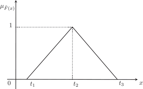
where, $t_1,t_2$ and $t_3$ are the lower limit, mode and upper limit of the fuzzy number. The interval $[t_1,t_3]$ is called the support of the fuzzy number which gives the range of all values that are at least marginally possible or plausible. $t_2$ is known as the core or the most plausible value. For the triangular fuzzy number $\tilde{F}=(t_1,t_2,t_3),$ the left and right α cuts of $\tilde{F}$ are respectively given by ${\tilde{F}}_L(\alpha )=t_1+(t_2-t_1)\alpha$ and ${\tilde{F}}_U(\alpha )=t_3-(t_3-t_2)\alpha .$

Definition 3.4 (Signed distance method (Karthick and Uthayakumar 2020)) For any $t\in R,$ $d_0(t,0)=t$ is named as the signed distance from t to 0. If $t>0,$ then the distance from t to 0 is $t=d_0(t,0);$ if $t<0,$ the distance from t to 0 is $-t=-d_0(t,0).$ Therefore, $d_0(t,0)=t$ is known as the signed distance from t to 0 For the fuzzy set $\tilde{F}\in R^{+},0\le \alpha \le 1,$ the following expression can be obtained as $\tilde{F}={\cup }_{0\le \alpha \le 1}{\tilde{F}}_{\alpha }={\cup }_{0\le \alpha \le 1}[L_{\alpha },R_{\alpha }].$ The signed distance of the interval $[L_{\alpha },R_{\alpha }]$ measured from the origin 0 is given by

(3) $d_0([L_{\alpha },R_{\alpha }],\tilde{0})=\frac{({\tilde{F}}_L(\alpha )+{\tilde{F}}_U(\alpha ))}{2}.$(3)

For the fuzzy number $\tilde{F}\in R^{-},$ the proposed defuzzification methods $d_0(\tilde{F},0)$ (the distance from $\tilde{F}$ to 0) is written as

$d_0(\tilde{F},\tilde{0})={\int }_0^1{d}_0({\tilde{F}}_{\alpha },\tilde{0})d\alpha$

$={\int }_0^1{d}_0([L_{\alpha },R_{\alpha }],\tilde{0})d\alpha$

$=\frac{1}{2}{\int }_0^1\{{\tilde{F}}_L(\alpha )+{\tilde{F}}_U(\alpha )\}d\alpha$

$=\frac{1}{2}{\int }_0^1[t_1+(t_2-t_1)\alpha +t_3-(t_3-t_2)\alpha ]d\alpha$

(4) $=\frac{1}{4}[t_1+2t_2+t_3].$(4)

4 Problem definition, notations and assumptions

4.1 Problem definition

The primary purpose of this article is to examine experimental parameters in two scenarios of a model – (1) when the retailer offers discounts to the customers on the backorders, (2) to minimize the lost sales without offering any discounts and these two scenarios are described by considering uncertain demand, energy consumption for manufacturing and reworking process, greenhouse gas emissions under imperfect production in a fuzzy environment. In fact, many industries speed up their production and increase its volume to deliver products to their customers faster. If there are any defects in the general mechanism during the manufacturing process, it causes the production of defective items, leading to shortages and a lost sale. To reduce the shortage/lost sale, the retailer takes the shortages as a backorder and offers a discount to the customers in the first scenario. Moreover, some customers may accept the backorders, and some may not accept that there may be an occurrence of lost sale in such cases. In the second scenario, if the retailer decided to make an investment for reducing the lost sale may be helpful to attain a minimum total cost without offering any discount. Due to imperfect production, the retailer is unable to deliver the products on time, and as a result, cannot meet the demand of the customers. Therefore, the demand for the product is likely to decrease, but it is impossible to calculate it accurately, which leads to uncertainty. Therefore, in this model, the demand is considered as a triangular fuzzy number. Moreover, under these two scenarios, the lead time demand does not follow any specific distribution but mean, and standard deviation are known.

In this paper, we develop a mathematical model using the notations and assumptions listed below.

4.2 Notations

The following notations will be used to develop the model

Table

Decision variables
$Q_b$	order quantity (units)
k	safety factor
${\pi }_x$	backorder price discount ($/unit)
ρ	lost sale during the fraction of shortage in the stockout period, $0\le \rho \le 1$
P	production rate (units/year)
n	number of shipments, a positive integer
Parameters
D	demand rate (units/year)
$A_v$	setup cost ($/setup)
$A_b$	ordering cost ($/order)
$H_b$	holding cost for the retailer ($/unit/year)
$H_v$	holding cost for the manufacturer ($/unit/year)
R	reworking cost ($/unit)
$\sigma$	standard deviation
r	reorder level
$\tau$	backorder ratio, $0<\tau <1$
${\tau }_0$	upper bound of backorder ratio
${\pi }_0$	marginal profit per unit
T	fixed transportation ($/shipment)
V	variable transportation ($/unit)
$\alpha$	percentage of defective items during the production process in ‘out-of control’ stage
$E_{N_d}$	expected number of defective items produced
$w_p$	idle power for production process (kW)
$w_r$	idle power for reworking process (kW)
$\gamma$	relation between the reworking and production rate
$\eta$	emissions function factor (ton/unit)
$E_c$	GHG emissions tax cost ($/ton)
$W_c$	fixed warrenty cost per unit ($/unit)
$I_c$	fixed inspection cost per unit ($/unit)
${\rho }_0$	initial lost sale
$\pi$	shortage cost ($/unit)
$\xi$	fractional cost of the capital investment per unit per order
$l(Q_b,P)$	length of the lead time

4.3 Assumptions

1. A single-manufacturer single-retailer inventory model is considered with a single type of item.

2. Retailer follows a continuous review inventory system with partial backordering.

3. Manufacturer receives the order quantity of size $n{Q}_b$ per year from retailer.

4. The reorder point r = Expected demand during lead time + Safety stock, i.e.,$r=Dl(Q_b,P)+k\sigma \sqrt{l(Q_b,P)}.$

5. The demand during lead time is assumed to be stochastic and it doesn’t follows any specific distribution but mean and variance are known.

6. The production rate of non-defective products is greater than the demand rate.

7. A warrenty cost $w_c$ for each defective item is paid by the manufacturer.

8. The lead time is considered to be a function of order quantity and production rate i.e.,

$l(Q_b,P)=\nu +\frac{Q_b}{P},$

where $\nu$ is the fixed delay due to the setup, production and transportation time.

5 Mathematical model

In this paper, a two-level supply chain model is considered between the single manufacturer and the single retailer, and it is not possible to predict whether the demand for goods is in equilibrium during the lead time between the two players. Therefore, we assume the p.d.f. of demand on the lead time belongs to the class  of distribution function F with mean $Dl(Q_b,P)$ and variance ${\sigma }^{2}l(Q_b,P)$. Here, the distribution of lead time X is unknown, so the definite value of $\mathbb{E}(X-r{)}^{+}$ cannot be determined. Thereby, we consider the following proposition of a min-max distribution-free approach to find the value of $\mathbb{E}(X-r{)}^{+}$ approximately (Gallego and Moon (1993).

Proposition 5.1 For any $F\in$,

(5) $\begin{array}{rl}& \mathbb{E}(X-r{)}^{+}\le \frac{1}{2}\left\{\sqrt{{\sigma }^{2}l(Q_b,P)+{\left(r-Dl(Q_b,P)\right)}^2}\right.\\ & \left.-\left(r-Dl(Q_b,P)\right)\right\}\end{array}$(5)

Therefore, the expected shortage is calculated by substituting the value of $l(Q_b,P)$ (by assumption (8)) in equation (5(5) $\begin{array}{rl}& \mathbb{E}(X-r{)}^{+}\le \frac{1}{2}\left\{\sqrt{{\sigma }^{2}l(Q_b,P)+{\left(r-Dl(Q_b,P)\right)}^2}\right.\\ & \left.-\left(r-Dl(Q_b,P)\right)\right\}\end{array}$(5) )

(6) $\begin{array}{rl}& \mathbb{E}(X-r{)}^{+}\le \frac{1}{2}\left\{\sqrt{{\sigma }^2\left(\nu +\frac{Q_b}{P}\right)+{\left(r-D\left(\nu +\frac{Q_b}{P}\right)\right)}^2}\right.\\ & \left.-\left(r-D\left(\nu +\frac{Q_b}{P}\right)\right)\right\}\end{array}$(6)

Using assumption (4), we substitute $k\sigma \sqrt{\nu +\frac{Q_b}{P}}$ instead of $r-D\left(\nu +\frac{Q_b}{P}\right),$ we get

(7) $\mathbb{E}(X-r{)}^{+}\le \frac{1}{2}\sigma \sqrt{\nu +\frac{Q_b}{P}}\left(\sqrt{1+k^2}-k\right).$(7)

5.1 Retailer’s model

The inventory on the retailer’s side is reviewed on a continuous basis. Once the inventory reaches the level of the reorder and the retailer places the order quantity $Q_b$ to the manufacturer. The ordering cost seems to be $A_b\frac{D}{Q_b}$. The expected inventory area of the retailer is given by $\frac{Q_b}{2}+k\sigma \sqrt{\nu +\frac{Q_b}{P}}.$ The expected shortage is calculated as $\frac{D}{Q_b}\mathbb{E}(X-r{)}^{+}=\frac{D}{2Q_b}\sigma \sqrt{\nu +\frac{Q_b}{P}}(\sqrt{1+k^2}-k).$ The transportation cost is considered in two manners, one with fixed transportation cost and another in variable transportation cost i.e., $\frac{nD}{Q_b}\left[T+\frac{Q_{b}V}{n}\right]$. The cost function of the retailer involves the cost of ordering, holding, shortage, and transportation. In this cost function, the shortages are allowed and it is fully backordered.

(8) $C_B(Q_b,k,{\pi }_x,n)=A_b\frac{D}{Q_b}+H_b\left[\frac{Q_b}{2}+k\sigma \sqrt{\nu +\frac{Q_b}{P}}\right]+\pi \frac{D}{2Q_b}\sigma \sqrt{\nu +\frac{Q_b}{P}}(\sqrt{1+k^2}-k)+\frac{nD}{Q_b}\left[T+\frac{Q_{b}V}{n}\right].$(8)

In reality, if the shortages are high, then it is not easy to take the full shortages as a backorder. Therefore, we assumed that the shortages were partially backordered and the rest to be lost sale.

$\begin{array}{rl}& C_B(Q_b,k,{\pi }_x,n)=A_b\frac{D}{Q_b}+H_b\left[\frac{Q_b}{2}+k\sigma \sqrt{\nu +\frac{Q_b}{P}}\right.\\ & \left.+\frac{\sigma }{2}\sqrt{\nu +\frac{Q_b}{P}}\left(1-\tau \right)(\sqrt{1+k^2}-k)\right]\end{array}$

(9) $\begin{array}{rl}& +\frac{D}{2Q_b}\sigma \sqrt{\nu +\frac{Q_b}{P}}(\sqrt{1+k^2}-k)\\ & \left(\pi +{\pi }_0\left(1-\tau \right)\right)+\frac{nD}{Q_b}\left[T+\frac{Q_{b}V}{n}\right].\end{array}$(9)

5.2 Manufacturer’s model

The retailer’s order quantity is delivered by the manufacturer in n shipments. Therefore, the cost associated with the manufacturer is derived in the following: the cost for setting up the machinery (setup cost) is derived as $A_v\frac{D}{n{Q}_b}$. The expected average inventory of the vendor is given by $\frac{Q_b}{2}\left[n\left(1-\frac{D}{P}\right)-1+\frac{2D}{P}\right]$. Defective materials are produced due to certain problems during the manufacture of the items. Therefore, the cost for reworking a defectively produced items is given by $R\frac{D}{n{Q}_b}{E}_{N_d}$, where $E_{N_d}=\alpha f_p\frac{{(n{Q}_b)}^2}{2P}$ and the cost for producing the products is considered as a function i.e., $P_c=\frac{a_1}{P}+a_{2}P$. The energy usage for production process is given by $w\frac{D}{P}$, where $w=w_P+V_{P}P$ and the energy usage for reworking the produced items takes more energy than the regular production process i.e., $w_R\frac{E_{N_d}D}{\gamma nP{Q}_b}$, where $w_R=w_r+\gamma VrP$. Therefore, the specific energy consumption for both producing and reworking the products is given by

$S_{E_c}=w\frac{D}{P}+w_R\frac{E_{N_d}D}{\gamma nP{Q}_b}$

(see for instance (Marchi et al. 2019)). The greenhouse gas emission cost is considered due to the emission of gases during the production process is given by (Noh and Kim 2019) as $GH{G}_E=\eta E_{c}n{Q}_{b}D.$ The cost function of the vendor involves a cost for setup, holding, reworking the defective items, inspection, production, warranty, energy consumption for producing the new products, reworking defective items, and GHG emissions.

$C_V(Q_b,P,n)=A_v\frac{D}{n{Q}_b}+H_v\frac{Q_b}{2}\left[n\left(1-\frac{D}{P}\right)-1+\frac{2D}{P}\right]+R\frac{D}{n{Q}_b}\alpha f_p\frac{{(n{Q}_b)}^2}{2P}+I_{c}D+D\left(\frac{a_1}{P}+a_{2}P\right)$

(10) $+W_{c}D+w\frac{D}{P}+w_R\frac{E_{N_d}D}{\gamma nP{Q}_b}+\eta E_{c}n{Q}_{b}D.$(10)

During the manufacturing of the product, if there is a malfunction in the process, the products produced will be defective. As a consequence, the quality of the goods/products has been decreased and production has been affected. As a result, two distinct functions related to the production rate and the quality of the process are considered. If the machine operation ceases, i.e. the machine is inoperative, defective products will not be produced. If the machine operates, there will be a chance that the defective items will appear. Therefore, the mean time to failure (MTTF) is assumed to be independent of the production rate in practical issues is inappropriate. It is perfectly suitable to assume that the MTTF function is strictly decreasing the production rate. A strictly increasing function $f_p$ of P is considered from (Khouja and Mehrez 1994), so that the MTTF $\frac{1}{f_p}$ becomes a strictly decreasing function of P. Two distinct cases with two distinct functions were implemented to describe MTTF:

Case 1. $\frac{1}{f_p}=\frac{1}{b_{1}P}\times$(The quality function $f_p$ is linear in P)

Case 2. $\frac{1}{f_p}=\frac{1}{b_{2}P+c_2{P}^2}\times$(The quality function $f_p$ is quadratic in P)

where $b_1,b_2$ and $c_2$ are the non-negative real numbers that will provide the good approximation for $f_p$ as well as $\frac{1}{f_p}$.

6 Scenario 1: Integrated methodology with a discount on backorders

The price discount on backorder is provided by the retailer to encourage the customers to wait for their late delivery and to prevent from the loss on the shortages and the backorder ratio is proportional to the backorder price discount $({\pi }_x)$, i.e.,

$\tau =\frac{{\tau }_0{\pi }_x}{{\pi }_0},0\le {\tau }_0\le 1,0\le {\pi }_x\le {\pi }_0.$

The expected inventory area of the retailer is given by

$\frac{Q_b}{2}+k\sigma \sqrt{\nu +\frac{Q_b}{P}}+\frac{\sigma }{2}\sqrt{\nu +\frac{Q_b}{P}}\left(1-\frac{{\tau }_0{\pi }_x}{{\pi }_0}\right)(\sqrt{1+k^2}-k)$

and the expected shortage is calculated as

$\frac{D}{2Q_b}\sigma \sqrt{\nu +\frac{Q_b}{P}}(\sqrt{1+k^2}-k)\left(\frac{{\tau }_0{\pi }_x^2}{{\pi }_0}+{\pi }_0\left(1-\frac{{\tau }_0{\pi }_x}{{\pi }_0}\right)\right).$

Then the expected total cost of the retailer while providing the backorder discount seems to be,

$\begin{array}{rl}& C_B(Q_b,k,{\pi }_x,n)=A_b\frac{D}{Q_b}+H_b\left[\frac{Q_b}{2}+k\sigma \sqrt{\nu +\frac{Q_b}{P}}\right.\\ & \left.+\frac{\sigma }{2}\sqrt{\nu +\frac{Q_b}{P}}\left(1-\frac{{\tau }_0{\pi }_x}{{\pi }_0}\right)(\sqrt{1+k^2}-k)\right]\end{array}$

(11) $\begin{array}{rl}& +\frac{D}{2Q_b}\sigma \sqrt{\nu +\frac{Q_b}{P}}(\sqrt{1+k^2}-k)\\ & \left(\frac{{\tau }_0{\pi }_x^2}{{\pi }_0}+{\pi }_0\left(1-\frac{{\tau }_0{\pi }_x}{{\pi }_0}\right)\right)\\ & +\frac{nD}{Q_b}\left[T+\frac{Q_{b}V}{n}\right].\end{array}$(11)

Hence, the integrated cost is obtained by adding cost function of retailer (11) and manufacturer (10).

$J_{c_B}(Q_b,k,{\pi }_x,P,n)=C_B(Q_b,k,{\pi }_x,n)+C_V(Q_b,P,n)$

$\begin{array}{rl}& J_{c_B}(Q_b,k,{\pi }_x,P,n)=A_b\frac{D}{Q_b}+H_b\left[\frac{Q_b}{2}+k\sigma \sqrt{\nu +\frac{Q_b}{P}}\right.\\ & \left.+\frac{\sigma }{2}\sqrt{\nu +\frac{Q_b}{P}}\left(1-\frac{{\tau }_0{\pi }_x}{{\pi }_0}\right)(\sqrt{1+k^2}-k)\right]\end{array}$

$\begin{array}{rl}& +\frac{D}{2Q_b}\sigma \sqrt{\nu +\frac{Q_b}{P}}(\sqrt{1+k^2}-k)\\ & \left(\frac{{\tau }_0{\pi }_x^2}{{\pi }_0}+{\pi }_0\left(1-\frac{{\tau }_0{\pi }_x}{{\pi }_0}\right)\right)+\frac{nD}{Q_b}\left[T+\frac{Q_{b}V}{n}\right]\end{array}$

$\begin{array}{rl}& +A_v\frac{D}{n{Q}_b}+H_v\frac{Q_b}{2}\left[n\left(1-\frac{D}{P}\right)-1+\frac{2D}{P}\right]\\ & +R\frac{D}{n{Q}_b}\alpha f_p\frac{{(n{Q}_b)}^2}{2P}+I_{c}D\end{array}$

(12) $\begin{array}{rl}& +D\left(\frac{a_1}{P}+a_{2}P\right)+W_{c}D+w\frac{D}{P}\\ & +w_R\frac{E_{N_d}D}{\gamma nP{Q}_b}+\eta E_{c}n{Q}_{b}D\end{array}$(12)

subject to

$0\le {\tau }_0\le 1,$

$0\le {\pi }_x\le {\pi }_0,$

$Q_b>0,$

$n\ge 1,apositiveinteger.$

Therefore, this objective function is divided into two sub cases with respect to the outcome of defective items during the production process.

6.1 Case 1. While the quality function $f_p$ is linear in the production rate

By substituting $\frac{1}{f_p}=\frac{1}{b_{1}P}$, the integrated cost function (12) becomes

$\begin{array}{rl}& J_{c_B}^1(Q_b,k,{\pi }_x,P,n)=A_b\frac{D}{Q_b}\\ & +H_b\left[\begin{array}{c}\frac{Q_b}{2}+k\sigma \sqrt{\nu +\frac{Q_b}{P}}\\ +\frac{\sigma }{2}\sqrt{\nu +\frac{Q_b}{P}}\left(1-\frac{{\tau }_0{\pi }_x}{{\pi }_0}\right)(\sqrt{1+k^2}-k)\end{array}\right]\end{array}$

$\begin{array}{rl}& +\frac{D}{2Q_b}\sigma \sqrt{\nu +\frac{Q_b}{P}}(\sqrt{1+k^2}-k)\\ & \left(\frac{{\tau }_0{\pi }_x^2}{{\pi }_0}+{\pi }_0\left(1-\frac{{\tau }_0{\pi }_x}{{\pi }_0}\right)\right)\\ & +\frac{nD}{Q_b}\left[T+\frac{Q_{b}V}{n}\right]\end{array}$

$\begin{array}{rl}& +A_v\frac{D}{n{Q}_b}+H_v\frac{Q_b}{2}\left[n\left(1-\frac{D}{P}\right)-1+\frac{2D}{P}\right]\\ & +R\frac{D}{n{Q}_b}\alpha b_{1}P\frac{{(n{Q}_b)}^2}{2P}+I_{c}D\end{array}$

(13) $\begin{array}{rl}& +D\left(\frac{a_1}{P}+a_{2}P\right)+W_{c}D+w\frac{D}{P}\\ & +w_R\frac{\alpha b_{1}P\frac{{(n{Q}_b)}^2}{2P}D}{\gamma nP{Q}_b}+\eta E_{c}n{Q}_{b}D\end{array}$(13)

subject to

$0\le {\tau }_0\le 1,$

$0\le {\pi }_x\le {\pi }_0,$

$Q_b>0,$

$n\ge 1,apositiveinteger.$

Fuzzification

Several researchers have considered the demand rate as constant or dependent on certain variables such as selling price, stock level, etc. Moreover, in some situation, it is not easy to predict the exact demand. Therefore, in this model, the demand rate is considered as the non-negative triangular fuzzy number, i.e.,

(14) $\tilde{D}=(D-{\mathrm{\Delta }}_1,D,D+{\mathrm{\Delta }}_2)$(14)

The fuzzified cost function is given in Appendix E.

Defuzzification

We can not obtain the results of the proposed model by means of a fuzzified integrated cost function. Therefore, it is necessary to convert the fuzzy number into crisp values, which can be achieved through the defuzzification process.

$\begin{array}{rl}& J_{D{c}_B}^1(Q_b,k,{\pi }_x,P,n)=A_b\frac{d_0(\tilde{D},0)}{Q_b}\\ & +H_b\left[\begin{array}{c}\frac{Q_b}{2}+k\sigma \sqrt{\nu +\frac{Q_b}{P}}+\frac{\sigma }{2}\sqrt{\nu +\frac{Q_b}{P}}\\ \left(1-\frac{{\tau }_0{\pi }_x}{{\pi }_0}\right)(\sqrt{1+k^2}-k)\end{array}\right]\end{array}$

$\begin{array}{rl}& +\frac{d_0(\tilde{D},0)}{2Q_b}\sigma \sqrt{\nu +\frac{Q_b}{P}}\\ & (\sqrt{1+k^2}-k)\left(\frac{{\tau }_0{\pi }_x^2}{{\pi }_0}+{\pi }_0\left(1-\frac{{\tau }_0{\pi }_x}{{\pi }_0}\right)\right)\\ & +\frac{n{d}_0(\tilde{D},0)}{Q_b}\left[T+\frac{Q_{b}V}{n}\right]\end{array}$

$\begin{array}{rl}& +A_v\frac{d_0(\tilde{D},0)}{n{Q}_b}+H_v\frac{Q_b}{2}\left[n\left(1-\frac{d_0(\tilde{D},0)}{P}\right)-1+\frac{2d_0(\tilde{D},0)}{P}\right]\\ & +R\frac{d_0(\tilde{D},0)}{n{Q}_b}\alpha b_{1}P\frac{{(n{Q}_b)}^2}{2P}\end{array}$

$\begin{array}{rl}& +I_c{d}_0(\tilde{D},0)+d_0(\tilde{D},0)\left(\frac{a_1}{P}+a_{2}P\right)+W_c{d}_0(\tilde{D},0)\\ & +w\frac{d_0(\tilde{D},0)}{P}+w_R\frac{\alpha b_{1}p\frac{{(n{Q}_b)}^2}{2P}{d}_0(\tilde{D},0)}{\gamma nP{Q}_b}\end{array}$

(15) $+\eta E_{c}n{Q}_b{d}_0(\tilde{D},0)$(15)

subject to $0\le {\tau }_0\le 1,0\le {\pi }_x\le {\pi }_0,Q_b>0$ $,n\ge 1$, a positive integer.

Here, the process of defuzzification can be performed by numerous methods, here we have used a signed distance method for simplicity, i.e., (by definition 3.4)

(16) $d_0(\tilde{D},0)=\frac{1}{4}(D-{\mathrm{\Delta }}_1+2D+D+{\mathrm{\Delta }}_2)=\left(D+\frac{1}{4}({\mathrm{\Delta }}_2-{\mathrm{\Delta }}_1)\right)$(16)

$\begin{array}{rl}& J_{D{c}_B}^1=A_b\frac{\left(D+\frac{1}{4}({\mathrm{\Delta }}_2-{\mathrm{\Delta }}_1)\right)}{Q_b}+H_b\left[\frac{Q_b}{2}+k\sigma \sqrt{\nu +\frac{Q_b}{P}}\right.\\ & \left.+\frac{\sigma }{2}\sqrt{\nu +\frac{Q_b}{P}}\left(1-\frac{{\tau }_0{\pi }_x}{{\pi }_0}\right)(\sqrt{1+k^2}-k)\right]\end{array}$

$\begin{array}{rl}& +\frac{\left(D+\frac{1}{4}({\mathrm{\Delta }}_2-{\mathrm{\Delta }}_1)\right)}{2Q_b}\sigma \sqrt{\nu +\frac{Q_b}{P}}(\sqrt{1+k^2}\\ & -k)\left(\frac{{\tau }_0{\pi }_x^2}{{\pi }_0}+{\pi }_0\left(1-\frac{{\tau }_0{\pi }_x}{{\pi }_0}\right)\right)+\frac{n\left(D+\frac{1}{4}({\mathrm{\Delta }}_2-{\mathrm{\Delta }}_1)\right)}{Q_b}\end{array}$

$\begin{array}{rl}& \times \left[T+\frac{Q_{b}V}{n}\right]+A_v\frac{\left(D+\frac{1}{4}({\mathrm{\Delta }}_2-{\mathrm{\Delta }}_1)\right)}{n{Q}_b}\\ & +H_v\frac{Q_b}{2}\left[\begin{array}{c}n\left(1-\frac{\left(D+\frac{1}{4}({\mathrm{\Delta }}_2-{\mathrm{\Delta }}_1)\right)}{P}\right)-1\\ +\frac{2\left(D+\frac{1}{4}({\mathrm{\Delta }}_2-{\mathrm{\Delta }}_1)\right)}{P}\end{array}\right]\end{array}$$\begin{array}{rl}& +R\frac{\left(D+\frac{1}{4}({\mathrm{\Delta }}_2-{\mathrm{\Delta }}_1)\right)}{n{Q}_b}\alpha b_{1}P\frac{{(n{Q}_b)}^2}{2P}\\ & +I_c\left(D+\frac{1}{4}({\mathrm{\Delta }}_2-{\mathrm{\Delta }}_1)\right)+\left(D+\frac{1}{4}({\mathrm{\Delta }}_2-{\mathrm{\Delta }}_1)\right)\left(\frac{a_1}{P}+a_{2}P\right)\end{array}$

$+W_c\left(D+\frac{1}{4}({\mathrm{\Delta }}_2-{\mathrm{\Delta }}_1)\right)+w\frac{\left(D+\frac{1}{4}({\mathrm{\Delta }}_2-{\mathrm{\Delta }}_1)\right)}{P}+w_R\frac{\alpha b_{1}P\frac{{(n{Q}_b)}^2}{2P}\left(D+\frac{1}{4}({\mathrm{\Delta }}_2-{\mathrm{\Delta }}_1)\right)}{\gamma nP{Q}_b}$

(17) $+\eta E_{c}n{Q}_b\left(D+\frac{1}{4}({\mathrm{\Delta }}_2-{\mathrm{\Delta }}_1)\right)$(17)

subject to $0\le {\tau }_0\le 1,0\le {\pi }_x\le {\pi }_0,Q_b>0,n\ge 1,apositiveinteger$.

Solution procedure

In this subsection, we derive the optimal values of $Q_b,k,{\pi }_x,P$ and prove the convexity of the integrated cost function $J_{D{c}_B}^1$ with respect to the decision variables (i.e., $Q_b,k,{\pi }_x,P$). Before determining optimal values, the given integrated cost function (17) is non-linear, so first, we ignore the constraints and take first-order partial derivatives of (17) with respect to the decision variables $Q_b,k,{\pi }_x,P$, which are given below.

$\begin{array}{rl}& \frac{\mathrm{\partial }{J}_{D{c}_B}^1}{\mathrm{\partial }{Q}_b}=H_b\left[\frac{1}{2}+\frac{k\sigma }{2P\sqrt{\nu +\frac{Q_b}{P}}}+\frac{\sigma }{4P\sqrt{\nu +\frac{Q_b}{P}}}\right.\\ & \left.\left(1-\frac{{\tau }_0{\pi }_x}{{\pi }_0}\right)(\sqrt{1+k^2}-k)\right]\\ & +\left(D+\frac{1}{4}({\mathrm{\Delta }}_2-{\mathrm{\Delta }}_1)\right)\left[-\frac{A_b}{Q_b^2}\right.\end{array}$

$\begin{array}{rl}& -\frac{\sigma }{2Q_b^2}(\sqrt{1+k^2}-k)\sqrt{\nu +\frac{Q_b}{P}}\\ & \left[\frac{{\tau }_0{\pi }_x^2}{{\pi }_0}+{\pi }_0\left(1-\frac{{\tau }_0{\pi }_x}{{\pi }_0}\right)\right]+\frac{\sigma (\sqrt{1+k^2}-k)}{4P{Q}_b\sqrt{\nu +\frac{Q_b}{P}}}\\ & \left[\frac{{\tau }_0{\pi }_x^2}{{\pi }_0}+{\pi }_0\left(1-\frac{{\tau }_0{\pi }_x}{{\pi }_0}\right)\right]\end{array}$

$\left.\begin{array}{c}-\frac{A_v}{n{Q}_b^2}+\frac{V}{Q_b}-\frac{n}{Q_b^2}\left(T+\frac{Q_{b}V}{n}\right)\\ +\frac{R\alpha n{b}_1}{2}+E_c\eta n+\frac{\alpha b_{1}n(w_r+P{v}_r\gamma )}{2P\gamma }\end{array}\right]$

(18) $+\frac{H_v}{2}\left[\begin{array}{c}n\left(1-\frac{\left(D+\frac{1}{4}({\mathrm{\Delta }}_2-{\mathrm{\Delta }}_1)\right)}{P}\right)-1\\ +\frac{2\left(D+\frac{1}{4}({\mathrm{\Delta }}_2-{\mathrm{\Delta }}_1)\right)}{P}\end{array}\right]$(18)

(19) $\begin{array}{rl}& \frac{\mathrm{\partial }{J}_{D{c}_B}^1}{\mathrm{\partial }k}=H_b\left[\sigma \sqrt{\nu +\frac{Q_b}{P}}+\frac{\sigma \sqrt{\nu +\frac{Q_b}{P}}}{2}\left(1-\frac{{\tau }_0{\pi }_x}{{\pi }_0}\right)\left(\frac{k}{\sqrt{1+k^2}}-1\right)\right]\\ & +\frac{\left(D+\frac{1}{4}({\mathrm{\Delta }}_2-{\mathrm{\Delta }}_1)\right)}{2Q_b}\left[\begin{array}{c}\sigma \sqrt{\nu +\frac{Q_b}{P}}\left(\frac{k}{(\sqrt{1+k^2}}-1\right)\\ \left(\frac{{\tau }_0{{\pi }^2}_x}{{\pi }_0}+{\pi }_0\right)\left(1-\frac{{\tau }_0{\pi }_x}{{\pi }_0}\right)\end{array}\right]\end{array}$(19)

$\frac{\mathrm{\partial }{J}_{D{c}_B}^1}{\mathrm{\partial }{\pi }_x}=-\frac{H_b{\tau }_0}{2{\pi }_0}\sigma \sqrt{\nu +\frac{Q_b}{P}}(\sqrt{1+k^2}-k)+\frac{\left(D+\frac{1}{4}({\mathrm{\Delta }}_2-{\mathrm{\Delta }}_1)\right)}{2Q_b}\left[\sigma \sqrt{\nu +\frac{Q_b}{P}}(\sqrt{1+k^2}-k)\right.$

(20) $\left.\times \left(\frac{2{\tau }_0{\pi }_x}{{\pi }_0}-{\tau }_0\right)\right]$(20)

$\begin{array}{rl}& \frac{\mathrm{\partial }{J}_{D{c}_B}^1}{\mathrm{\partial }P}=-H_b\left[\frac{Q_{b}k\sigma }{2P^2\sqrt{\nu +\frac{Q_b}{P}}}+\frac{Q_b\sigma }{4P^2\sqrt{\nu +\frac{Q_b}{P}}}\right.\\ & \left.\left(1-\frac{{\tau }_0{\pi }_x}{{\pi }_0}\right)(\sqrt{1+k^2}-k)\right]\\ & +\left(D+\frac{1}{4}({\mathrm{\Delta }}_2-{\mathrm{\Delta }}_1)\right)\end{array}$

$\begin{array}{rl}& \times \left[a_2+\frac{v_p}{P}-\frac{a_1}{P^2}-\frac{(w_p+P{v}_p)}{P^2}-H_v\frac{Q_b}{2}\left[\frac{2}{P^2}-\frac{n}{P^2}\right]\right.\\ & +\frac{Q_b{v}_r\alpha b_{1}n}{2P}-\frac{\sigma (\sqrt{1+k^2}-k)}{4P^2\sqrt{\nu +\frac{Q_b}{P}}}\end{array}$

(21) $\left.\times \left[\frac{{\tau }_0{\pi }_x^2}{{\pi }_0}+{\pi }_0\left(1-\frac{{\tau }_0{\pi }_x}{{\pi }_0}\right)\right]-\frac{Q_b\alpha b_{1}n(w_r+P{v}_r\gamma )}{2P^2\gamma }\right]$(21)

On equating (18), (19), (20) and (21) to zero, we obtain the values of $Q_b$, k, ${\pi }_x$ and P. To achieve the global minimum of the entire supply chain model, the second-order partial derivative of $J_{D{c}_B}^1$ is taken with respect to $Q_b$ and P.

$\begin{array}{rl}& \frac{{\mathrm{\partial }}^2{J}_{D{c}_B}^1}{\mathrm{\partial }{Q}_b^2}=-H_b\left[\frac{k\sigma }{4P^2{\left(\nu +\frac{Q_b}{P}\right)}^{\frac{3}{2}}}+\frac{\sigma }{8P^2{\left(\nu +\frac{Q_b}{P}\right)}^{\frac{3}{2}}}\right.\\ & \left(1-\frac{{\tau }_0{\pi }_x}{{\pi }_0}\right)(\sqrt{1+k^2}-k)\\ & +\left(D+\frac{1}{4}({\mathrm{\Delta }}_2-{\mathrm{\Delta }}_1)\right)\end{array}$

$\begin{array}{rl}& \times \left[\frac{2A_b}{Q_b^3}-\frac{2V}{Q_b^2}+\frac{2n}{Q_b^3}\left(T+\frac{Q_{b}V}{n}\right)+\frac{2A_v}{Q^{3}n}\right.\\ & -\left(\frac{\sigma }{2P{Q}_b^2\sqrt{\nu +\frac{Q_b}{P}}}+\frac{\sigma }{8P^2{Q}_b{\left(\nu +\frac{Q_b}{P}\right)}^{\frac{3}{2}}}-\frac{\sigma }{Q_b^3}\sqrt{\nu +\frac{Q_b}{P}}\right)\end{array}$

$\times \left.(\sqrt{1+k^2}-k)\left(\frac{{\tau }_0{\pi }_x^2}{{\pi }_0}+{\pi }_0\left(1-\frac{{\tau }_0{\pi }_x}{{\pi }_0}\right)\right)\right]>0$

$\begin{array}{rl}& \frac{{\mathrm{\partial }}^2{J}_{D{c}_B}^1}{\mathrm{\partial }{P}^2}=\frac{2(w_p+P{v}_p)\left(D+\frac{1}{4}({\mathrm{\Delta }}_2-{\mathrm{\Delta }}_1)\right)}{P^3}\\ & -H_b\left[\frac{Q_b^{2}k\sigma }{4P^4{\left(\nu +\frac{Q_b}{P}\right)}^{\frac{3}{2}}}-\frac{Q_{b}k\sigma }{P^3\sqrt{\nu +\frac{Q_b}{P}}}\right.\\ & +\left(\frac{Q_b^2\sigma }{8P^4{\left(\nu +\frac{Q_b}{P}\right)}^{\frac{3}{2}}}-\frac{Q_b\sigma }{2P^3\sqrt{\nu +\frac{Q_b}{P}}}\right)\end{array}$

$\begin{array}{rl}& \times \left.\left(\frac{{\tau }_0{\pi }_x}{{\pi }_0}-1\right)(k-\sqrt{k^2+1})\right]+\left(D+\frac{1}{4}({\mathrm{\Delta }}_2-{\mathrm{\Delta }}_1)\right)\\ & \left[\frac{2a_1}{P^3}-\frac{2v_p}{P^2}+H_v\frac{Q_b}{2}\left[\frac{4}{P^3}-\frac{2n}{P^3}\right]\right]\end{array}$

$\begin{array}{rl}& +\left[\frac{\sigma \left(D+\frac{1}{4}({\mathrm{\Delta }}_2-{\mathrm{\Delta }}_1)\right)}{2P^3\sqrt{\nu +\frac{Q_b}{P}}}-\frac{\sigma Q_b\left(D+\frac{1}{4}({\mathrm{\Delta }}_2-{\mathrm{\Delta }}_1)\right)}{8P^4{\left(\nu +\frac{Q_b}{P}\right)}^{\frac{3}{2}}}\right]\\ & \left({\pi }_0\left(\frac{{\beta }_0{\pi }_x}{{\pi }_0}-1\right)-\frac{{\beta }_0{\pi }_x^2}{{\pi }_0}\right)(k-\sqrt{k^2+1})\end{array}$

$-\frac{Q_b{v}_r\alpha b_{1}n\left(D+\frac{1}{4}({\mathrm{\Delta }}_2-{\mathrm{\Delta }}_1)\right)}{P^2}+\frac{\left(D+\frac{1}{4}({\mathrm{\Delta }}_2-{\mathrm{\Delta }}_1)\right)Q_b\alpha b_{1}n(w_r+P{v}_r\gamma )}{P^3\gamma }>0$

where, $J_{D{c}_B}^1=J_{D{c}_B}^1(Q_b,k,{\pi }_x,P,n).$

Proposition 6.1 For fixed values of $Q_b$, ${\pi }_x$, P and n, the objective function $J_{D{c}_B}^1(Q_b,k,{\pi }_x,P,n)$ (17) is convex in k, there exists a unique value for the safety factor $k=k^{\ast }(Q_b,{\pi }_x,P,n)$ that minimizes the cost function $J_{D{c}_B}^1(Q_b,k,{\pi }_x,P,n)$. For fixed values of $Q_b$, k, P and n, the objective function $J_{D{c}_B}^1(Q_b,k,{\pi }_x,P,n)$ (17) is convex in ${\pi }_x$, there exists a unique value for the backorder price discount ${\pi }_x={\pi }_x^{\ast }(Q_b,k,P,n)$ that minimizes the cost function $J_{D{c}_B}^1(Q_b,k,{\pi }_x,P,n)$.

Proof. Appendix A.

Proposition 6.2 For fixed values of $Q_b$, k, ${\pi }_x$ and P, $J_{D{c}_B}^1(Q_b,k,{\pi }_x,P,n)$ (17) is a convex function on n.

Proof. Appendix B.

6.2 Case 2. While the quality function $f_p$ is quadratic in the production rate

By substituting $\frac{1}{f_p}=\frac{1}{b_{2}P+c_2{P}^2}$, the integrated cost function (12) becomes

$\begin{array}{rl}& J_{c_B}^2(Q_b,k,{\pi }_x,P,n)=A_b\frac{D}{Q_b}\\ & +H_b\left[\begin{array}{c}\frac{Q_b}{2}+k\sigma \sqrt{\nu +\frac{Q_b}{P}}+\frac{\sigma }{2}\sqrt{\nu +\frac{Q_b}{P}}\\ \left(1-\frac{{\tau }_0{\pi }_x}{{\pi }_0}\right)(\sqrt{1+k^2}-k)\end{array}\right]\end{array}$

$\begin{array}{rl}& +\frac{D}{2Q_b}\sigma \sqrt{\nu +\frac{Q_b}{P}}(\sqrt{1+k^2}-k)\\ & \left(\frac{{\tau }_0{\pi }_x^2}{{\pi }_0}+{\pi }_0\left(1-\frac{{\tau }_0{\pi }_x}{{\pi }_0}\right)\right)\\ & +\frac{nD}{Q_b}\left[T+\frac{Q_{b}V}{n}\right]+A_v\frac{D}{n{Q}_b}\end{array}$

$\begin{array}{rl}& +H_v\frac{Q_b}{2}\left[n\left(1-\frac{D}{P}\right)-1+\frac{2D}{P}\right]\\ & +R\frac{D}{n{Q}_b}\alpha (b_{2}P+c_2{P}^2)\frac{{(n{Q}_b)}^2}{2P}\\ & +I_{c}D+D\left(\frac{a_1}{P}+a_{2}P\right)\\ & \end{array}$

(22) $\begin{array}{rl}& +W_{c}D+w\frac{D}{P}\\ & +w_R\frac{\alpha (b_{2}P+c_2{P}^2)\frac{{(n{Q}_b)}^2}{2P}D}{\gamma nP{Q}_b}+\eta E_{c}n{Q}_{b}D\end{array}$(22)

subject to

$0\le {\tau }_0\le 1,$

$0\le {\pi }_x\le {\pi }_0,$

$Q_b>0,$

$n\ge 1,apositiveinteger.$

The following fuzzification and defuzzification are done similar to the subsection 6.1. And the fuzzified cost function of this particular case is given in Appendix E.

Defuzzification

To defuzzify the cost function (45), we substitute $\tilde{D}=\left(D+\frac{1}{4}({\mathrm{\Delta }}_2-{\mathrm{\Delta }}_1)\right)$, therefore we obtain the defuzzified cost as

$\begin{array}{rl}& J_{D{c}_B}^2=A_b\frac{\left(D+\frac{1}{4}({\mathrm{\Delta }}_2-{\mathrm{\Delta }}_1)\right)}{Q_b}\\ & +H_b\left[\frac{Q_b}{2}+k\sigma \sqrt{\nu +\frac{Q_b}{P}}\right.\\ & \left.+\frac{\sigma }{2}\sqrt{\nu +\frac{Q_b}{P}}\left(1-\frac{{\tau }_0{\pi }_x}{{\pi }_0}\right)(\sqrt{1+k^2}-k)\right]\end{array}$

$+\frac{\left(D+\frac{1}{4}({\mathrm{\Delta }}_2-{\mathrm{\Delta }}_1)\right)}{2Q_b}\sigma \sqrt{\nu +\frac{Q_b}{P}}(\sqrt{1+k^2}-k)\left(\frac{{\tau }_0{\pi }_x^2}{{\pi }_0}+{\pi }_0\left(1-\frac{{\tau }_0{\pi }_x}{{\pi }_0}\right)\right)+\frac{n\left(D+\frac{1}{4}({\mathrm{\Delta }}_2-{\mathrm{\Delta }}_1)\right)}{Q_b}$

$\begin{array}{rl}& \times \left[T+\frac{Q_{b}V}{n}\right]+A_v\frac{\left(D+\frac{1}{4}({\mathrm{\Delta }}_2-{\mathrm{\Delta }}_1)\right)}{n{Q}_b}\\ & +H_v\frac{Q_b}{2}\left[n\left(1-\frac{\left(D+\frac{1}{4}({\mathrm{\Delta }}_2-{\mathrm{\Delta }}_1)\right)}{P}\right)-1\right.\\ & \left.+\frac{2\left(D+\frac{1}{4}({\mathrm{\Delta }}_2-{\mathrm{\Delta }}_1)\right)}{P}\right]\end{array}$

$+R\frac{\left(D+\frac{1}{4}({\mathrm{\Delta }}_2-{\mathrm{\Delta }}_1)\right)}{n{Q}_b}\alpha (b_{2}P+c_2{P}^2)\frac{{(n{Q}_b)}^2}{2P}+I_c\left(D+\frac{1}{4}({\mathrm{\Delta }}_2-{\mathrm{\Delta }}_1)\right)+\left(D+\frac{1}{4}({\mathrm{\Delta }}_2-{\mathrm{\Delta }}_1)\right)$

$\times \left(\frac{a_1}{P}+a_{2}P\right)+W_c\left(D+\frac{1}{4}({\mathrm{\Delta }}_2-{\mathrm{\Delta }}_1)\right)+w\frac{\left(D+\frac{1}{4}({\mathrm{\Delta }}_2-{\mathrm{\Delta }}_1)\right)}{P}+w_R\frac{\alpha (b_{2}P+c_2{P}^2)\frac{{(n{Q}_b)}^2}{2P}}{\gamma nP{Q}_b}$

(23) $\times \left(D+\frac{1}{4}({\mathrm{\Delta }}_2-{\mathrm{\Delta }}_1)\right)+\eta E_{c}n{Q}_b\left(D+\frac{1}{4}({\mathrm{\Delta }}_2-{\mathrm{\Delta }}_1)\right)$(23)

subject to $0\le {\tau }_0\le 1,0\le {\pi }_x\le {\pi }_0,Q_b>0,n\ge 1,apositiveinteger$.

Solution procedure

The optimal values are obtained by taking first order partial derivatives of (23) with respect to the decision variables $Q_b,k,{\pi }_x$ and P, by ignoring the constraints, which are given below.

$\begin{array}{rl}& \frac{\mathrm{\partial }{J}_{D{c}_B}^2}{\mathrm{\partial }{Q}_b}=H_b\left[\frac{1}{2}+\frac{k\sigma }{2P\sqrt{\nu +\frac{Q_b}{P}}}\right.\\ & \left.+\frac{\sigma }{4P\sqrt{\nu +\frac{Q_b}{P}}}\left(1-\frac{{\tau }_0{\pi }_x}{{\pi }_0}\right)(\sqrt{1+k^2}-k)\right]\\ & +\left(D+\frac{1}{4}({\mathrm{\Delta }}_2-{\mathrm{\Delta }}_1)\right)\end{array}$

$\begin{array}{rl}& \times \left[-\frac{A_b}{Q_b^2}-\frac{A_v}{n{Q}_b^2}-\frac{\sigma }{2Q_b^2}(\sqrt{1+k^2}-k)\sqrt{\nu +\frac{Q_b}{P}}\right.\\ & \left[\frac{{\tau }_0{\pi }_x^2}{{\pi }_0}+{\pi }_0\left(1-\frac{{\tau }_0{\pi }_x}{{\pi }_0}\right)\right]+\frac{\sigma (\sqrt{1+k^2}-k)}{4P{Q}_b\sqrt{\nu +\frac{Q_b}{P}}}\end{array}$

$\times \left[\frac{{\tau }_0{\pi }_x^2}{{\pi }_0}+{\pi }_0\left(1-\frac{{\tau }_0{\pi }_x}{{\pi }_0}\right)\right]+\frac{V}{Q_b}-\frac{n}{Q_b^2}\left(T+\frac{Q_{b}V}{n}\right)+E_c\eta n+\frac{R\alpha n(c_2{P}^2+b_{2}P)}{2P}$

(24) $\begin{array}{rl}& \left.+\frac{\alpha n(w_r+P{v}_r\gamma )(c_2{P}^2+b_{2}P)}{2P^2\gamma }\right]\\ & +\frac{H_v}{2}\left[n\left(1-\frac{\left(D+\frac{1}{4}({\mathrm{\Delta }}_2-{\mathrm{\Delta }}_1)\right)}{P}\right)-1+\frac{2\left(D+\frac{1}{4}({\mathrm{\Delta }}_2-{\mathrm{\Delta }}_1)\right)}{P}\right]\end{array}$(24)

$\frac{\mathrm{\partial }{J}_{D{c}_B}^2}{\mathrm{\partial }k}=H_b\left[\sigma \sqrt{\nu +\frac{Q_b}{P}}+\frac{\sigma \sqrt{\nu +\frac{Q_b}{P}}}{2}\left(1-\frac{{\tau }_0{\pi }_x}{{\pi }_0}\right)\left(\frac{k}{\sqrt{1+k^2}}-1\right)\right]+\frac{\left(D+\frac{1}{4}({\mathrm{\Delta }}_2-{\mathrm{\Delta }}_1)\right)}{2Q_b}$

(25) $\times \left[\sigma \sqrt{\nu +\frac{Q_b}{P}}\left(\frac{k}{\sqrt{1+k^2}}-1\right)\left(\frac{{\tau }_0{\pi }_x^2}{{\pi }_0}+{\pi }_0\left(1-\frac{{\tau }_0{\pi }_x}{{\pi }_0}\right)\right)\right]$(25)

(26) $\frac{\mathrm{\partial }{J}_{D{c}_B}^2}{\mathrm{\partial }{\pi }_x}=\frac{H_b{\tau }_0}{2{\pi }_0}\sigma \sqrt{\nu +\frac{Q_b}{P}}(k-\sqrt{1+k^2})+\frac{\left(D+\frac{1}{4}({\mathrm{\Delta }}_2-{\mathrm{\Delta }}_1)\right)}{2Q_b}\left[\sigma \sqrt{\nu +\frac{Q_b}{P}}(k-\sqrt{1+k^2})\left({\tau }_0-\frac{2{\tau }_0{\pi }_x}{{\pi }_0}\right)\right]$(26)

$\begin{array}{rl}& \frac{\mathrm{\partial }{J}_{D{c}_B}^2}{\mathrm{\partial }P}=-H_b\left[\frac{Q_{b}k\sigma }{2P^2\sqrt{\nu +\frac{Q_b}{P}}}+\frac{Q_b\sigma }{4P^2\sqrt{\nu +\frac{Q_b}{P}}}\left(1-\frac{{\tau }_0{\pi }_x}{{\pi }_0}\right)(\sqrt{1+k^2}-k)\right]\\ & +\left(D+\frac{1}{4}({\mathrm{\Delta }}_2-{\mathrm{\Delta }}_1)\right)\end{array}$

$\begin{array}{rl}& \times \left[a_2-\frac{(w_p+P{v}_p)}{P^2}+\frac{v_p}{P}-\frac{a_1}{P^2}-H_v\frac{Q_b}{2}\left[\frac{2}{P^2}-\frac{n}{P^2}\right]\right.\\ & -\frac{\sigma (\sqrt{1+k^2}-k)}{4P^2\sqrt{\nu +\frac{Q_b}{P}}}\left[\frac{{\tau }_0{\pi }_x^2}{{\pi }_0}+{\pi }_0\left(1-\frac{{\tau }_0{\pi }_x}{{\pi }_0}\right)\right]\end{array}$

$+\frac{Q_b}{2P}R\alpha n(b_2+2P{c}_2)-\frac{Q_b}{2P^2}R\alpha n(c_2{P}^2+b_{2}P)+\frac{Q_b}{2P^2}{v}_r\alpha n(c_2{P}^2+b_{2}P)+\frac{Q_b}{2P^2\gamma }\alpha n(w_r+P{v}_r\gamma )$

(27) $\times \left.(b_2+2P{c}_2)-\frac{Q_b}{P^3\gamma }\alpha n(w_r+P{v}_r\gamma )(c_2{P}^2+b_{2}P)\right].$(27)

On equating (24), (25), (26) and (27) to zero, we obtain the values of $Q_b$, k, ${\pi }_x$, and P. To achieve the global minimum of the entire supply chain model, the second-order partial derivative of $J_{D{c}_B}^2$ is taken with respect to $Q_b$, k, ${\pi }_x$, and P.

$\begin{array}{rl}& \frac{{\mathrm{\partial }}^2{J}_{D{c}_B}^2}{\mathrm{\partial }{Q^2}_b}=-H_b\left[\begin{array}{c}\frac{k\sigma }{4P^2{\left(\nu +\frac{Q_b}{P}\right)}^{3/2}}+\frac{\sigma }{8P^2{\left(\nu +\frac{Q_b}{P}\right)}^{3/2}}\\ \left(\frac{{\beta }_0{\pi }_x}{{\pi }_0}-1\right)(k-\sqrt{k^2+}1)\end{array}\right]\\ & +\left(D+\frac{1}{4}({\mathrm{\Delta }}_2-{\mathrm{\Delta }}_1)\right)\times \left[\begin{array}{c}\frac{2A_b}{Q_b^3}-\frac{2V}{Q_b^2}+\frac{2n}{Q_b^3}\left(T+\frac{Q_{b}V}{n}\right)+\frac{2A_v}{n{Q}_b^3}+\\ \left(\frac{\sigma \sqrt{\nu +\frac{Q_b}{P}}}{Q_b^3}-\frac{\sigma }{2P{Q}_b^2\sqrt{\nu +\frac{Q_b}{P}}}-\frac{\sigma }{8P^2{Q}_b{\left(\nu +\frac{Q_b}{P}\right)}^{3/2}}\right)\\ (k-\sqrt{k^2+}1)\left({\pi }_0\left[\frac{{\beta }_0{\pi }_x}{{\pi }_0}-1\right]-\frac{{\beta }_0{{\pi }^2}_x}{{\pi }_0}\right)>0\end{array}\right]\\ & \end{array}$

$\begin{array}{rl}& \frac{{\mathrm{\partial }}^2{J}_{D{c}_B}^2}{\mathrm{\partial }{P}^2}=\frac{2\left(D+\frac{1}{4}({\mathrm{\Delta }}_2-{\mathrm{\Delta }}_1)\right)(w_p+{P_v}_p)}{P^3}-H_b\\ & +\left[\begin{array}{c}\frac{Q_b^{2}k\sigma }{4P^4{\left(\nu +\frac{Q_b}{P}\right)}^{\frac{3}{2}}}-\frac{Q_{b}k\sigma }{P^3\left(\nu +\frac{Q_b}{P}\right)}+\left(\frac{Q_b^2\sigma }{8P^4{\left(\nu +\frac{Q_b}{P}\right)}^{\frac{3}{2}}}-\frac{Q_b\sigma }{2P^3\sqrt{\nu +\frac{Q_b}{P}}}\right)\\ \times \left(\frac{{\tau }_0{\pi }_r}{{\pi }_0}-1\right)\left.(k-\sqrt{k^2+1})\right]+\left(D+\frac{1}{4}({\mathrm{\Delta }}_2-{\mathrm{\Delta }}_1)\right)\\ \frac{2a_1}{P^3}-\frac{2V_p}{P2}+H_b\frac{Q_b}{2}\left(\frac{4}{P^3}-\frac{2^n}{P^3}\right)\\ \end{array}\right]\end{array}$

$\begin{array}{rl}& +(k-\sqrt{k^2+1})\left(\frac{\sigma }{2P^3\sqrt{\nu +\frac{Q_b}{P}}}-\frac{Q_b\sigma }{8P^4{\left(\nu +\frac{Q_b}{P}\right)}^{\frac{3}{2}}}\right)\\ & \left({\pi }_0\left(\frac{{\tau }_0{\pi }_r}{{\pi }_0}-1\right)-\frac{{\tau }_0{{\pi }^2}_r}{{\pi }_0}\right)+\frac{Q_{b}R\alpha c_{2}n}{P}\\ & +(v_r-R)\frac{Q_b\alpha n(b_2+2P{c}_2)}{P^2}(R-2v_r)\frac{Q_b\alpha n(c_2{P}^2+b_{2}P)}{P^3}\\ & +\left(\frac{3(c_2{P}^2+b_{2}P)}{P^4\gamma }-\frac{2(b_2+2P{c}_2)}{P^3\gamma }+\frac{c_2}{P^2\gamma }\right)\\ & Q_b\alpha n(w_r+P{v}_r\gamma )>0\end{array}$

where, $J_{D{c}_B}^2=J_{D{c}_B}^2(Q_b,k,{\pi }_x,P,n).$

Proposition 6.3 For fixed values of $Q_b$, ${\pi }_x$, P and n, the objective function $J_{D{c}_B}^2(Q_b,k,{\pi }_x,P,n)$ (23) is convex in k, there exists a unique value for the safety factor $k=k^{\ast }(Q_b,{\pi }_x,P,n)$ that minimizes the cost function $J_{D{c}_B}^2(Q_b,k,{\pi }_x,P,n)$. For fixed values of $Q_b$, k, P and n, the objective function $J_{D{c}_B}^2(Q_b,k,{\pi }_x,P,n)$ (23) is convex in ${\pi }_x$, there exists a unique value for the backorder price discount ${\pi }_x={\pi }_x^{\ast }(Q_b,k,P,n)$ that minimizes the cost function $J_{D{c}_B}^2(Q_b,k,{\pi }_x,P,n)$.

Proof. Appendix A.

Proposition 6.4 For fixed values of $Q_b$, k, ${\pi }_x$ and P, $J_{D{c}_B}^2(Q_b,k,{\pi }_x,P,n)$ (23) is a convex function on n.

Proof. Appendix D.

6.3 Algorithm

Step 1 Set $n^j=1$ where, $j=1,2$ (for Case 1, 2).

Step 2 For each $i=1,2,\dots ,m$ do the following steps.

Step 2(i) First, initialize the values for k^j = 0, π^j_x = π₀ and P^j .

Step 2(ii) Using the values of $k^j,{\pi }_x^j,\mathrm{a}\mathrm{n}\mathrm{d}{P}^j$ and compute $Q_{b1}^j$ by solving (18) and (24).

Step 2(iii) Using the values of $Q_{b1}^j,{\pi }_x,\mathrm{a}\mathrm{n}\mathrm{d}{P}^j$ and compute $k_1^j$ by solving (19) and (25).

Step 2(iv) Using the values of $Q_{b1}^j,k_2^j,\mathrm{a}\mathrm{n}\mathrm{d}{P}^j$ and compute ${\pi }_{x1}^j$ by solving (20) and (26).

Step 2(v) Repeat the steps $2(i)and2(iv)$ until the values of $Q_i^j$, $k_i^j$, ${\pi }_{xi}^j$ ($i=2,3,\dots ,n$), occurs no change and denote the values as $Q_i^{j\ast }$, $k_i^{j\ast }$, ${\pi }_{xi}^{j\ast }$.

Step 2(vi) Using the values of $Q_{bi}^{j\ast },k_i^{j\ast },\mathrm{a}\mathrm{n}\mathrm{d}{\pi }_{xi}^{j\ast },$ compute $P_i^{j\ast }$ by solving (21) and (27).

Step 3 Compute $J_{D{c}_B}^j(Q_i^{j\ast },k_i^{j\ast },{\pi }_{xi}^{j\ast },P_i^{j\ast },n_i^{j\ast })$ using the values of $Q_i^{j\ast }$, $k_i^{j\ast }$, ${\pi }_{xi}^{j\ast }$ and $P_i^{j\ast }$.

Step 4 Set n = n + 1, repeat the Steps from 2 to 3.

Step 5 $J_{D{c}_B}^j(Q_i^{\ast },k_i^{\ast },{\pi }_{xi}^{\ast },P_i^{\ast },n_i^{\ast })$=${min}_{i=1,2,3,\dots ,n}$ $J_{D{c}_B}^j(Q_i^{\ast },k_i^{\ast },{\pi }_{xi}^{\ast },P_i^{\ast },n_i^{\ast })$ and we obtain

$J_{D{c}_B}^j(Q^{\ast },k^{\ast },{\pi }_x^{\ast },P^{\ast },n^{\ast })$ as the optimal solution.

6.4 Numerical examples

Example 6.1 Let us consider the following numerical data to illustrate the above model.

For retailer: $D=400,{\mathrm{\Delta }}_1=100,{\mathrm{\Delta }}_2=70,A_b=350,H_b=34,\nu =0.01,$ $\sigma =10,{\tau }_0=0.2,{\pi }_0=150.$

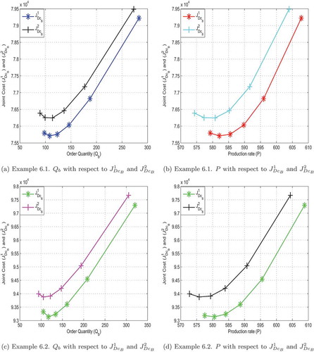
For manufacturer:A_V= 4000,$\begin{array}{rl}& H_v=10,a_1=35\times {10}^3,a_2=0.1,b_1={10}^{-4},\\ & b_2={10}^{-4},c_2={10}^{-6},\alpha =0.1,R=75,w=24,I_c=12,\\ & \gamma =1.2,w_r=80,v_r=8,w_p=100,v_p=10,E_c=20,\\ & \eta =3\times {10}^{-4},T=30,V=4.\end{array}$ Table 2 shows the optimal values of the decision variables. The graphic representations in Figure 2a and Figure 2b shows how the effect of the order quantity $Q_b$ and the rate of production P affects the joint total cost ($J_{D{c}_B}^1$ and $J_{D{c}_B}^2$) respectively.

Example 6.2 Let us consider the following numerical data to illustrate the above model.

Table 2. Optimal values of example 6.1 for case 1 and case 2 (scenario 1)

			Case 1					Case 2
n	$Q_b$	k	${\pi }_x$	P	$J_{D{c}_B}^1$	$Q_b$	k	${\pi }_x$	P	$J_{D{c}_B}^2$
	(units/year)				($/year)	(units/year)				($/year)
1	283.18	0.9844	87.2651	607.78	79,220.12	273.00	1.0108	86.8243	603.94	79,485.03
2	187.31	1.3031	83.1128	595.98	76,817.88	176.93	1.351	82.6636	591.64	77,176.95
3	146.39	1.5185	81.3405	589.78	76,035.40	136.50	1.5836	80.9122	585.23	76,464.59
4	123.23	1.6824	80.3373	585.50	75,757.37	113.87	1.7615	79.9322	580.81	76,245.90
5	108.29	1.8134	79.6903	582.12	75,711.25	99.41	1.9043	79.3058	577.32	76,253.45
6	97.87	1.9212	79.2393	579.24	75,794.19	89.40	2.0219	78.8721	574.32	76,386.84

Figure 2. Scenario: 1. The effects of order quantity and production rate on the combined total cost of case 1 and case 2

For retailer:$\begin{array}{rl}& D=500,{\mathrm{\Delta }}_1=120,{\mathrm{\Delta }}_2=90,A_b=250,H_b\\ & =30,\nu =0.01,\sigma =11,{\tau }_0=0.95,{\pi }_0=170.\end{array}$

For manufacturer:$\begin{array}{rl}& A_v=4000,H_v=10,a_1=35\times {10}^3,a_2=0.1,b_1={10}^{-4},\\ & b_2={10}^{-4},c_2={10}^{-6},\alpha =0.1,R=75,\end{array}$$\begin{array}{rl}& w=24,I_c=12,\gamma =1.2,w_r=80,v_r=8,w_p\\ & =100,v_p=10,E_c=20,\eta =3\times {10}^{-4},T=30,V=4.\end{array}$Table 3 shows the optimal values of the decision variables. The graphic representations in Figure 2c and Figure 2d shows how the effect of the order quantity $Q_b$ and the rate of production P affects the joint total cost ($J_{D{c}_B}^1$ and $J_{D{c}_B}^2$) respectively. Energy usage and carbon emission is determined using the optimal values, which are listed in Table 4.

Table 3. Optimal values of example 6.2 for case 1 and case 2 (scenario 1)

			Case 1					Case 2
n	$Q_b$	k	${\pi }_x$	P	$J_{D{c}_B}^1(.)$	$Q_b$	k	${\pi }_x$	P	$J_{D{c}_B}^2(.)$
	(units/year)				($/year)	(units/year)				($/year)
1	320.37	1.0372	94.7576	608.81	97,295.23	305.53	1.0745	94.3056	604.37	97,665.83
2	208.35	1.3985	91.3459	595.50	94,543.60	193.80	1.4649	90.9027	590.76	95,042.88
3	160.81	1.6449	89.8978	588.70	93,606.33	147.28	1.7343	89.4859	583.93	94,199.66
4	134.08	1.8336	89.0839	584.11	93,239.65	121.53	1.9419	88.7014	579.36	93,911.57
5	116.98	1.9851	88.5629	580.55	93,138.13	105.22	2.1089	88.2049	575.80	93,880.75
6	105.15	2.1097	88.2027	577.53	93,185.91	94.04	2.2466	87.8643	572.76	93,994.98

Table 4. Scenario 1. Specific energy usage and carbon emission

Example	Case	w	$w_R$	$S_{E_c}$	$GH{G}_E$
6.1	1	5921.28	5668.42	4001.04	1275.13
	2	5908.19	5655.86	4041.96	1072.72
6.2	1	5905.51	5653.29	5021.52	1728.44
	2	5858.00	5607.68	5081.59	1554.74

7 Scenario 2. Integrated methodology with reducing a lost sales

In many cases, the back-order system may not fully help the retailer, and may sometimes lose sales, so some authors have done their part to reduce lost sales in some manner (see, for instance, (Ouyang and Chang 2001), Hwang et al. (2013) and ElHafsi et al. (2021)).

In this section, the retailer doesn’t offer any price discount to the customers instead that retailer made an investment for reducing the lost sale, for convenience $1-\tau =\rho .$ The investment $\mathcal{I}(\rho )$ is a logarithmic function for reducing the lost sale. i.e.,

$\mathcal{I}(\rho )=Nln(\frac{{\rho }_0}{\rho }),\mathrm{f}\mathrm{o}\mathrm{r}0<\rho \le {\rho }_0,$

where $N=1/\omega$. The cost function of the buyer,

$\begin{array}{rl}& C_{BL}(Q_b,k,\rho ,n)=A_b\frac{D}{Q_b}\\ & +H_b\left[\frac{Q_b}{2}+k\sigma \sqrt{\nu +\frac{Q_b}{P}}\right.\\ & \left.+\frac{\sigma }{2}\sqrt{\nu +\frac{Q_b}{P}}\rho (\sqrt{1+k^2}-k)\right]\\ & +\frac{D}{2Q_b}\sigma \sqrt{\nu +\frac{Q_b}{P}}\end{array}$

(28) $\begin{array}{rl}& \times (\sqrt{1+k^2}-k)\left(\pi +{\pi }_0\rho \right)\\ & +\xi Nln\left(\frac{{\rho }_0}{\rho }\right)+\frac{nD}{Q_b}\left[T+\frac{Q_{b}V}{n}\right].\end{array}$(28)

The integrated cost function is developed by adding cost function of retailer (28) and manufacturer (10), we obtain

$J_{c_L}(Q_b,k,\rho ,P,n)=C_{BL}(Q_b,k,\rho ,n)+C_V(Q_b,P,n)$

$\begin{array}{rl}& J_{c_L}(Q_b,k,\rho ,P,n)=A_b\frac{D}{Q_b}\\ & +H_b\left[\begin{array}{c}\frac{Q_b}{2}+k\sigma \sqrt{\nu +\frac{Q_b}{P}}+\frac{\sigma }{2}\\ \sqrt{\frac{Q_b}{P}+\nu }\rho (\sqrt{1+k^2}-k)\end{array}\right]\\ & +\frac{D}{2Q_b}\sigma \sqrt{\nu +\frac{Q_b}{P}}(\sqrt{1+k^2}-k)\end{array}$

$\begin{array}{rl}& \times \left(\pi +{\pi }_0\rho \right)+\frac{nD}{Q_b}\left[T+\frac{Q_{b}V}{n}\right]+\xi Nln\left(\frac{{\rho }_0}{\rho }\right)\\ & +A_v\frac{D}{n{Q}_b}+H_v\frac{Q_b}{2}\left[n\left(1-\frac{D}{P}\right)-1+\frac{2D}{P}\right]\end{array}$

(29) $\begin{array}{rl}& +R\frac{D}{n{Q}_b}\alpha f_p\frac{{(n{Q}_b)}^2}{2P}+I_{c}D+D\left(\frac{a_1}{P}+a_{2}P\right)\\ & +W_{c}D+w\frac{D}{P}+w_R\frac{\alpha f_p\frac{{(n{Q}_b)}^2}{2P}D}{\gamma nP{Q}_b}+\eta E_{c}n{Q}_{b}D\end{array}$(29)

subject to

$0<\rho \le {\rho }_0,$

$Q_b>0,$

$n\ge 1,apositiveinteger.$

7.1 Case 1. While the quality function $f_p$ is linear in the production rate

By substituting $\frac{1}{f_p}=\frac{1}{b_{1}P}$, the integrated cost function (29) becomes

$J_{c_L}^1(Q_b,k,\rho ,P,n)=A_b\frac{D}{Q_b}+H_b\left[\frac{Q_b}{2}+k\sigma \sqrt{\nu +\frac{Q_b}{P}}+\frac{\sigma }{2}\sqrt{\nu +\frac{Q_b}{P}}\rho (\sqrt{1+k^2}-k)\right]+\frac{D}{2Q_b}\sigma \sqrt{\nu +\frac{Q_b}{P}}(\sqrt{1+k^2}-k)$

$\begin{array}{rl}& \times \left(\pi +{\pi }_0\rho \right)+\frac{nD}{Q_b}\left[T+\frac{Q_{b}V}{n}\right]\\ & +\xi Nln\left(\frac{{\rho }_0}{\rho }\right)+A_v\frac{D}{n{Q}_b}\\ & +H_v\frac{Q_b}{2}\left[n\left(1-\frac{D}{P}\right)-1+\frac{2D}{P}\right]\end{array}$

(30) $\begin{array}{rl}& +R\frac{D}{n{Q}_b}\alpha b_{1}P\frac{{(n{Q}_b)}^2}{2P}+I_{c}D+D\left(\frac{a_1}{P}+a_{2}P\right)\\ & +W_{c}D+w\frac{D}{P}+w_R\frac{\alpha b_{1}P\frac{{(n{Q}_b)}^2}{2P}D}{\gamma nP{Q}_b}+\eta E_{c}n{Q}_{b}D\end{array}$(30)

subject to

$0<\rho \le {\rho }_0,$

$Q_b>0,$

$n\ge 1,apositiveinteger.$

The fuzzified cost function of this case is given in Appendix F.

Defuzzification

Inorder to defuzzify the cost function, we substitute $\tilde{D}=\left(D+\frac{1}{4}({\mathrm{\Delta }}_2-{\mathrm{\Delta }}_1)\right)$, then (46) turns into the following equation

$J_{D{c}_L}^1=A_b\frac{\left(D+\frac{1}{4}({\mathrm{\Delta }}_2-{\mathrm{\Delta }}_1)\right)}{Q_b}+H_b\left[\frac{Q_b}{2}+k\sigma \sqrt{\nu +\frac{Q_b}{P}}+\frac{\sigma }{2}\sqrt{\nu +\frac{Q_b}{P}}\rho (\sqrt{1+k^2}-k)\right]+\frac{\left(D+\frac{1}{4}({\mathrm{\Delta }}_2-{\mathrm{\Delta }}_1)\right)}{2Q_b}$

$\times \sigma \sqrt{\nu +\frac{Q_b}{P}}(\sqrt{1+k^2}-k)\left(\pi +{\pi }_0\rho \right)+\frac{n\left(D+\frac{1}{4}({\mathrm{\Delta }}_2-{\mathrm{\Delta }}_1)\right)}{Q_b}\left[T+\frac{Q_{b}V}{n}\right]+\xi Nln\left(\frac{{\rho }_0}{\rho }\right)+\frac{A_v}{n{Q}_b}$

$\times \left(D+\frac{1}{4}({\mathrm{\Delta }}_2-{\mathrm{\Delta }}_1)\right)+H_v\frac{Q_b}{2}\left[n\left(1-\frac{\left(D+\frac{1}{4}({\mathrm{\Delta }}_2-{\mathrm{\Delta }}_1)\right)}{P}\right)-1+\frac{2\left(D+\frac{1}{4}({\mathrm{\Delta }}_2-{\mathrm{\Delta }}_1)\right)}{P}\right]$

$+R\frac{\left(D+\frac{1}{4}({\mathrm{\Delta }}_2-{\mathrm{\Delta }}_1)\right)}{n{Q}_b}\alpha b_{1}P\frac{{(n{Q}_b)}^2}{2P}+I_c\left(D+\frac{1}{4}({\mathrm{\Delta }}_2-{\mathrm{\Delta }}_1)\right)+\left(D+\frac{1}{4}({\mathrm{\Delta }}_2-{\mathrm{\Delta }}_1)\right)\left(\frac{a_1}{P}+a_{2}P\right)$

$+W_c\left(D+\frac{1}{4}({\mathrm{\Delta }}_2-{\mathrm{\Delta }}_1)\right)+w\frac{\left(D+\frac{1}{4}({\mathrm{\Delta }}_2-{\mathrm{\Delta }}_1)\right)}{P}+w_R\frac{\alpha b_{1}P\frac{{(n{Q}_b)}^2}{2P}\left(D+\frac{1}{4}({\mathrm{\Delta }}_2-{\mathrm{\Delta }}_1)\right)}{\gamma nP{Q}_b}$

(31) $+\eta E_{c}n{Q}_b\left(D+\frac{1}{4}({\mathrm{\Delta }}_2-{\mathrm{\Delta }}_1)\right)$(31)

subject to $0<\rho \le {\rho }_0,Q_b>0,n\ge 1,apositiveinteger.$

Solution procedure

In order to obtain the optimal values of the decision variables, we take first order partial derivative of (31) with respect to the $Q_b,k,\rho$ and P, by ignoring the constraints and equating to zero.

$\frac{\mathrm{\partial }{J}_{D{c}_L}^1}{\mathrm{\partial }{Q}_b}=H_b\left[\frac{1}{2}+\frac{k\sigma }{2P\sqrt{\nu +\frac{Q_b}{P}}}+\frac{\rho \sigma }{4P\sqrt{\nu +\frac{Q_b}{P}}}(\sqrt{1+k^2}-k)\right]+\left(D+\frac{1}{4}({\mathrm{\Delta }}_2-{\mathrm{\Delta }}_1)\right)\left[-\frac{A_b}{Q_b^2}-\frac{A_v}{n{Q}_b^2}\right.$

$-\frac{\sigma }{2Q_b^2}(\sqrt{1+k^2}-k)\sqrt{\nu +\frac{Q_b}{P}}[\pi +{\pi }_0\rho ]+\frac{\sigma }{4P{Q}_b\sqrt{\nu +\frac{Q_b}{P}}}(\sqrt{1+k^2}-k)[\pi +{\pi }_0\rho ]+\frac{V}{Q_b}$

$\left.-\frac{n}{Q_b^2}\left(T+\frac{Q_{b}V}{n}\right)+\frac{R\alpha n{b}_1}{2}+E_c\eta n+\frac{\alpha b_{1}n(w_r+P{v}_r\gamma )}{2P\gamma }\right]$

(32) $+\frac{H_v}{2}\left[n\left(1-\frac{\left(D+\frac{1}{4}({\mathrm{\Delta }}_2-{\mathrm{\Delta }}_1)\right)}{P}\right)-1+\text{break}\frac{2\left(D+\frac{1}{4}({\mathrm{\Delta }}_2-{\mathrm{\Delta }}_1)\right)}{P}\right]$(32)

$\frac{\mathrm{\partial }{J}_{D{c}_L}^1}{\mathrm{\partial }k}=H_b\left[\sigma \sqrt{\nu +\frac{Q_b}{P}}+\frac{\rho \sigma \sqrt{\nu +\frac{Q_b}{P}}}{2}\left(\frac{k}{\sqrt{1+k^2}}-1\right)\right]+\frac{\left(D+\frac{1}{4}({\mathrm{\Delta }}_2-{\mathrm{\Delta }}_1)\right)}{2Q_b}$

(33) $\times \left[\sigma \sqrt{\nu +\frac{Q_b}{P}}\left(\frac{k}{\sqrt{1+k^2}}-1\right)\left(\pi +{\pi }_0\rho \right)\right]$(33)

(34) $\frac{\mathrm{\partial }{J}_{D{c}_L}^1}{\mathrm{\partial }\rho }=-\frac{N\xi }{\rho }+\frac{H_b}{2}\sigma \sqrt{\nu +\frac{Q_b}{P}}(\sqrt{1+k^2}-k)+\frac{\left(D+\frac{1}{4}({\mathrm{\Delta }}_2-{\mathrm{\Delta }}_1)\right)}{2Q_b}{\pi }_0\sigma \sqrt{\nu +\frac{Q_b}{P}}(\sqrt{1+k^2}-k)$(34)

$\frac{\mathrm{\partial }{J}_{D{c}_L}^1}{\mathrm{\partial }P}=-H_b\left[\frac{Q_{b}k\sigma }{2P^2\sqrt{\nu +\frac{Q_b}{P}}}+\frac{\rho Q_b\sigma }{4P^2\sqrt{\nu +\frac{Q_b}{P}}}(\sqrt{1+k^2}-k)\right]+\left(D+\frac{1}{4}({\mathrm{\Delta }}_2-{\mathrm{\Delta }}_1)\right)\left[a_2-\frac{(w_p+P{v}_p)}{P^2}\right.$

(35) $\begin{array}{rl}& \left.\begin{array}{c}+\frac{v_p}{P}-\frac{a_1}{P^2}-H_v\frac{Q_b}{2}\left[\frac{2}{P^2}-\frac{n}{P^2}\right]-\frac{\sigma (\sqrt{1+k^2}-k)}{4P^2\sqrt{\nu +\frac{Q_b}{P}}}(\pi +\\ {\pi }_0\rho )+\frac{Q_b{v}_r\alpha b_{1}n}{2P}-\frac{Q_b\alpha b_{1}n(w_r+P{v}_r\gamma )}{2P^2\gamma }\end{array}\right]\\ & \end{array}$(35)

To achieve the global minimum of the entire supply chain model, the second-order partial derivative of $J_{D{c}_L}^1$ is taken with respect to $Q_b$ and P.

$\frac{{\mathrm{\partial }}^2{J}_{D{c}_L}^1}{\mathrm{\partial }{Q}_b^2}=\left(D+\frac{1}{4}({\mathrm{\Delta }}_2-{\mathrm{\Delta }}_1)\right)\left[\frac{2A_b}{Q_b^3}+\text{break}\frac{2A_v}{n{Q}_b^3}-\frac{2V}{Q_b^2}+\frac{2n}{Q_b^3}\left(T+\frac{Q_{b}V}{n}\right)-\frac{\sigma \sqrt{\nu +\frac{Q_b}{P}}(k-\sqrt{k^2+1})(\pi +{\pi }_0\rho )}{Q_b^3}\right.$

$\left.+\left[\frac{1}{2P{Q}_b^2\sqrt{\nu +\frac{Q_b}{P}}}+\frac{1}{8P^2{Q}_b{\left(\nu +\frac{Q_b}{P}\right)}^{\frac{3}{2}}}\right]\sigma (k-\sqrt{k^2+1})(\pi +{\pi }_0\rho )\hspace{0.17em}\right]-\frac{H_b}{{\left(\nu +\frac{Q_b}{P}\right)}^{\frac{3}{2}}}$

$\times \left[\frac{k\sigma }{4P^2}-\frac{\rho \sigma (k-\sqrt{k^2+1})}{8P^2}\right]>0$

$\begin{array}{rl}& \frac{{\mathrm{\partial }}^2{J}_{D{c}_L}^1}{\mathrm{\partial }{P}^2}=\frac{2\left(D+\frac{1}{4}({\mathrm{\Delta }}_2-{\mathrm{\Delta }}_1)\right)(w_p+P{v}_p)}{P^3}\\ & -H_b\left[\frac{Q_b^{2}k\sigma }{4P^4{\left(\nu +\frac{Q_b}{P}\right)}^{\frac{3}{2}}}-\frac{Q_{b}k\sigma }{P^3\sqrt{\nu +\frac{Q_b}{P}}}\right.\\ & +\left(\frac{Q_b\rho \sigma }{2P^3\sqrt{\nu +\frac{Q_b}{P}}}-\frac{Q_b^2\rho \sigma }{8P^4{\left(\nu +\frac{Q_b}{P}\right)}^{\frac{3}{2}}}\right)\end{array}$

$\begin{array}{rl}& \times \left.(k-\sqrt{k^2+1})\right]+\left(D+\frac{1}{4}({\mathrm{\Delta }}_2-{\mathrm{\Delta }}_1)\right)\\ & \left[\frac{2a_1}{P^3}-\frac{2v_p}{P^2}+H_v\frac{Q_b}{2}\left(\frac{4}{P^3}-\frac{2n}{P^3}\right)-\frac{Q_b{v}_r\alpha b_{1}n}{P^2}\right.\end{array}$

$\begin{array}{rl}& -\frac{\sigma (k-\sqrt{k^2+1})(\pi +{\pi }_0\rho )}{2P^3\sqrt{\nu +\frac{Q_b}{P}}}\\ & +\frac{\sigma Q_b}{8P^4{\left(\nu +\frac{Q_b}{P}\right)}^{\frac{3}{2}}}(\pi +{\pi }_0\rho )(k-\sqrt{k^2+1})\\ & \left.+\frac{Q_b\alpha b_{1}n(w_r+P{v}_r\gamma )}{P^3\gamma }\right]>0\end{array}$

where, $J_{D{c}_L}^1=J_{D{c}_L}^1(Q_b,k,\rho ,P,n).$

Proposition 7.1 For fixed values of $Q_b$, ρ, P and n, the objective function $J_{D{c}_L}^1(Q_b,k,\rho ,P,n)$ (31) is convex in k, there exists a unique value for the safety factor $k=k^{\ast }(Q_b,\rho ,P,n)$ that minimizes the cost function $J_{D{c}_L}^1(Q_b,k,\rho ,P,n)$. For fixed values of $Q_b$, k, P and n, the objective function $J_{D{c}_L}^1(Q_b,k,\rho ,P,n)$ (31) is convex in ρ, there exists a unique value for the lost sale $\rho ={\rho }^{\ast }(Q_b,k,P,n)$ that minimizes the cost function $J_{D{c}_L}^1(Q_b,k,\rho ,P,n)$.

Proof. Appendix C.

Proposition 7.2 For fixed values of $Q_b$, k, ${\pi }_x$ and P, $J_{D{c}_L}^1(Q_b,k,\rho ,P,n)$ (31) is a convex function on n.

Proof. Appendix B.

7.2 Case 2. While the quality function $f_p$ is quadratic in the production rate

By substituting $\frac{1}{f_p}=\frac{1}{b_{2}P+c_2{P}^2}$, the integrated cost function (12) becomes

$\begin{array}{rl}& J_{c_L}^2(Q_b,k,\rho ,P,n)=A_b\frac{D}{Q_b}\\ & +H_b\left[\frac{Q_b}{2}+k\sigma \sqrt{\nu +\frac{Q_b}{P}}\right.\\ & \left.+\frac{\sigma }{2}\sqrt{\nu +\frac{Q_b}{P}}\rho (\sqrt{1+k^2}-k)\right]\\ & +\frac{D}{2Q_b}\sigma \sqrt{\nu +\frac{Q_b}{P}}(\sqrt{1+k^2}-k)\end{array}$

$\begin{array}{rl}& \times \left(\pi +{\pi }_0\rho \right)+\frac{nD}{Q_b}\left[T+\frac{Q_{b}V}{n}\right]+\xi Nln\left(\frac{{\rho }_0}{\rho }\right)\\ & +A_v\frac{D}{n{Q}_b}+H_v\frac{Q_b}{2}\left[n\left(1-\frac{D}{P}\right)-1+\frac{2D}{P}\right]\end{array}$

$\begin{array}{rl}& +R\frac{D}{n{Q}_b}\alpha (b_{2}P+c_2{P}^2)\frac{{(n{Q}_b)}^2}{2P}\\ & +I_{c}D+D\left(\frac{a_1}{P}+a_{2}P\right)+W_{c}D+w\frac{D}{P}\\ & +w_R\frac{\alpha (b_{2}P+c_2{P}^2)\frac{{(n{Q}_b)}^2}{2P}D}{\gamma nP{Q}_b}\end{array}$

(36) $+\eta E_{c}n{Q}_{b}D$(36)

subject to

$0<\rho \le {\rho }_0,$

$Q_b>0,$

$n\ge 1,apositiveinteger.$

The fuzzified cost function of this case is given in Appendix F.

Defuzzification

We follow the same procedure for the defuzzification process, by substituting $\tilde{D}=\left(D+\frac{1}{4}({\mathrm{\Delta }}_2-{\mathrm{\Delta }}_1)\right)$ on (47), we obtain the defuzzified cost as

$J_{D{c}_L}^2=A_b\frac{\left(D+\frac{1}{4}({\mathrm{\Delta }}_2-{\mathrm{\Delta }}_1)\right)}{Q_b}+H_b\left[\frac{Q_b}{2}+k\sigma \sqrt{\nu +\frac{Q_b}{P}}+\frac{\sigma }{2}\sqrt{\nu +\frac{Q_b}{P}}\rho (\sqrt{1+k^2}-k)\right]+\frac{\left(D+\frac{1}{4}({\mathrm{\Delta }}_2-{\mathrm{\Delta }}_1)\right)}{2Q_b}$

$\times \sigma \sqrt{\nu +\frac{Q_b}{P}}(\sqrt{1+k^2}-k)\left(\pi +{\pi }_0\rho \right)+\frac{n\left(D+\frac{1}{4}({\mathrm{\Delta }}_2-{\mathrm{\Delta }}_1)\right)}{Q_b}\left[T+\frac{Q_{b}V}{n}\right]+\xi Nln\left(\frac{{\rho }_0}{\rho }\right)$

$+A_v\frac{\left(D+\frac{1}{4}({\mathrm{\Delta }}_2-{\mathrm{\Delta }}_1)\right)}{n{Q}_b}+H_v\frac{Q_b}{2}\left[\begin{array}{c}n\left(1-\frac{\left(D+\frac{1}{4}({\mathrm{\Delta }}_2-{\mathrm{\Delta }}_1)\right)}{P}\right)\\ -1+\frac{2\left(D+\frac{1}{4}({\mathrm{\Delta }}_2-{\mathrm{\Delta }}_1)\right)}{P}\end{array}\right]$

$+R\frac{\left(D+\frac{1}{4}({\mathrm{\Delta }}_2-{\mathrm{\Delta }}_1)\right)}{n{Q}_b}\alpha (b_{2}P+c_2{P}^2)\frac{{(n{Q}_b)}^2}{2P}+I_c\left(D+\frac{1}{4}({\mathrm{\Delta }}_2-{\mathrm{\Delta }}_1)\right)+\left(D+\frac{1}{4}({\mathrm{\Delta }}_2-{\mathrm{\Delta }}_1)\right)$

$\times \left(\frac{a_1}{P}+a_{2}P\right)+W_c\left(D+\frac{1}{4}({\mathrm{\Delta }}_2-{\mathrm{\Delta }}_1)\right)+w\frac{\left(D+\frac{1}{4}({\mathrm{\Delta }}_2-{\mathrm{\Delta }}_1)\right)}{P}+w_R\frac{\alpha (b_{2}P+c_2{P}^2)\frac{{(n{Q}_b)}^2}{2P}}{\gamma nP{Q}_b}$

(37) $\times \left(D+\frac{1}{4}({\mathrm{\Delta }}_2-{\mathrm{\Delta }}_1)\right)+\eta E_{c}n{Q}_b\left(D+\frac{1}{4}({\mathrm{\Delta }}_2-{\mathrm{\Delta }}_1)\right)$(37)

subject to $0<\rho \le {\rho }_0,Q_b>0,n\ge 1,apositiveinteger.$

Solution procedure

To obtain the optimal values of the decision variables, we take first order partial derivative of (37) with respect to the $Q_b,k,\rho$ and P, by ignoring the constraints and equating to zero.

$\frac{\mathrm{\partial }{J}_{D{c}_L}^2}{\mathrm{\partial }{Q}_b}=-\frac{A_b\left(D+\frac{1}{4}({\mathrm{\Delta }}_2-{\mathrm{\Delta }}_1)\right)}{Q_b^2}+H_b\left[\frac{1}{2}+\frac{k\sigma }{2P\sqrt{\nu +\frac{Q_b}{P}}}+\frac{\rho \sigma }{4P\sqrt{\nu +\frac{Q_b}{P}}}(\sqrt{1+k^2}-k)\right]-\frac{\left(D+\frac{1}{4}({\mathrm{\Delta }}_2-{\mathrm{\Delta }}_1)\right)}{2Q_b^2}$

$\begin{array}{rl}& \times \sigma (\sqrt{1+k^2}-k)\sqrt{\nu +\frac{Q_b}{P}}[\pi +{\pi }_0\rho ]+\\ & \frac{\left(D+\frac{1}{4}({\mathrm{\Delta }}_2-{\mathrm{\Delta }}_1)\right)\sigma }{4P{Q}_b\sqrt{\nu +\frac{Q_b}{P}}}(\sqrt{1+k^2}-k)[\pi +{\pi }_0\rho ]-\frac{A_v}{n{Q}_b^2}\end{array}$

$\times \left(D+\frac{1}{4}({\mathrm{\Delta }}_2-{\mathrm{\Delta }}_1)\right)+\frac{H_v}{2}\left[n\left(1-\frac{\left(D+\frac{1}{4}({\mathrm{\Delta }}_2-{\mathrm{\Delta }}_1)\right)}{P}\right)-1+\frac{2\left(D+\frac{1}{4}({\mathrm{\Delta }}_2-{\mathrm{\Delta }}_1)\right)}{P}\right]$

$+\frac{V\left(D+\frac{1}{4}({\mathrm{\Delta }}_2-{\mathrm{\Delta }}_1)\right)}{Q_b}-\frac{n\left(D+\frac{1}{4}({\mathrm{\Delta }}_2-{\mathrm{\Delta }}_1)\right)}{Q_b^2}\left(T+\frac{Q_{b}V}{n}\right)+\frac{\left(D+\frac{1}{4}({\mathrm{\Delta }}_2-{\mathrm{\Delta }}_1)\right)R\alpha n(c_2{P}^2+b_{2}P)}{2P}$

(38) $\begin{array}{rl}& +E_c\eta n\left(D+\frac{1}{4}({\mathrm{\Delta }}_2-{\mathrm{\Delta }}_1)\right)+\frac{\left(D+\frac{1}{4}({\mathrm{\Delta }}_2-{\mathrm{\Delta }}_1)\right)}{2P^2\gamma }\\ & \alpha n(w_r+P{v}_r\gamma )(c_2{P}^2+b_{2}P)\end{array}$(38)

$\frac{\mathrm{\partial }{J}_{D{c}_L}^2}{\mathrm{\partial }k}=H_b\left[\sigma \sqrt{\nu +\frac{Q_b}{P}}+\frac{\rho \sigma \sqrt{\nu +\frac{Q_b}{P}}}{2}\left(\frac{k}{\sqrt{1+k^2}}-1\right)\right]+\frac{\left(D+\frac{1}{4}({\mathrm{\Delta }}_2-{\mathrm{\Delta }}_1)\right)}{2Q_b}$

(39) $\times \left[\sigma \sqrt{\nu +\frac{Q_b}{P}}\left(\frac{k}{\sqrt{1+k^2}}-1\right)(\pi +{\pi }_0)\rho \right]$(39)

(40) $\frac{\mathrm{\partial }{J}_{D{c}_L}^2}{\mathrm{\partial }\rho }=-\frac{N\xi }{\rho }+\frac{H_b}{2}\sigma \sqrt{\nu +\frac{Q_b}{P}}(\sqrt{1+k^2}-k)+\frac{\left(D+\frac{1}{4}({\mathrm{\Delta }}_2-{\mathrm{\Delta }}_1)\right)}{2Q_b}{\pi }_0\sigma \sqrt{\nu +\frac{Q_b}{P}}(\sqrt{1+k^2}-k)$(40)

$\frac{\mathrm{\partial }{J}_{D{c}_L}^2}{\mathrm{\partial }P}=a_2\left(D+\frac{1}{4}({\mathrm{\Delta }}_2-{\mathrm{\Delta }}_1)\right)-H_b\left[\frac{Q_{b}k\sigma }{2P^2\sqrt{\nu +\frac{Q_b}{P}}}+\frac{\rho Q_b\sigma }{4P^2\sqrt{\nu +\frac{Q_b}{P}}}(\sqrt{1+k^2}-k)\right]-\frac{\left(D+\frac{1}{4}({\mathrm{\Delta }}_2-{\mathrm{\Delta }}_1)\right)}{P^2}$

$\begin{array}{rl}& \times (w_p+P{v}_p)+\frac{v_p\left(D+\frac{1}{4}({\mathrm{\Delta }}_2-{\mathrm{\Delta }}_1)\right)}{P}\\ & -\frac{a_1\left(D+\frac{1}{4}({\mathrm{\Delta }}_2-{\mathrm{\Delta }}_1)\right)}{P^2}-H_v\frac{Q_b}{2}\left[\frac{2\left(D+\frac{1}{4}({\mathrm{\Delta }}_2-{\mathrm{\Delta }}_1)\right)}{P^2}\right.\end{array}$

$\left.-\frac{n\left(D+\frac{1}{4}({\mathrm{\Delta }}_2-{\mathrm{\Delta }}_1)\right)}{P^2}\right]-\frac{\left(D+\frac{1}{4}({\mathrm{\Delta }}_2-{\mathrm{\Delta }}_1)\right)\sigma (\sqrt{1+k^2}-k)}{4P^2\sqrt{\nu +\frac{Q_b}{P}}}(\pi +{\pi }_0\rho )+\frac{Q_b\left(D+\frac{1}{4}({\mathrm{\Delta }}_2-{\mathrm{\Delta }}_1)\right)}{2P}$

(41) $\begin{array}{rl}& \times R\alpha n(b_2+2P{c}_2)-\frac{Q_b\left(D+\frac{1}{4}({\mathrm{\Delta }}_2-{\mathrm{\Delta }}_1)\right)}{2P^2}R\alpha n(c_2{P}^2+b_{2}P)\\ & +\frac{\left(D+\frac{1}{4}({\mathrm{\Delta }}_2-{\mathrm{\Delta }}_1)\right)Q_b}{2P^2}{v}_r\alpha n(c_2{P}^2+b_{2}P)\\ & -\frac{\left(D+\frac{1}{4}({\mathrm{\Delta }}_2-{\mathrm{\Delta }}_1)\right)Q_b}{2P^2\gamma }\alpha n(w_r+P{v}_r\gamma )(b_2{P}^2+2P{c}_2)\\ & -\frac{\left(D+\frac{1}{4}({\mathrm{\Delta }}_2-{\mathrm{\Delta }}_1)\right)Q_b}{P^3\gamma }\alpha n(w_r+P{v}_r\gamma )(c_2{P}^2+b_{2}P)\end{array}$(41)

To achieve the global minimum of the entire supply chain model, the second-order partial derivative of $J_{D{c}_L}^1$ is taken with respect to $Q_b$ and P.

$\begin{array}{rl}& \frac{{\mathrm{\partial }}^2{J}_{D{c}_L}^2}{\mathrm{\partial }{Q}_b^2}=\left(D+\frac{1}{4}({\mathrm{\Delta }}_2-{\mathrm{\Delta }}_1)\right)\\ & \left[\frac{2A_b}{Q_b^3}+\frac{2A_v}{n{Q}_b^3}-\frac{2V}{Q_b^2}+\frac{2n}{Q_b^3}\left(T+\frac{Q_{b}V}{n}\right)\right.\\ & -\frac{\sigma \sqrt{\nu +\frac{Q_b}{P}}(k-\sqrt{k^2+1})(\pi +{\pi }_0\rho )}{Q_b^3}\end{array}$

$\left.+\left[\begin{array}{c}\frac{1}{2P{Q}_b^2\sqrt{\nu +\frac{Q_b}{P}}}\\ +\frac{1}{8P^2{Q}_b{\left(\nu +\frac{Q_b}{P}\right)}^{\frac{3}{2}}}\end{array}\right]\sigma (k-\sqrt{k^2+1})(\pi +{\pi }_0\rho )\right]-\frac{H_b}{{\left(\nu +\frac{Q_b}{P}\right)}^{\frac{3}{2}}}$

(42) $\times \left[\frac{k\sigma }{4P^2}-\frac{\rho \sigma (k-\sqrt{k^2+1})}{8P^2}\right]>0$(42)

$\begin{array}{rl}& \frac{{\mathrm{\partial }}^2{J}_{D{c}_L}^2}{\mathrm{\partial }{P}^2}=\frac{2\left(D+\frac{1}{4}({\mathrm{\Delta }}_2-{\mathrm{\Delta }}_1)\right)(w_p+P{v}_p)}{P^3}\\ & -H_b\left[\frac{Q_b^{2}k\sigma }{4P^4{\left(\nu +\frac{Q_b}{P}\right)}^{\frac{3}{2}}}-\frac{Q_{b}k\sigma }{P^3\sqrt{\nu +\frac{Q_b}{P}}}\right.\\ & +\left(\frac{Q_b\rho \sigma }{2P^3\sqrt{\nu +\frac{Q_b}{P}}}-\frac{Q_b^2\rho \sigma }{8P^4{\left(\nu +\frac{Q_b}{P}\right)}^{\frac{3}{2}}}\right)\end{array}$

$\begin{array}{rl}& \times \left.(k-\sqrt{k^2+1})\right]+\left(D+\frac{1}{4}({\mathrm{\Delta }}_2-{\mathrm{\Delta }}_1)\right)\\ & \left[\frac{2a_1}{P^3}-\frac{2v_p}{P^2}+H_v\frac{Q_b}{2}\left(\frac{4}{P^3}-\frac{2n}{P^3}\right)\right.\\ & -(k-\sqrt{k^2+1})\end{array}$

$\begin{array}{rl}& \times \left(\frac{\sigma }{2P^3\sqrt{\nu +\frac{Q_b}{P}}}-\frac{Q_b\sigma }{8P^4{\left(\nu +\frac{Q_b}{P}\right)}^{\frac{3}{2}}}\right)(\pi +{\pi }_0\rho )\\ & +\frac{Q_{b}R\alpha c_{2}n}{P}+\left(v_r-R\right)\frac{Q_b\alpha n(b_2+2P{c}_2)}{P^2}\end{array}$

$\begin{array}{rl}& +\left(R-2v_r\right)\frac{Q_b\alpha n}{P^3}(c_2{P}^2+b_{2}P)\\ & +\left(\frac{3(c_2{P}^2+b_{2}P)}{P^4\gamma }-\frac{2(b_2+2P{c}_2)}{P^3\gamma }+\frac{c_2}{P^2\gamma }\right)\end{array}$

(43) $\times \left.Q_b\alpha n(w_r+P{v}_r\gamma )\right]>0$(43)

where, $J_{D{c}_L}^2=J_{D{c}_L}^2(Q_b,k,\rho ,P,n).$

Proposition 7.3 For fixed values of $Q_b$, ρ, P and n, the objective function $J_{D{c}_L}^2(Q_b,k,\rho ,P,n)$ (37) is convex in k, there exists a unique value for the safety factor $k=k^{\ast }(Q_b,\rho ,P,n)$ that minimizes the cost function $J_{D{c}_L}^2(Q_b,k,\rho ,P,n)$. For fixed values of $Q_b$, k, P and n, the objective function $J_{D{c}_L}^2(Q_b,k,\rho ,P,n)$ (37) is convex in ρ, there exists a unique value for the lost sale $\rho ={\rho }^{\ast }(Q_b,k,P,n)$ that minimizes the cost function $J_{D{c}_L}^2(Q_b,k,\rho ,P,n)$.

Proof. Appendix C.

Proposition 7.4 For fixed values of $Q_b$, k, ρ and P, $J_{D{c}_L}^2(Q_b,k,\rho ,P,n)$ (37) is a convex function on n.

Proof. Appendix D.

7.3 Algorithm

Step 1 Set $n^j=1$ where, $j=1,2$ (for cases 1, 2).

Step 2 For each $i=1,2,\dots ,m$ do the following steps.

Step 2(i) First, initialize the values for $k_1^j=0,{\rho }_1^j={\rho }_0\mathrm{a}\mathrm{n}\mathrm{d}{P}^j$.

Step 2(ii) Using the values of $k_1^j,{\rho }_1^j,\mathrm{a}\mathrm{n}\mathrm{d}{P}^j$ and compute $Q_{b1}^j$ by solving (32) and (38).

Step 2(iii) Using the values of $Q_{b1}^j,{\rho }_1^j,\mathrm{a}\mathrm{n}\mathrm{d}{P}^j$ and compute $k_2^j$ by solving (33) and (39).

Step 2(iv) Using the values of $Q_{b1}^j,k_2^j,\mathrm{a}\mathrm{n}\mathrm{d}{P}^j$ and compute ${\rho }_2^j$ by solving (34) and (40).

Step 2(v) Repeat the steps $2(i)and2(iv)$ until the values of $Q_{bi}^j$, $k_{(i+1)}^j$, ${\rho }_{(i+1)}^j$ ($i=2,3,\dots ,m$), occurs no change and denote the values as $Q_{bi}^{j\ast }$, $k_i^{j\ast }$, ${\rho }_i^{j\ast }$.

Step 2(vi) Using the values of $Q_{bi}^{j\ast },k_i^{j\ast },\mathrm{a}\mathrm{n}\mathrm{d}{\rho }_i^{j\ast }$ and compute ${\rho }^{\left\{j^{\ast }\right\}}$ solving (35) and (41).

Step 3 Compute $J_{D{c}_L}^j(Q_{bi}^{j\ast },k_i^{j\ast },{\rho }_i^{j\ast },P^{j\ast },n^{j\ast })$ using the values of $Q_{bi}^{j\ast }$, $k_i^{j\ast }$, ${\rho }_i^{j\ast }$ and $P^{j\ast }$.

Step 4 Set $n^j=n^j+1$, repeat the Steps from 2 to 3.

Step 5 $J_{D{c}_L}^j(Q_b^{j\ast },k^{j\ast },{\rho }^{j\ast },P^{j\ast },n^{j\ast })$=${min}_{i=1,2,3,\dots ,m}$

$J_{D{c}_L}^j(Q_{bi}^{j\ast },k_i^{j\ast },{\rho }_i^{j\ast },P^{j\ast },n^{j\ast })$ and we obtain

$J_{D{c}_L}^j(Q_b^{j\ast },k^{j\ast },{\rho }^{j\ast },P^{j\ast },n^{j\ast })$ as the optimal solution.

7.4 Numerical examples

Example 7.1 Let us consider the following numerical data to illustrate the above model.

For retailer: $D=400,{\mathrm{\Delta }}_1=100,{\mathrm{\Delta }}_2=70,A_b=350,H_b=34,\nu =0.01,\sigma =10,{\pi }_0=150,\pi =50,{\rho }_0=1,$ $\xi =0.1,N=125.$ For manufacturer: $\begin{array}{rl}& A_v=4000,H_v=10,a_1=35\times \\ & {10}^3,a_2=0.1,b_1={10}^{-4},b_2={10}^{-4},c_2={10}^{-6},\alpha =0.1,R=\\ & 75,w=24,I_c=12,\gamma =1.2,w_r=80,v_r=8,w_p=100,v_p=\\ & 10,E_c=20,\eta =3\times {10}^{-4},T=30,V=4.\end{array}$

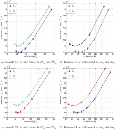
The optimal values of the decision variables are shown in Table 5 using the above data. The graphic representations in Figure 3a and Figure 3b shows how the effect of the order quantity $Q_b$ and the production rate P affects the joint total cost ($J_{D{c}_L}^1$ and $J_{D{c}_L}^2$) respectively.

Example 7.2 Let us consider the following numerical data to illustrate the above model.

For retailer: $D=500,{\mathrm{\Delta }}_1=120,{\mathrm{\Delta }}_2=90,A_b=250,H_b=30,\nu =0.01,\sigma =11,{\pi }_0=170,\pi =60,{\rho }_0=1,\xi =0.1,$ $N=140$. For manufacturer: $A_v=4000,H_v=10,a_1=35\times {10}^3,a_2=0.1,b_1={10}^{-4},b_2={10}^{-4},c_2={10}^{-6},\alpha =0.1,R=75,$ $\begin{array}{rl}& w=24,I_c=12,\gamma =1.2,w_r=80,v_r=8,w_p=100,v_p=10,\\ & E_c=20,\eta =3\times {10}^{-4},T=30,V=4.\end{array}$The optimal values of the decision variables are shown in Table 6 using the above data. The graphic representations in Figure 3c and Figure 3d shows how the effect of the order quantity $Q_b$ and the rate of production P affects the joint total cost ($J_{D{c}_L}^1$ and $J_{D{c}_L}^2$) respectively. Table 7 shows the energy usage and carbon emission determined using the optimal values.

Table 5. Optimal values of example 7.1 for case 1 and case 2 (scenario 2)

			Case 1					Case 2
n	$Q_b$	k	p	P	$J_{D{c}_L}^1$	$Q_b$	k	ρ	P	$J_{D{c}_L}^2$
	(units/year)				($/year)	(units/year)				($/year)
1	284.93	0.0796	0.02071	605.95	78,965.58	274.53	0.1146	0.0211	602.12	79,231.88
2	188.05	0.4335	0.0246	594.28	76,589.32	177.54	0.4788	0.0250	589.96	76,949.65
3	146.81	0.6271	0.0262	588.14	75,816.50	136.83	0.6820	0.0265	583.63	76,246.81
4	123.50	0.7624	0.0270	583.90	75,543.43	114.07	0.8253	0.0273	579.26	76,032.93
5	108.47	0.8656	0.0275	580.55	75,500.20	99.54	0.9352	0.0278	575.80	76,043.23
6	98.00	0.9479	0.0278	577.69	75,584.96	89.48	1.0233	0.0281	572.82	76,178.29

Table 6. Optimal values of example 7.2 for case 1 and case 2 (scenario 2)

			Case 1					Case 2
$n$	$Q_b$	k	ρ	P	$J_{D{c}_L}^1$	$Q_b$	k	$\rho$	$P$	$J_{D{c}_L}^2$
	(units/year)				($/year)	(units/year)				($/year)
1	321.30	0.4258	0.0230	607.68	97,116.84	306.32	0.4635	0.0233	603.26	97,488.14
2	208.75	0.7632	0.0255	594.43	94,378.20	194.11	0.8208	0.0258	589.71	94,878.16
3	161.02	0.9722	0.0264	587.66	93,445.77	147.44	1.0458	0.0267	582.91	94,039.69
4	134.21	1.126	0.0269	583.09	93,081.51	121.61	1.2124	0.0271	578.36	93,753.91
5	117.06	1.2465	0.0272	579.53	92,981.31	105.27	1.3436	0.0274	574.81	93,724.30
6	105.20	1.3442	0.0274	576.52	93,029.84	94.07	1.4502	0.0275	571.79	93,839.18

Table 7. Scenario 2. specific energy usage and carbon emission

Example	Case	w	$w_R$	$S_{E_c}$	$GH{G}_E$
7.1	1	5905.58	5653.35	4001.24	1277.29
	2	5892.62	5640.91	4042.12	1074.59
7.2	1	5895.38	5643.57	5021.67	1729.62
	2	5848.17	5598.24	5081.66	1555.41

Figure 3. Scenario: 2. The effects of order quantity and production rate on the combined total cost of case 1 and case 2

8 Sensitivity analysis and managerial implications

In this section, sensitivity analysis is performed for the core parameters of the proposed model. The parameters which are considered for this analysis are $E_c,w,w_r,v_r,w_p,V_p$ and R. The sensitivity results are provided in Table 8. Figure 4 (4a, 4b, 4 c, 4d, 4e, 4 f, 4 g) and Figure 5 (5a, 5b, 5 c, 5d, 5e, 5 f, 5 g) illustrates sensitivity graph of case 1 and case 2 in both scenarios respectively. $w$ is found to be more sensitive compared with other parameters. $V_P$ and $E_c$ are found to be slightly sensitive than $w_r,V_r,w_P$ and R.

Table 8. Sensitivity analysis

Parameters	% changes	Case 1		Case 2
		Scenario – 1	Scenario – 2	Scenario – 1	Scenario – 2
$E_c$	−50 %	75,001.9019	74,786.9880	75,564.8010	75,350.5302
	−25 %	75,357.9077	75,144.4233	75,899.5474	75,686.4918
	+25 %	76,029.0556	75,817.8940	76,507.4282	76,293.8573
	+50 %	76,334.7631	76,122.0491	76,781.8343	76,569.1913
w	−50 %	70,989.7697	70,777.5240	71,514.9989	71,300.4839
	−25 %	73,344.7917	73,132.5240	73,867.4235	73,655.4839
	+25 %	78,054.7697	77,842.5240	78,577.4235	78,365.4388
	+50 %	80,409.8169	80,197.5240	80,932.4235	80,720.4839
$w_r$	−50 %	75,699.7174	75,487.4595	76,224.6255	76,010.0236
	−25 %	75,699.7376	75,487.4918	76,222.2185	76,010.2312
	+25 %	75,699.8017	75,487.5563	76,222.6304	76,010.6714
	+50 %	75,699.8338	75,487.5885	76,222.8393	76,010.8588
$V_r$	−50 %	75,695.2975	75,483.0364	76,193.7819	75,981.7744
	−25 %	75,697.5339	75,485.2804	76,208.1145	75,997.4699
	+25 %	75,702.0245	75,489.7670	76,237.9776	76,024.7353
	+50 %	75,704.2397	75,492.1208	76,250.9367	76,039.0083
$w_P$	−50 %	75,666.0027	75,453.6618	76,188.3562	75,976.5276
	−25 %	75,683.0861	75,470.5961	76,205.3779	75,993.5089
	+25 %	75,716.6438	75,504.4456	76,239.4630	76,027.5257
	+50 %	75,733.5117	75,521.3610	76,256.4962	76,044.8792
$V_P$	−50 %	73,737.3076	73,525.0240	74,260.0250	74,047.9496
	−25 %	74,718.5197	74,506.2740	75,241.1735	75,029.2340
	+25 %	76,681.0198	76,468.7749	77,203.7623	76,992.2312
	+50 %	77,662.2901	77,450.0240	78,184.9249	77,972.9388
R	−50 %	75,657.7539	75,445.3629	75,950.1679	75,737.8528
	−25 %	75,678.7865	75,466.4683	76,087.3342	75,875.2392
	+25 %	75,720.7428	75,508.5721	76,345.9151	76,131.5419
	+50 %	75,741.5989	75,529.4869	76,465.2476	76,250.9341

Figure 4. Sensitivity analysis of $E_c,w,w_r,V_r,w_P,V_P$ and R with respect to the joint cost for Scenario – 1 and 2 (Case-1)

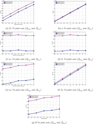
Figure 5. Sensitivity analysis of $E_c,w,w_r,V_r,w_P,V_P$ and R with respect to the joint cost for Scenario – 1 and 2 (Case-2)

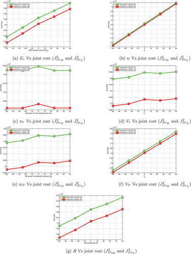
From this article, managers can explore a variety of ways to create better deals and limit the production of products without harming the environment. By looking at the high range of overall (GHG) emissions, manufacturing companies can optimise their current resources and make full use of all available resources and determine how much of each product they can afford to stay within the GHG emissions range. Higher production levels affect environmental performance, such as energy consumption and greenhouse gas emissions. When looking at the specific energy use from both scenarios, it is almost identical. Also, carbon emissions appear to be slightly higher in the second scenario than in the first scenario. Defective materials are exposed in the event of a malfunction in the engine during rapid production, so this model is capable of adapting production to suit the environment. In addition, managers can take advantage of this model to determine whether discounting the cost of goods to the customer reduces the total cost or reduces the total cost by reducing lost sales despite offering no discounts.

9 Conclusion

This article is designed to reduce the total cost in two different scenarios, including the need for energy during perfect and imperfect production, greenhouse gas emissions, and when the demand for the product is fuzzy (ambiguous) under the integrated green supply chain model. In order to relate process quality and production rate, two different cases are explored in each situation. This research aims to analyse which scenario is appropriate to obtain the minimum total cost in the fuzzy environment. The retailer’s demand is considered to be a triangular fuzzy number because the demand for the product may be ambiguous under certain circumstances. The reworking process is considered if there are any defective items produced during the production. In this regard, we have compared the single supply chain model in two scenarios, whereby investing to reduce lost sales enables supply chain partners to obtain a minimum total cost than providing discounts on backorder.

The proposed model’s extension can be implemented in several ways by treating the demand rate with different fuzzy numbers such as the trapezoidal, pentagonal and hexagonal fuzzy number. Considering multiple retailers with multiple items would be a reasonable extension of this model. If the greenhouse emissions exceed the limit, the penalty cost of expelling more gases from industries would be another beneficial extension of this model. The practical study of inspection process under controllable lead time would be another extension. Moreover, this model can be extended by recycling unwanted and used materials to create a circular economy model. Furthermore, this model can be extended by considering the carbon emission function depending on the production rate.

Acknowledgments

The work of the authors are supported by UGC - SAP (DSA - I), Department of Mathematics, The Gandhigram Rural Institute (Deemed to be University) Gandhigram, Dindigul District, Tamil Nadu, India. Pincode: 624 302.

Disclosure statement

No potential conflict of interest was reported by the author(s).

Additional information

Notes on contributors

B. Karthick

B. Karthick received his Bachelor of Science and Master of Science degrees in Mathematics in 2016 and 2018, respectively, from The Gandhigram Rural Institute (Deemed to be University), Gandhigram, Tamilnadu, India. He is currently a Full-Time PhD Research Scholar in the Department of Mathematics, The Gandhigram Rural Institute (Deemed to be University), Gandhigram, Tamilnadu, India. His current research interests include operations research, inventory control, fuzzy optimization and supply chain management.

R. Uthayakumar

R. Uthayakumar obtained his Master of Science in Mathematics in 1989 from The American College, Madurai, Tamilnadu, India. He completed his Master of Philosophy in Mathematics at Madurai Kamaraj University, Madurai, Tamilnadu, India. He is currently a Professor in the Department of Mathematics, The Gandhigram Rural Institute (Deemed to be University), Gandhigram, Tamilnadu, India. He has published about 220 articles in national and international journals. His research interests include fractal geometry, optimization techniques, inventory control, fuzzy decision making and supply chain management.

Appendix A

On taking second-order partial derivatives of (17) and (23) with respect to k and ${\pi }_x$, we get

$\frac{{\mathrm{\partial }}^2{J}_{D{c}_B}}{\mathrm{\partial }{k}^2}=\frac{H_b}{2}\sigma \sqrt{\nu +\frac{Q_b}{P}}\left(1-\frac{{\tau }_0{\pi }_x}{{\pi }_0}\right)\left[\frac{1}{\sqrt{1+k^2}}-\frac{k^2}{{(1+k^2)}^{\frac{3}{2}}}\right]+\frac{\left(D+\frac{1}{4}({\mathrm{\Delta }}_2-{\mathrm{\Delta }}_1)\right)\sigma }{2Q_b}\sqrt{\nu +\frac{Q_b}{P}}$

$\times \left[\frac{k^2}{{(1+k^2)}^{\frac{3}{2}}}-\frac{1}{\sqrt{1+k^2}}\right]\left[{\pi }_0\left(\frac{{\tau }_0{\pi }_x}{{\pi }_0}-1\right)-\frac{{\tau }_0{\pi }_x^2}{{\pi }_0}\right]>0$

$\frac{{\mathrm{\partial }}^2{J}_{D{c}_B}}{\mathrm{\partial }{\pi }_x^2}=\frac{\left(D+\frac{1}{4}({\mathrm{\Delta }}_2-{\mathrm{\Delta }}_1)\right){\tau }_0\sigma }{Q_b{\pi }_0}\sqrt{\nu +\frac{Q_b}{P}}(\sqrt{1+k^2}-k)>0$

where, $J_{D{c}_B}=J_{D{c}_B}^1(\mathrm{o}\mathrm{r})J_{D{c}_B}^2.$ This shows that $J_{D{c}_B}^1(Q_b,k,{\pi }_x,P,n)$ and $J_{D{c}_B}^2(Q_b,k,{\pi }_x,P,n)$ is convex on k and ${\pi }_x$. Hence, this completes the proof of Proposition 6.1 and 6.3.

Appendix B

If we take the first and second-order partial derivatives of (17) and (31) with respect to n, we get

$\frac{\mathrm{\partial }{J}_{Dc}^1}{\mathrm{\partial }n}=H_v\frac{Q_b}{2}\left(1-\frac{\left(D+\frac{1}{4}({\mathrm{\Delta }}_2-{\mathrm{\Delta }}_1)\right)}{P}\right)+\left(D+\frac{1}{4}({\mathrm{\Delta }}_2-{\mathrm{\Delta }}_1)\right)\left[\left(T+\frac{Q_{b}V}{n}\right)\frac{1}{Q_b}-\frac{V}{n}\right.$

$\left.-\frac{A_v}{Q_b{n}^2}+E_c{Q}_b\eta +\frac{Q_{b}R\alpha b_1}{2}+\frac{Q_b\alpha }{2P\gamma }{b}_1(w_r+P{v}_r\gamma )\right]$

$\frac{{\mathrm{\partial }}^2{J}_{Dc}^1}{\mathrm{\partial }{n}^2}=\frac{2A_v\left(D+\frac{1}{4}({\mathrm{\Delta }}_2-{\mathrm{\Delta }}_1)\right)}{Q_b{n}^3}>0$

where, $J_{Dc}^1=J_{D{c}_B}^1(\mathrm{o}\mathrm{r})J_{D{c}_L}^1.$

Therefore, for fixed values of $Q_b$, k, ${\pi }_x$, ρ, P, the total cost $J_{D{c}_B}^1(Q_b,k,{\pi }_x,P,n)$ and $J_{D{c}_L}^1(Q_b,k,\rho ,P,n)$ is convex on n. Hence, this completes the proof of Proposition 6.2 and 7.2.

Appendix C

On taking second-order partial derivatives of (31) and (37) with respect to k and ρ, we get

$\begin{array}{rl}& \frac{{\mathrm{\partial }}^2{J}_{D{c}_L}}{\mathrm{\partial }{k}^2}=\left[\frac{H_b\rho }{2}+\frac{(\pi +{\pi }_0\rho )}{2Q_b}\left(D+\frac{1}{4}({\mathrm{\Delta }}_2-{\mathrm{\Delta }}_1)\right)\right]\\ & \sigma \sqrt{\nu +\frac{Q_b}{P}}\left(\frac{1}{\sqrt{1+k^2}}-\frac{k^2}{{(1+k^2)}^{\frac{3}{2}}}\right)>0\end{array}$

$\frac{{\mathrm{\partial }}^2{J}_{D{c}_L}}{\mathrm{\partial }{\rho }^2}=\frac{N\xi }{{\rho }^2}>0$

where, $J_{D{c}_L}=J_{D{c}_L}^1(\mathrm{o}\mathrm{r})J_{D{c}_L}^2.$ This shows that $J_{D{c}_L}^1(Q_b,k,\rho ,P,n)$ and $J_{D{c}_L}^2(Q_b,k,\rho ,P,n)$ is convex on k and ${\pi }_x$. Hence, this completes the proof of Proposition 7.1 and 7.3.

Appendix D

If we take the first and second-order partial derivatives of (23) and (37) with respect to n, we get

$\frac{\mathrm{\partial }{J}_{Dc}}{\mathrm{\partial }n}=H_v\frac{Q_b}{2}\left(1-\frac{\left(D+\frac{1}{4}({\mathrm{\Delta }}_2-{\mathrm{\Delta }}_1)\right)}{P}\right)+\left(D+\frac{1}{4}({\mathrm{\Delta }}_2-{\mathrm{\Delta }}_1)\right)\left[\left(T+\frac{Q_{b}V}{n}\right)\frac{1}{Q_b}-\frac{V}{n}\right.$

$\left.-\frac{A_v}{Q_b{n}^2}+E_c{Q}_b\eta +\frac{Q_{b}R\alpha (c_2{P}^2+b_{2}P)}{2P}+\frac{Q_b\alpha }{2P^2\gamma }(w_r+P{v}_r\gamma )(c_2{P}^2+b_{2}P)\right]$

$\frac{{\mathrm{\partial }}^2{J}_{Dc}}{\mathrm{\partial }{n}^2}=\frac{2A_v\left(D+\frac{1}{4}({\mathrm{\Delta }}_2-{\mathrm{\Delta }}_1)\right)}{Q_b{n}^3}>0$

where, $J_{Dc}=J_{D{c}_B}^2(\mathrm{o}\mathrm{r})J_{D{c}_L}^2.$

Therefore, for fixed values of $Q_b$, k, ${\pi }_x$, ρ, P. This shows that $J_{D{c}_B}^2(Q_b,k,{\pi }_x,P,n)$ and $J_{D{c}_L}^2(Q_b,k,\rho ,P,n)$ is convex in n. Hence, this completes the proof of Proposition 6.4 and 7.4.

Appendix E

For Scenario 1

Case 1

On substituting (14) in (13), we get

$\begin{array}{rl}& J_{F{c}_B}^1(Q_b,k,{\pi }_x,P,n)=A_b\frac{\tilde{D}}{Q_b}\\ & +H_b\left[\begin{array}{c}\frac{Q_b}{2}+k\sigma \sqrt{\nu +\frac{Q_b}{P}}+\frac{\sigma }{2}\sqrt{\nu +\frac{Q_b}{P}}\\ \left(1-\frac{{\tau }_0{\pi }_x}{{\pi }_0}\right)(\sqrt{1+k^2}-k)\end{array}\right]\end{array}$

$\begin{array}{rl}& +\frac{\tilde{D}}{2Q_b}\sigma \sqrt{\nu +\frac{Q_b}{P}}(\sqrt{1+k^2}-k)\\ & \left(\frac{{\tau }_0{\pi }_x^2}{{\pi }_0}+{\pi }_0\left(1-\frac{{\tau }_0{\pi }_x}{{\pi }_0}\right)\right)+\frac{n\tilde{D}}{Q_b}\left[T+\frac{Q_{b}V}{n}\right]\end{array}$

$\begin{array}{rl}& +A_v\frac{\tilde{D}}{n{Q}_b}+H_v\frac{Q_b}{2}\left[n\left(1-\frac{\tilde{D}}{P}\right)-1+\frac{2\tilde{D}}{P}\right]\\ & +R\frac{\tilde{D}}{n{Q}_b}\alpha b_{1}P\frac{{(n{Q}_b)}^2}{2P}+I_c\tilde{D}\end{array}$

(44) $\begin{array}{rl}& +\tilde{D}\left(\frac{a_1}{P}+a_{2}P\right)+W_c\tilde{D}+w\frac{\tilde{D}}{P}\\ & +w_R\frac{\alpha b_{1}P\frac{{(n{Q}_b)}^2}{2P}\tilde{D}}{\gamma nP{Q}_b}+\eta E_{c}n{Q}_b\tilde{D}\end{array}$(44)

subject to $0\le {\tau }_0\le 1,0\le {\pi }_x\le {\pi }_0,Q_b>0,n\ge 1,apositiveinteger$.

Case 2

By substituting $\tilde{D}=(D-{\mathrm{\Delta }}_1,D,D+{\mathrm{\Delta }}_2)$ instead of D in the cost function (22), then we obtain the following fuzzified cost function.

$\begin{array}{rl}& J_{F{c}_B}^2(Q_b,k,{\pi }_x,P,n)=A_b\frac{\tilde{D}}{Q_b}\\ & +H_b\left[\begin{array}{c}\frac{Q_b}{2}+k\sigma \sqrt{\nu +\frac{Q_b}{P}}+\frac{\sigma }{2}\sqrt{\nu +\frac{Q_b}{P}}\\ \left(1-\frac{{\tau }_0{\pi }_x}{{\pi }_0}\right)(\sqrt{1+k^2}-k)\end{array}\right]\end{array}$

$\begin{array}{rl}& +\frac{\tilde{D}}{2Q_b}\sigma \sqrt{\nu +\frac{Q_b}{P}}(\sqrt{1+k^2}-k)\left(\frac{{\tau }_0{\pi }_x^2}{{\pi }_0}+{\pi }_0\left(1-\frac{{\tau }_0{\pi }_x}{{\pi }_0}\right)\right)\\ & +\frac{n\tilde{D}}{Q_b}\left[T+\frac{Q_{b}V}{n}\right]+A_v\frac{\tilde{D}}{n{Q}_b}\end{array}$

$\begin{array}{rl}& +H_v\frac{Q_b}{2}\left[n\left(1-\frac{\tilde{D}}{P}\right)-1+\frac{2\tilde{D}}{P}\right]\\ & +R\frac{\tilde{D}}{n{Q}_b}\alpha (b_{2}P+c_2{P}^2)\frac{{(n{Q}_b)}^2}{2P}+I_c\tilde{D}+\tilde{D}\left(\frac{a_1}{P}+a_{2}P\right)\end{array}$

(45) $\begin{array}{rl}& +W_c\tilde{D}+w\frac{\tilde{D}}{P}+w_R\frac{\alpha (b_{2}P+c_2{P}^2)\frac{{(n{Q}_b)}^2}{2P}\tilde{D}}{\gamma nP{Q}_b}\\ & +\eta E_{c}n{Q}_b\tilde{D}\end{array}$(45)

subject to $0\le {\tau }_0\le 1,0\le {\pi }_x\le {\pi }_0,Q_b>0,n\ge 1,apositiveinteger$.

Appendix F

For Scenario 2

Case 1

To fuzzify the integrated cost function, we substitute $D=\tilde{D}$ where, $\tilde{D}=(D-{\mathrm{\Delta }}_1,D,D+{\mathrm{\Delta }}_2)$, then (30) becomes

$\begin{array}{rl}& J_{F{c}_L}^1(Q_b,k,\rho ,P,n)=A_b\frac{\tilde{D}}{Q_b}\\ & +H_b\left[\frac{Q_b}{2}+k\sigma \sqrt{\nu +\frac{Q_b}{P}}+\frac{\sigma }{2}\sqrt{\nu +\frac{Q_b}{P}}\rho (\sqrt{1+k^2}-k)\right]\\ & +\frac{\tilde{D}}{2Q_b}\sigma \sqrt{\nu +\frac{Q_b}{P}}(\sqrt{1+k^2}-k)\end{array}$

$\begin{array}{rl}& \times \left(\pi +{\pi }_0\rho \right)+\frac{n\tilde{D}}{Q_b}\left[T+\frac{Q_{b}V}{n}\right]+\xi Nln\left(\frac{{\rho }_0}{\rho }\right)\\ & +A_v\frac{\tilde{D}}{n{Q}_b}+H_v\frac{Q_b}{2}\left[n\left(1-\frac{\tilde{D}}{P}\right)-1+\frac{2\tilde{D}}{P}\right]\end{array}$

(46) $\begin{array}{rl}& +R\frac{\tilde{D}}{n{Q}_b}\alpha b_{1}P\frac{{(n{Q}_b)}^2}{2P}+I_c\tilde{D}+\tilde{D}\left(\frac{a_1}{P}+a_{2}P\right)\\ & +W_c\tilde{D}+w\frac{\tilde{D}}{P}+w_R\frac{\alpha b_{1}P\frac{{(n{Q}_b)}^2}{2P}\tilde{D}}{\gamma nP{Q}_b}+\eta E_{c}n{Q}_b\tilde{D}\end{array}$(46)

subject to $0<\rho \le {\rho }_0,Q_b>0,n\ge 1,apositiveinteger.$

Case 2

To fuzzify the integrated cost function, we substitute $D=\tilde{D}=(D-{\mathrm{\Delta }}_1,D,D+{\mathrm{\Delta }}_2)$, then (36) becomes

$\begin{array}{rl}& J_{F{c}_L}^2(Q_b,k,\rho ,P,n)=A_b\frac{\tilde{D}}{Q_b}\\ & +H_b\left[\frac{Q_b}{2}+k\sigma \sqrt{\nu +\frac{Q_b}{P}}+\frac{\sigma }{2}\sqrt{\nu +\frac{Q_b}{P}}\rho (\sqrt{1+k^2}-k)\right]\\ & +\frac{\tilde{D}}{2Q_b}\sigma \sqrt{\nu +\frac{Q_b}{P}}(\sqrt{1+k^2}-k)\end{array}$

$\begin{array}{rl}& \times \left(\pi +{\pi }_0\rho \right)+\xi Nln\left(\frac{{\rho }_0}{\rho }\right)+\frac{n\tilde{D}}{Q_b}\left[T+\frac{Q_{b}V}{n}\right]\\ & +A_v\frac{\tilde{D}}{n{Q}_b}+H_v\frac{Q_b}{2}\left[n\left(1-\frac{\tilde{D}}{P}\right)-1+\frac{2\tilde{D}}{P}\right]\end{array}$

$+R\frac{\tilde{D}}{n{Q}_b}\alpha (b_{2}P+c_2{P}^2)\frac{{(n{Q}_b)}^2}{2P}+I_c\tilde{D}+\tilde{D}\left(\frac{a_1}{P}+a_{2}P\right)+W_c\tilde{D}+w\frac{\tilde{D}}{P}+w_R\frac{\alpha (b_{2}P+c_2{P}^2)\frac{{(n{Q}_b)}^2}{2P}\tilde{D}}{\gamma nP{Q}_b}$

(47) $+\eta E_{c}n{Q}_b\tilde{D}$(47)

subject to $0<\rho \le {\rho }_0,Q_b>0,n\ge 1,apositiveinteger$

References

- Bazan, E., M. Y. Jaber, and S. Zanoni. 2015. “Supply Chain Models with Greenhouse Gases Emissions, Energy Usage and Different Coordination Decisions.” Applied Mathematical Modelling 39 (17): 5131–5151. doi:10.1016/j.apm.2015.03.044.
- Björk, K. M. 2009. “An Analytical Solution to a Fuzzy Economic Order Quantity Problem.” International Journal of Approximate Reasoning 50 (3): 485–493. doi:10.1016/j.ijar.2008.10.001.
- Cheng, T. C. E. 1991. “An Economic Order Quantity Model with Demand-dependent Unit Production Cost and Imperfect Production Processes.” IIE transactions 23 (1): 23–28. doi:10.1080/07408179108963838.
- Dutta, P., D. Chakraborty, and A. R. Roy. 2007. “An Inventory Model for Single-period Products with Reordering Opportunities under Fuzzy Demand.” Computers & Mathematics with Applications 53 (10): 1502–1517. doi:10.1016/j.camwa.2006.04.029.
- ElHafsi, M., J. Fang, and E. Hamouda. 2021. “Optimal Production and Inventory Control of Multi-class Mixed Backorder and Lost Sales Demand Class Models.” European Journal of Operational Research 291 (1): 147–161. doi:10.1016/j.ejor.2020.09.009.
- Gallego, G., and I. Moon. 1993. “The Distribution Free Newsboy Problem: Review and Extensions.” Journal of the Operational Research Society 44 (8): 825–834. doi:10.1057/jors.1993.141.
- Ganesh Kumar, M., and R. Uthayakumar. 2019. “Multi-item Inventory Model with Variable Backorder and Price Discount under Trade Credit Policy in Stochastic Demand.” International Journal of Production Research 57 (1): 298–320. doi:10.1080/00207543.2018.1480839.
- Hayek, P. A., and M. K. Salameh. 2001. “Production Lot Sizing with the Reworking of Imperfect Quality Items Produced.” Production Planning & Control 12 (6): 584–590. doi:10.1080/095372801750397707.
- Herbon, A. 2020. “An Approximated Solution to the Constrained Integrated Manufacturer-buyer Supply Problem.” Operations Research Perspectives 7: 100140. doi:10.1016/j.orp.2020.100140.
- Hwang, H. C., W. Van Den Heuvel, and A. P. Wagelmans. 2013. “The Economic Lot-sizing Problem with Lost Sales and Bounded Inventory.” IIE Transactions 45 (8): 912–924. doi:10.1080/0740817X.2012.724187.
- Jaber, M. Y., C. H. Glock, and A. M. El Saadany. 2013. “Supply Chain Coordination with Emissions Reduction Incentives.” International Journal of Production Research 51 (1): 69–82. doi:10.1080/00207543.2011.651656.
- Karthick, B., and R. Uthayakumar. 2020. “Optimizing an Imperfect Production Model with Varying Setup Cost, Price Discount, and Lead Time under Fuzzy Demand.” Process Integration and Optimization for Sustainability 1–17. doi:10.1007/s41660-020-00133-8.
- Karthick, B., and R. Uthayakumar. 2021. “A Multi-Item Sustainable Manufacturing Model with Discrete Setup Cost and Carbon Emission Reduction under Deterministic and Trapezoidal Fuzzy Demand.” Process Integration and Optimization for Sustainability 1–39. doi:10.1007/s41660-021-00159-6.
- Khouja, M., and A. Mehrez. 1994. “Economic Production Lot Size Model with Variable Production Rate and Imperfect Quality.” Journal of the Operational Research Society 45 (12): 1405–1417. doi:10.1057/jors.1994.217.
- Liao, G. L., Y. H. Chen, and S. H. Sheu. 2009. “Optimal Economic Production Quantity Policy for Imperfect Process with Imperfect Repair and Maintenance.” European Journal of Operational Research 195 (2): 348–357. doi:10.1016/j.ejor.2008.01.004.
- Lin, Y. J. 2008. “Minimax Distribution Free Procedure with Backorder Price Discount.” International Journal of Production Economics 111 (1): 118–128. doi:10.1016/j.ijpe.2006.11.016.
- Malik, A. I., and B. Sarkar. 2019. “Coordinating Supply-Chain Management under Stochastic Fuzzy Environment and Lead-Time Reduction.” Mathematics 7 (5): 480. doi:10.3390/math7050480.
- Marchi, B., S. Zanoni, L. E. Zavanella, and M. Y. Jaber. 2019. “Supply Chain Models with Greenhouse Gases Emissions, Energy Usage, Imperfect Process under Different Coordination Decisions.” International Journal of Production Economics 211: 145–153. doi:10.1016/j.ijpe.2019.01.017.
- Mula, J., D. Peidro, and R. Poler. 2010. “The Effectiveness of a Fuzzy Mathematical Programming Approach for Supply Chain Production Planning with Fuzzy Demand.” International Journal of Production Economics 128 (1): 136–143. doi:10.1016/j.ijpe.2010.06.007.
- Noh, J., and J. S. Kim. 2019. “Cooperative Green Supply Chain Management with Greenhouse Gas Emissions and Fuzzy Demand.” Journal of Cleaner Production 208: 1421–1435. doi:10.1016/j.jclepro.2018.10.124.
- Ouyang, L. Y., and H. C. Chang. 2001. “The Effects of Investing in Lost Sales Reduction on the Stochastic Inventory Models.” Journal of Information & Optimization Sciences 22 (2): 357–368. doi:10.1080/02522667.2001.10699497.
- Ouyang, L. Y., and J. S. Yao. 2002. “A Minimax Distribution Free Procedure for Mixed Inventory Model Involving Variable Lead Time with Fuzzy Demand.” Computers & Operations Research 29 (5): 471–487. doi:10.1016/S0305-0548(00)00085-X.
- Plambeck, E. L. 2012. “Reducing Greenhouse Gas Emissions through Operations and Supply Chain Management.” Energy Economics 34: S64–S74. doi:10.1016/j.eneco.2012.08.031.
- Rosenblatt, M. J., and H. L. Lee. 1986. “Economic Production Cycles with Imperfect Production Processes.” IIE transactions 18 (1): 48–55. doi:10.1080/07408178608975329.
- Safarzadeh, S., and M. Rasti-Barzoki. 2019. “A Game Theoretic Approach for Assessing Residential Energy-efficiency Program considering Rebound, Consumer Behavior, and Government Policies.” Applied Energy 233: 44–61. doi:10.1016/j.apenergy.2018.10.032.
- Salameh, M. K., and M. Y. Jaber. 2000. “Economic Production Quantity Model for Items with Imperfect Quality.” International Journal of Production Economics 64 (1–3): 59–64. doi:10.1016/S0925-5273(99)00044-4.
- Sarkar, B., A. Majumder, M. Sarkar, N. Kim, and M. Ullah. 2018. “Effects of Variable Production Rate on Quality of Products in a Single-vendor Multi-buyer Supply Chain Management.” The International Journal of Advanced Manufacturing Technology 99 (1–4): 567–581. doi:10.1007/s00170-018-2527-3.
- Sarkar, B., B. Mandal, and S. Sarkar. 2015. “Quality Improvement and Backorder Price Discount under Controllable Lead Time in an Inventory Model.” Journal of Manufacturing Systems 35: 26–36. doi:10.1016/j.jmsy.2014.11.012.
- Sarkar, B., M. Omair, and S. B. Choi. 2018. “A Multi-objective Optimization of Energy, Economic, and Carbon Emission in A Production Model under Sustainable Supply Chain Management.” Applied Sciences 8 (10): 1744. doi:10.3390/app8101744.
- Sarkar, B., S. S. Sana, and K. Chaudhuri. 2011. “An Economic Production Quantity Model with Stochastic Demand in an Imperfect Production System.” International Journal of Services and Operations Management 9 (3): 259–283. doi:10.1504/IJSOM.2011.041100.
- Soni, H. N., B. Sarkar, A. S. Mahapatra, and S. K. Mazumder. 2018. “Lost Sales Reduction and Quality Improvement with Variable Lead Time and Fuzzy Costs in an Imperfect Production System.” RAIRO-Operations Research 52 (3): 819–837. doi:10.1051/ro/2016075.
- Taleizadeh, A. A., H. M. Wee, and F. Jolai. 2013. “Revisiting a Fuzzy Rough Economic Order Quantity Model for Deteriorating Items considering Quantity Discount and Prepayment.” Mathematical and Computer Modelling 57 (5–6): 1466–1479. doi:10.1016/j.mcm.2012.12.008.
- Ugarte, G. M., J. S. Golden, and K. J. Dooley. 2016. “Lean versus Green: The Impact of Lean Logistics on Greenhouse Gas Emissions in Consumer Goods Supply Chains.” Journal of Purchasing and Supply Management 22 (2): 98–109. doi:10.1016/j.pursup.2015.09.002.