Multi-Objective optimization of the Hydrocarbon supply chain under price and demand uncertainty

ABSTRACT

The energy sector is known for its enormous investments, despite the erratic behaviour of the oil market (e.g. changes in crude oil prices). Therefore, strategic and tactical planning of the Hydrocarbon supply chain (HCSC), considering market uncertainty, is a significant area of research. HCSC construction involves the integration of crude oil and natural gas supply chains (SCs). In this study, a stochastic multi-objective optimization model is developed for the tactical planning of HCSC. The model considers price and demand uncertainty by formulating a two-stage stochastic programming model. Financial objectives are considered in terms of cost minimization and revenue maximization, while a non-financial objective is considered in terms of depletion rate minimization (i.e. reserves sustainability maximization). The model assists the decision-maker in quantifying the amount of production required to meet demand under different scenarios. Furthermore, the proposed model assists in evaluating the trade-offs among alternatives. A real-world HCSC is used to elucidate the practicability of the model, and some managerial insights are derived by conducting a sensitivity analysis. For instance, production can be reduced during high demand periods to maintain enough reserves, and the excess demand can be satisfied from the outside market based on medium-term contracts.

KEYWORDS:

• Intermediate-term planning
• multi-objective optimization
• petroleum supply chain management
• scenario based optimization
• stochastic programming

1. Introduction

The petroleum products market has been volatile in recent years due to irregular changes in crude oil prices. As a result, many petroleum companies went out of business due to the lack of cash inflow, hence weak global competitiveness. Furthermore, some oil-producing countries halted many development projects. Consequently, decision-makers should consider uncertain market behaviour in developing plans to tolerate different market conditions. Stochastic programming is one approach that can develop a robust plan taking into account all of the conditions.

The hydrocarbon supply chain (HCSC) begins with crude oil and natural gas reservoirs as production entities and ends at customers after going through several processing and refining operations. Throughout this journey, crude oil and natural gas undergo several stages of transformation, generating different types of products in different forms. These products are transported using various modes all over the world. The supply chain is typically segmented into three echelons: upstream, midstream, and downstream. Sahebi, Nickel, and Ashayeri (2014) listed different entities and activities in each echelon, whereas (Stewart and Arnold 2007) provided a detailed description of all activities and the associated surface facility (entity).

HCSC optimization poses many challenges for both academics and practitioners. The first challenge includes managing entities, information, products, and activities (e.g. processing, transformation, and logistics) in an integrated fashion. The second challenge is formulating uncertain market behaviour, such as uncontrolled changes in oil prices, demand, and yield. The third challenge is keeping sufficient reserves of natural resources for the coming generations while also satisfying customer demand to maintain the same market share.

The aforementioned challenges pose an important research problem in shaping the research gap identified by the literature review in section 2. Although the area of HCSC optimization receives considerable attention, only (Iakovou 2001) formulated a deterministic multi-objective model for the logistics of the downstream segment. Furthermore, (Ghaithan, Attia, and Duffuaa 2017; Attia, Ghaithan, and Duffuaa 2019a) proposed deterministic multi-objective models for the upstream and downstream segments, respectively.

To the best of our knowledge, this work distinguishes itself from the prior studies by integrating different aspects in an optimization model. First, this study incorporates scenario-based stochastic programming (SP) considering price and demand uncertainties. Second, it formulates a multi-objective optimization (MOO) model that integrates the upstream activities of the oil and gas supply chains (SC). Financial objectives are considered in terms of cost minimization and revenue maximization, while non-financial objectives are considered in terms of depletion rate minimization (i.e. reserves sustainability maximization). The rationale behind separating cost and revenue is that each objective assesses different performance measures. Cost measures efficiency and how effective the organisation is doing its business, while revenue represents cash inflow. Consequently, the organisation wants to know how much the cash inflow is and whether it will be able to fulfill its commitments and obligations, such as salaries, loans, and services. Due to a lack of cash inflow, many organisations were forced to halt projects and lay off a large number of employees. In view of the importance of cash inflows in our situation, the two objectives are separated for assessing trade-offs between costs and revenues.

Third, this study optimises tactical decisions for crude oil and natural gas production and transportation quantities. Furthermore, CO₂ emissions have been considered to reduce the negative environmental impact of HCSCs. Finally, the proposed model was applied to a real case study from Saudi Arabia to verify its validity and practicability.

The subsequent sections of this paper are organised as follows: relevant literature of the HCSC is reviewed in section 2. The model formulation and solution methodology are discussed in sections ‎3 and 4. A case study and sensitivity analysis are presented in section ‎5. The conclusion and recommendation for future research are highlighted in section ‎6.

2. Literature review

Research on HCSC optimization can be classified based on the product (e.g. crude oil or natural gas) or based on echelon as upstream, downstream, or integrated echelon. It is noted that the midstream echelon is implicitly considered as being a part of the upstream or downstream. In this section, only stochastic models were considered.

The first group of the reviewed models formulates the upstream oil-oriented echelon. Jørnsten (1992) formulated a mixed-integer linear programming (MILP) model for investment planning of offshore petroleum fields under different demand scenarios. Although the investment planning was influenced by uncertainty in demand and prices, the uncertainty in price was not considered. Haugen (1996) tackled scheduling oil or gas production from offshore fields, assuming uncertainty due to advances in technology that increase production, reveal the physical structure of reservoirs, and change the estimated reserves.

Jonsbråten (1998) proposed a model for maximizing the net present value (NPV) of oil fields based on different scenarios of oil prices. A progressive hedging algorithm (PHA) was used to deconstruct the model into scenario-based sub-models, making the proposed model applicable. Although the model focuses on reservoir production, the uncertainty and non-linearity associated with reservoir performance were ignored. Aseeri, Gorman, and Bagajewicz (2004) tackled investment planning by specifying the number and location of production platforms, well platforms, and wells to be drilled for production. They considered budget and potential for borrowing limitations, in addition to prices and the productivity index, as uncertain parameters. For simplicity, the reservoir behaviour was linearised using a piecewise linear function, which is a limitation of their model. In addition, they utilised sample average approximation (SAA) to overcome the complexities of solving large-scale stochastic models.

Continuing in the same direction of research concerning the investment planning of offshore fields, (Tarhan, Grossmann, and Goel 2009) proposed a multi-stage SP model considering uncertainties of initial maximum oil flow rate, recoverable oil volume, and water breakthrough time of the reservoir. However, their solution algorithm needs more improvement to reduce computational time.

The second group of the reviewed models formulates the downstream segment. Li et al. (2004) compared two different objective functions for planning refinery operations utilising chance-constrained programming (CCP). The first objective was based on a confidence level (i.e. the probability of satisfying customer demand). The second was based on the filling rate (i.e. the proportion of satisfied demand). Neiro and Pinto (2005) incorporated the effect of the uncertainty of oil prices and demand on planning refinery operations.

Al-Qahtani and Elkamel (2010) proposed a MILP model to minimize annualised operating and capital costs of multi-refinery plants. The model decisions are related to capacity expansion, production quantities, and blending levels. In addition, they considered the uncertainty of the number of imported products, product price, and demand, employing the SAA approach.

(Yang, Gu, and Rong 2010; Tong, Feng, and Rong 2012) utilised the Markov chain to represent the fluctuation of product yield in refineries. The former used CCP in the formulation, whereas the latter used scenario-based. Oliveira and Hamacher (2012) applied SP optimization to the downstream network in northern Brazil. They used SAA to avoid producing a large number of scenarios. The first-stage decisions involve when and where to invest, while the second-stage decisions focus on how much to produce. Fernandes, Relvas, and Barbosa-Póvoa (2015) developed a stochastic MILP based on demand uncertainty using a node-variable formulation to produce a compact model. Although (Oliveira and Hamacher 2012; Fernandes, Relvas, and Barbosa-Póvoa 2015) optimised the downstream sector, they ignored the uncertainty associated with product price.

Recently, Attia (2021) utilised robust programming to manage the HCSC using the MOO approach. They concluded that the robust model offers a plan with the highest revenue and the lowest sustainability. On the other hand, the stochastic model is conservative in terms of sustainability (i.e. offers better sustainability). The differences show that the robust model increases oil production to compensate for the scenario’s variability since it provides a single solution for all scenarios.

Related to HCSC integration, (Escudero, Quintana, and Salmerón 1999) developed a framework for scheduling transformation and transportation under uncertain price, cost, and demand conditions. They compared two different objectives: minimizing the penalties of non-sufficient resources and minimizing the total transformation and transportation costs. In line with the previous studies, (Dempster et al. 2000) formulated a model for the depot and refinery optimization problem considering the uncertainty of price and demand. Later on, (MirHassani 2008) tackled the same problem considering only demand as an uncertain parameter. Al-Othman et al. (2008) showed that the plan based on stochastic models is more profitable than deterministic models.

Off-line research considers price and/or demand as uncertain parameters. Ghatee and Hashemi (2009) considered uncertainty in daily production, daily exportation, refinery intake, pipelines, and storage tanks’ capacity. However, the capacities of pipelines and storage tanks are fixed during the planning period.

Ribas, Hamacher, and Street (2010) developed a two-stage SP model based on 27 scenarios (i.e. three levels for each uncertain parameter). MirHassani and Noori (2011) considered the capacity expansion of distribution systems (i.e. investment allocation). The first stage decisions are the capacity of instalments and transported quantities. They ignored price uncertainty despite its impact on investment decisions.

Among the few research works that considered environmental legislation, (Liqiang and Guoxin 2015) proposed a model-oriented around CO₂ emissions. The objective was to mitigate carbon emissions to minimize the taxes from environmental legislation. For further reading, (Sahebi, Nickel, and Ashayeri 2014) conducted a comprehensive review of the HCSC optimization. In addition, (Caballero et al. 2004; Gutjahr and Pichler 2016) presented a general survey on the area of MOS optimization.

The literature reveals that this paper contributes to the literature by embracing a multi-objective framework to study the trade-off among conflicting objectives, e.g. financial and non-financial objectives. Besides, the model integrates different aspects, such as price and demand uncertainty, crude-oil and natural-gas planning simultaneously, CO₂ emissions, and natural resource sustainability.

3. Model formulation

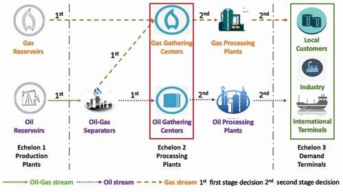
HCSC extends from crude oil and natural gas production fields, goes through processing and transforming operations, and ends at demand terminals. Attia, Ghaithan, and Duffuaa (2019a) provides a detailed description of the different activities and products of the HCSC. There is an overlap between crude oil and natural gas SCs because of the inclusion of associated gas in crude oil. A schematic representation of the network is depicted in Figure 1.

The produced crude oil is transported to gas-oil separator plants (GOSPs). The separated oil is then gathered and transported to the oil processing plants for stabilisation and sweetening (i.e. removing H₂S and other gases). At the same time, the separated gas (i.e. associated gas) and non-associated gas are collected at the gas gathering centres. The gas is then processed to remove H₂S and CO₂, while methane and natural gas liquid (NGL) are produced. Furthermore, the NGL is further processed to produce different gas products (e.g. ethane, butane, propane, and natural gasoline). Eventually, the processed crude oil and gas products are transported to different demand terminals (e.g. local, industrial, and international).

Figure 1. HCSC activities and decisions of 1^st and 2^nd stages

3.1. Uncertainties in HCSC

Model parameters are classified as either certain or uncertain. Certain parameters are defined as those determined by the decision-maker beforehand (e.g. OPEC quota, gas-oil ratio (GOR), CO₂ emission limit). While uncertain parameters cannot be determined (e.g. yield) or may change as a result of market behaviour (e.g. price and demand). In real-life situations, the values of uncertain parameters are not known at the start of the planning period. Consequently, the decision-maker has to make some decisions based on the known values of certain parameters; then, as the realisation of some uncertain parameters becomes clear, he/she can take the second batch of decisions (recourse decisions). This process continues (i.e. decide, realise, decide, realise, and so on) until all parameters are recognised, and all decisions are taken. Thus, the multi-stage SP can model the previous process involving staged decision-making.

Price and demand at echelon 3 are considered uncertain parameters in this study, while other parameters are assumed to be known and fixed. The reason behind price selection is the dramatic fluctuations in crude oil and petroleum products prices in recent years. Uncertain parameters can be represented by a plausible number of scenarios (i.e. finite set of realisations) with corresponding probabilities of occurrence.

At the start of the planning period, certain parameters are known in a two-stage SP, while uncertain parameters are subsequently realised. Figure 1 depicts the HCSC’s first and second stage decisions, such that the production from the oil and gas reservoirs starts at the beginning, as early as possible, to ensure satisfying the demand on time. The produced oil and gas, associated and non-associated, are then stored in the gathering centres. After that, the market scenarios for price and demand became known. Consequently, sufficient quantities are extracted from the gathering centres for further processing, transformation, and distribution. Extraction from gathering centres is known as recourse or corrective action, and it occurs when not all the produced quantities are sent for further activities (i.e. quantities as per need based on scenario values).

Dantzig (1955) proposed the first representation of the two-stage SP model. The following formulation is adopted from (Conejo, Carrión, and Morales 2010):

(1) $Minimiz{e}_{x}z=c^{T}x+E\left\{Q\left(\omega \right)\right\}$(1)

(2) $subjecttoAx=b$(2)

(3) $x\in X$(3)

(4) $Q\left(\omega \right)=\left\{minimiz{e}_{y\left(\omega \right)}q{\left(\omega \right)}^{T}y\left(\omega \right)\right.$(4)

(5) $subjecttoT\left(\omega \right)x+W\left(\omega \right)y\left(\omega \right)=h\left(\omega \right)$(5)

(6) $\left.y\left(\omega \right)\in Y\right\},\omega \in \mathrm{\Omega }$(6)

Where x and y(ω) are the first- and second-stage decisions, ω scenario index, is the expected value of the second-stage decisions. The deterministic equivalent of the above formulation after a rearrangement is as follows:

(7) $Minimiz{e}_{x,y\left(\omega \right)}z=c^{T}x+\sum _{\omega \in \mathrm{\Omega }}\pi \left(\omega \right)q{\left(\omega \right)}^{T}y\left(\omega \right)$(7)

(8) $subjecttoAx=b$(8)

(9) $T\left(\omega \right)x+W\left(\omega \right)y\left(\omega \right)=h\left(\omega \right),\omega \in \mathrm{\Omega }$(9)

(10) $x\in X,y\left(\omega \right)\in Y,\omega \in \mathrm{\Omega }$(10)

3.2. Model notations

Table 1 summarises the definition of the sets, parameters, and variables used to formulate the proposed model, mainly adopted from (Attia, Ghaithan, and Duffuaa 2019a).

Table 1. Model notations

Sets/Indices:
$i,j:$	all nodes.
$RO,RG:$	set of (oil, gas) reservoirs, denoted by indices $\left(ro,rg\right)$.
$N:$	set of GOSPs, denoted by index $n$.
$GO,GG:$	set of (oil, gas) gathering centres, denoted by indices $\left(go,gg\right)$.
$PO,PG:$	set of (oil, gas) processing plants, denoted by indices $\left(po,pg\right)$.
$DO,DG:$	set of (oil, gas) demand terminals, denoted by indices $\left(do,dg\right)$.
$LOCO,LOCG:$	a subset of $\left(DO,DG\right)$ represents (oil, gas) local depots, denoted by indices $\left(loco,locg\right)$.
$INDO,INDG:$	a subset of $\left(DO,DG\right)$ represents (oil, gas) industrial complexes, denoted by indices $\left(indo,indg\right)$.
$INTO,INTG:$	a subset of $\left(DO,DG\right)$ represents (oil, gas) international terminals, denoted by indices $\left(into,intg\right)$.
$\mathrm{\Omega }:$	set of scenarios, denoted by index $\omega$.
$\pi \left(\omega \right):$	probability of scenario$\omega$.
$O:$	set of crude oil types, denoted by index $o$; e.g. AH Arabian Heavy Crude, AM Arabian Medium Crude, AL Arabian Light Crude, and AXL Arabian Extra Light Crude.
$G:$	set of natural gas byproducts, denoted by index $g$; includes subsets: GN natural gas with index $gn$, GP gas byproducts produced at processing plants with index $gp$, H2S and CO2.
$T:$	set of periods with index t.
Decision Variables:
First stage decisions:
$x_{ijt}^{1o}:$	amount of crude oil of type o produced in period t transported from node i to node j, Mbarrel/period; where $\left(i,j\right)\in \left(ro,n\right),\left(n,go\right)$.
$y_{ijt}^{1g}:$	amount of natural gas of type g produced in period t transported from node i to node j, Mcft/period; where $\left(i,j\right)\in \left(rg,gg\right),\left(n,gg\right)$.
$D:$	depletion rate of the reserves (i.e. crude oil and gas).
Second stage decisions:
$x_{ij\omega t}^{2o}:$	amount of crude oil of type o produced in period t under scenario ω transported from node i to node j, Mbarrel/period; where $\left(i,j\right)\in \left(go,po\right),\left(po,do\right)$.
$y_{ij\omega t}^{2g}:$	amount of natural gas of type g produced in period t under scenario ω transported from node i to node j, Mcft/period; where $\left(i,j\right)\in \left(gg,pg\right),\left(pg,dg\right)$.
$x_{j\omega t}^{2o+}:$	crude oil production of type o in period t under scenario ω above the demand at node j, Mbarrel/period; where $j\in go,do.$
$x_{j\omega t}^{2o-}:$	crude oil production of type o in period t under scenario ω below the demand at node j (i.e. satisfied from the outside market), Mbarrel/period; where $j\in go,do$.
$y_{j\omega t}^{2g+}:$	gas production of product g in period t under scenario ω above the demand at node j, Mcft/period; where $\mathrm{j}\in gg,dg$.
$y_{j\omega t}^{2g-}:$	gas production of product g in period t under scenario ω below the demand at node j (i.e. satisfied from the outside market), Mcft/period; where $\mathrm{j}\in gg,dg$.
Parameters:
Yield parameters:
$GO{R}_{ijt}^o:$	Gas-oil ratio of crude oil type o produced during period t from reservoir i linked to GOSP j; where $\left(i,j\right)\in \left(ro,n\right)$.
$P_{ijt}^o:$	yield of crude oil of type o liberated during period t at node i transported to node j, percentage; where $\left(i,j\right)\in \left(ro,n\right),\left(go,po\right)$.
$P_{ijt}^g:$	yield of gas product g obtained during period t at node i transported to node j, percentage; where$\left(i,j\right)\in \left(gg,pg\right)$.
Capacity parameters:
$C_j^o:$	capacity of node j for crude oil o, Mbarrel/period; where$j\in n,go,po,do$.
$C_j^g:$	capacity of node j for gas product g, Mcft/period; where$j\in gg,pg,dg$.
$c_{ij}^o:$	capacity of the route linking node i to node j of crude oil o, Mbarrel/period; where $\left(i,j\right)\in \left(ro,n\right),\left(n,go\right),\left(go,po\right),\left(po,do\right)$.
$c_{ij}^g:$	capacity of the route linking node i to node j for gas product g, Mcft/period; where $\left(i,j\right)\in \left(rg,gg\right),\left(n,gg\right),\left(gg,pg\right),\left(pg,dg\right)$.
Volume parameters:
$R_i^o:$	amount of reserves in reservoir at node i for oil type o, Mbarrel/period; where$i\in ro$.
$R_i^g:$	amount of reserves in reservoir at node i for gas g, Mcft/period; where$i\in rg$.
$C_{max}:$	maximum amount of CO2 to be emitted to the environment in period t, Mbarrel/period.
$OPECQ:$	OPEC quota or market share per planning period t, Mbarrel/period.
Cost parameters:
$e{c}_{ijt}^o:$	production cost per unit of stream $x_{ijt}^{1o}$, at node i during period t, $/barrel; where $\left(i,j\right)\in \left(ro,n\right)$.
$e{c}_{ijt}^g:$	production cost per unit of stream $y_{ijt}^{1g}$, at node i during period t, $/cft; where $\left(i,j\right)\in \left(rg,gg\right)$.
$p{c}_{ijt}^o:$	processing cost per unit of stream $x_{ijt}^{1o}and{x}_{ij\omega t}^{2o}$, at node j during period t, $/barrel; where $\left(i,j\right)\in \left(ro,n\right),\left(go,po\right)$.
$p{c}_{ijt}^g:$	processing cost per unit of stream $y_{ijt}^{1g}and{y}_{ij\omega t}^{2g}$, at node j during period t, $/cft; where $\left(i,j\right)\in \left(gg,pg\right)$.
$t{c}_{ijt}^o:$	transportation cost per unit of stream $x_{ijt}^{1o}and{x}_{ij\omega t}^{2o}$, from node i to node j during period t, $/barrel; where $\left(i,j\right)\in \left(ro,n\right),\left(n,go\right),\left(go,po\right),\left(\mathrm{p}\mathrm{o},\mathrm{d}\mathrm{o}\right)$.
$t{c}_{ijt}^g:$	transportation cost per unit of stream $y_{ijt}^{1g}and{y}_{ij\omega t}^{2g}$, from node i to node j during period t, $/cft; where $\left(i,j\right)\in \left(rg,gg\right),\left(n,gg\right),\left(gg,pg\right),\left(pg,dg\right)$.
$c_{jt}^g:$	cost per unit of emitting CO2 to the environment at plant i during period t, $/cft; where $j\in pg$.
$w_{j\omega t}^{o+}:$	penalty cost per unit for producing crude oil of type o above the specified demand at node j during period t, $/barrel; $wherej\in go,do$.
$w_{j\omega t}^{o-}:$	penalty cost per unit for producing crude oil of type o below the specified demand at node j during period t (i.e. penalty of filling part of the demand from the outside market), $/barrel; $wherej\in go,do$.
$w_{j\omega t}^{g+}:$	penalty cost per unit for producing gas product g above the specified demand at node j during period t, $/cft; $wherej\in gg,dg$.
$w_{j\omega t}^{g-}:$	penalty cost per unit for producing gas product g below the specified demand at node j during period t (i.e. penalty of filling part of the demand from the outside market), $/cft; $wherej\in gg,dg$.
Demand and prices parameters:
$d_{j\omega t}^o:$	demand at destination j for crude oil of type o under scenario ω in period t, Mbarrel/period; where $j\in do$.
$d_{j\omega t}^g:$	demand at destination j for gas product g under scenario ω in period t, Mcft/period; where $j\in dg$.
$p{r}_{j\omega t}^o:$	selling price per unit of crude oil type o during period t under scenario ω at demand node j, $/barrel; where $j\in do$.
$p{r}_{j\omega t}^g:$	Selling price per unit of gas products g during period t under scenario ω at demand node j, $/cft; where $j\in dg$.
$dr:$	Discount rate per period t.

3.3. Model constraints

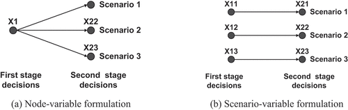
Constraints and objective functions in SP can be formulated mathematically based on either node-variable formulation or scenario-variable formulation (Conejo, Carrión, and Morales 2010), as represented in Figure 2. In node-variable formulation, the number of decision variables depends on the number of decision points, whereas a scenario-based formulation depends on the number of scenarios. Node-variable formulation generates a compact model and utilises the recent advances in commercial software for solving optimization models without decomposition. In contrast, scenario-based formulation generates relatively larger models that are naturally decomposed. In this work, the model is formulated based on node-variable formulation.

Figure 2. SP formulation methods

There are eight sets of constraints formulated considering scenarios, ω, of uncertain parameters in addition to 1^st and 2^nd stage decision variables.

(1) Material balance constraints of the 2^nd echelon plants: Equatios (11)(11) $\sum _{i\in ro}{P}_{ijt}^o{x}_{ijt}^{1o}=\sum _{i\in go}{x}_{jit}^{1o}\mathrm{\forall }o,\mathrm{\forall }j\in n$(11) and (12(12) $\sum _{i\in ro}GO{R}_{ijt}^o{x}_{ijt}^{1o}=\sum _{i\in gg}{y}_{jit}^{1g}\mathrm{\forall }o,\mathrm{\forall }j\in n$(12) ) formulate the material balance at GOSPs, n, for crude oil and associated gas. The input stream, $x_{ijt}^{1o}$, output oil stream, $x_{jit}^{1o}$, and output gas stream, $y_{jit}^{1g}$, are 1^st stage decisions. The output oil stream depends on the yield, $P_{ijt}^o$, and the output associated gas stream depends on the gas-oil ratio, $GO{R}_{ijt}^o$. The material balance at the oil, PO, and gas, PG processing plants, represented by Equations (14)(14) $\sum _{i\in go}{P}_{ij}^o{x}_{ij\omega t}^{2o}=\sum _{i\in do}{x}_{ji\omega t}^{2o}\mathrm{\forall }o,\mathrm{\forall }j\in po,\mathrm{\forall }\omega$(14) and (15(15) $\sum _{i\in go}{P}_{ij}^o{x}_{ij\omega t}^{2o}=\sum _{g\in H2S;i\in dg}{y}_{ji\omega t}^{2g}\mathrm{\forall }o,\mathrm{\forall }j\in po,\mathrm{\forall }\omega$(15) ), and Equation (17)(17) $\sum _{i\in gg}{P}_{ijt}^g{y}_{ij\omega t}^{2g}=\sum _{i\in dg}{y}_{ij\omega t}^{2g}\mathrm{\forall }g,\mathrm{\forall }j\in pg,\mathrm{\forall }\omega$(17) for oil and gas, respectively. Equations (14)(14) $\sum _{i\in go}{P}_{ij}^o{x}_{ij\omega t}^{2o}=\sum _{i\in do}{x}_{ji\omega t}^{2o}\mathrm{\forall }o,\mathrm{\forall }j\in po,\mathrm{\forall }\omega$(14) and (15(15) $\sum _{i\in go}{P}_{ij}^o{x}_{ij\omega t}^{2o}=\sum _{g\in H2S;i\in dg}{y}_{ji\omega t}^{2g}\mathrm{\forall }o,\mathrm{\forall }j\in po,\mathrm{\forall }\omega$(15) ) receive oil, $x_{ij\omega t}^{2o}$, and produce oil, $x_{ji\omega t}^{2o}$, and gas, $y_{ji\omega t}^{2g}$, based on the input stream yield characteristics, $P_{ij}^o$. Beside Equations (13)(13) $\sum _{i\in n}{x}_{ijt}^{1o}+x_{j\omega t-1}^{2o+}=\sum _{i\in po}{x}_{ji\omega t}^{2o}+x_{j\omega t}^{2o+}\mathrm{\forall }o,\mathrm{\forall }j\in go,\mathrm{\forall }\omega$(13) and (16(16) $\sum _{i\in rg}{y}_{ijt}^{1g}+\sum _{i\in n}{y}_{ijt}^{1g}+y_{j\omega t-1}^{2g+}=\sum _{i\in pg}{y}_{ji\omega t}^{2g}+y_{j\omega t}^{2g+}\mathrm{\forall }g,\mathrm{\forall }j\in gg,\mathrm{\forall }\omega$(16) ) balance the material at the oil, go, and gas, gg, gathering centres by receiving the input from GOSPs, n, and gas reservoirs, rg, then the output sent to the oil, po, and gas, pg, processing plants. The output from the gathering centres is scenario-based, ω.

(11) $\sum _{i\in ro}{P}_{ijt}^o{x}_{ijt}^{1o}=\sum _{i\in go}{x}_{jit}^{1o}\mathrm{\forall }o,\mathrm{\forall }j\in n$(11)

(12) $\sum _{i\in ro}GO{R}_{ijt}^o{x}_{ijt}^{1o}=\sum _{i\in gg}{y}_{jit}^{1g}\mathrm{\forall }o,\mathrm{\forall }j\in n$(12)

(13) $\sum _{i\in n}{x}_{ijt}^{1o}+x_{j\omega t-1}^{2o+}=\sum _{i\in po}{x}_{ji\omega t}^{2o}+x_{j\omega t}^{2o+}\mathrm{\forall }o,\mathrm{\forall }j\in go,\mathrm{\forall }\omega$(13)

(14) $\sum _{i\in go}{P}_{ij}^o{x}_{ij\omega t}^{2o}=\sum _{i\in do}{x}_{ji\omega t}^{2o}\mathrm{\forall }o,\mathrm{\forall }j\in po,\mathrm{\forall }\omega$(14)

(15) $\sum _{i\in go}{P}_{ij}^o{x}_{ij\omega t}^{2o}=\sum _{g\in H2S;i\in dg}{y}_{ji\omega t}^{2g}\mathrm{\forall }o,\mathrm{\forall }j\in po,\mathrm{\forall }\omega$(15)

(16) $\sum _{i\in rg}{y}_{ijt}^{1g}+\sum _{i\in n}{y}_{ijt}^{1g}+y_{j\omega t-1}^{2g+}=\sum _{i\in pg}{y}_{ji\omega t}^{2g}+y_{j\omega t}^{2g+}\mathrm{\forall }g,\mathrm{\forall }j\in gg,\mathrm{\forall }\omega$(16)

(17) $\sum _{i\in gg}{P}_{ijt}^g{y}_{ij\omega t}^{2g}=\sum _{i\in dg}{y}_{ij\omega t}^{2g}\mathrm{\forall }g,\mathrm{\forall }j\in pg,\mathrm{\forall }\omega$(17)

(2) Plant capacity constraints of the 2^nd and 3^rd echelon plants: Equations (18)(18) $\sum _{i\in ro}{p}_{ijt}^o{x}_{ijt}^{1o}\le C_j^o\mathrm{\forall }o,\mathrm{\forall }j\in n$(18) –(21(21) $\sum _{i\in po}{x}_{ij\omega t}^{2o}+x_{j\omega t-1}^{2o+}\le C_j^o\mathrm{\forall }o,\mathrm{\forall }j\in do,\mathrm{\forall }\omega$(21) ) represent the maximum processing capacity of oil plants: reservoirs, ro, GOSPs, n, gathering centres, go, processing plants, po, and demand terminals, do, respectively. Equations (22)(22) $\sum _{i\in rg}{y}_{ijt}^{1g}+\sum _{i\in n}{y}_{ijt}^{1g}+y_{j\omega t-1}^{2g+}\le C_j^g\mathrm{\forall }g,\mathrm{\forall }j\in gg,\mathrm{\forall }\omega$(22) , (23(23) $\sum _{i\in gg}{p}_{ijt}^g{y}_{ij\omega t}^{2g}\le C_j^g\mathrm{\forall }g,\mathrm{\forall }j\in pg,\mathrm{\forall }\omega$(23) ), and (24(24) $\sum _{i\in pg}{y}_{ij\omega t}^{2g}+y_{j\omega t-1}^{2g+}\le C_j^g\mathrm{\forall }g,\mathrm{\forall }j\in dg,\mathrm{\forall }\omega$(24) ) model the capacity of gas plants.

(3) Route capacity constraints: connecting all the plants are represented in Equations (25)(25) $x_{ijt}^{1o}\le c_{ij}^o\mathrm{\forall }o,\mathrm{\forall }\left(i,j\right)\in \left(ro,n\right),\left(n,go\right)$(25) and (27(27) $y_{ijt}^{1g}\le c_{ij}^g\mathrm{\forall }g,\mathrm{\forall }\left(i,j\right)\in \left(rg,gg\right)$(27) ) for 1^st stage decisions and Equations (26)(26) $x_{ij\omega t}^{2o}\le c_{ij}^o\mathrm{\forall }o,\mathrm{\forall }\left(i,j\right)\in \left(go,po\right),\left(po,do\right),\mathrm{\forall }\omega$(26) and (28(28) $y_{ij\omega t}^{2g}\le c_{ij}^g\mathrm{\forall }g,\mathrm{\forall }\left(i,j\right)\in \left(gg,pg\right),\left(pg,dg\right),\mathrm{\forall }\omega$(28) ) for 2^nd stage decisions.

(18) $\sum _{i\in ro}{p}_{ijt}^o{x}_{ijt}^{1o}\le C_j^o\mathrm{\forall }o,\mathrm{\forall }j\in n$(18)

(19) $\sum _{i\in n}{x}_{ijt}^{1o}+x_{j\omega t-1}^{2o+}\le C_j^o\mathrm{\forall }o,\mathrm{\forall }j\in go,\mathrm{\forall }\omega$(19)

(20) $\sum _{i\in go}{p}_{ijt}^o{x}_{ij\omega t}^{2o}\le C_j^o\mathrm{\forall }o,\mathrm{\forall }j\in po,\mathrm{\forall }\omega$(20)

(21) $\sum _{i\in po}{x}_{ij\omega t}^{2o}+x_{j\omega t-1}^{2o+}\le C_j^o\mathrm{\forall }o,\mathrm{\forall }j\in do,\mathrm{\forall }\omega$(21)

(22) $\sum _{i\in rg}{y}_{ijt}^{1g}+\sum _{i\in n}{y}_{ijt}^{1g}+y_{j\omega t-1}^{2g+}\le C_j^g\mathrm{\forall }g,\mathrm{\forall }j\in gg,\mathrm{\forall }\omega$(22)

(23) $\sum _{i\in gg}{p}_{ijt}^g{y}_{ij\omega t}^{2g}\le C_j^g\mathrm{\forall }g,\mathrm{\forall }j\in pg,\mathrm{\forall }\omega$(23)

(24) $\sum _{i\in pg}{y}_{ij\omega t}^{2g}+y_{j\omega t-1}^{2g+}\le C_j^g\mathrm{\forall }g,\mathrm{\forall }j\in dg,\mathrm{\forall }\omega$(24)

(25) $x_{ijt}^{1o}\le c_{ij}^o\mathrm{\forall }o,\mathrm{\forall }\left(i,j\right)\in \left(ro,n\right),\left(n,go\right)$(25)

(26) $x_{ij\omega t}^{2o}\le c_{ij}^o\mathrm{\forall }o,\mathrm{\forall }\left(i,j\right)\in \left(go,po\right),\left(po,do\right),\mathrm{\forall }\omega$(26)

(27) $y_{ijt}^{1g}\le c_{ij}^g\mathrm{\forall }g,\mathrm{\forall }\left(i,j\right)\in \left(rg,gg\right)$(27)

(28) $y_{ij\omega t}^{2g}\le c_{ij}^g\mathrm{\forall }g,\mathrm{\forall }\left(i,j\right)\in \left(gg,pg\right),\left(pg,dg\right),\mathrm{\forall }\omega$(28)

(4) Demand constraints at the 3^rd echelon: Equations (29)(29) $\sum _{i\in po}{x}_{ij\omega t}^{2o}-x_{j\omega t}^{2o+}+x_{j\omega t}^{2o-}=d_{j\omega t}^o-x_{j\omega t-1}^{2o+}\mathrm{\forall }o,\mathrm{\forall }j\in do,\mathrm{\forall }\omega$(29) and (30(30) $\sum _{i\in pg}{y}_{ij\omega t}^{2g}-y_{j\omega t}^{2g+}+y_{j\omega t}^{2g-}=d_{j\omega t}^g-y_{j\omega t-1}^{2g+}\mathrm{\forall }g,\mathrm{\forall }j\in dg,\mathrm{\forall }\omega$(30) ). (5) OPEC quota constraint at the 3^rd echelon: Equation (31)(31) $\sum _{o,i\in po,j\in into}{x}_{ij\omega t}^{2o}+\sum _{o;j\in into}{x}_{jt-1}^{o+}\le OPECQ\mathrm{\forall }\omega$(31) , and (6) Environmental regulations constraints at gas processing plants: Equation (32)(32) $\sum _{g\in CO2;j\in pg}{y}_{j\omega t}^{2g}\le C_{max}\mathrm{\forall }\omega$(32) based on 2^nd stage decisions. (7) Sustainability constraints at 1^st echelon plants: Equations (33)(33) $\frac{{\sum }_{i\in ro,j\in n}{x}_{ijt}^{1o}}{{\sum }_{c,i\in ro}{R}_{it}^o}\le D$(33) and (34(34) $\frac{{\sum }_{i\in rg,j\in gg}{y}_{ijt}^{1g}}{{\sum }_{g,i\in rg}{R}_{it}^g}\le D$(34) ) depend on first-stage decisions. Eventually, (8) Non-negativity constraints: Equations (35)(35) $x_{ijt}^{1o},x_{ij\omega t}^{2o},x_{j\omega t}^{2o+},x_{j\omega t}^{2o-},y_{ijt}^{2g},y_{ij\omega t}^{2g},y_{j\omega t}^{2g+},y_{j\omega t}^{2g-},D\ge 0$(35) .

(29) $\sum _{i\in po}{x}_{ij\omega t}^{2o}-x_{j\omega t}^{2o+}+x_{j\omega t}^{2o-}=d_{j\omega t}^o-x_{j\omega t-1}^{2o+}\mathrm{\forall }o,\mathrm{\forall }j\in do,\mathrm{\forall }\omega$(29)

(30) $\sum _{i\in pg}{y}_{ij\omega t}^{2g}-y_{j\omega t}^{2g+}+y_{j\omega t}^{2g-}=d_{j\omega t}^g-y_{j\omega t-1}^{2g+}\mathrm{\forall }g,\mathrm{\forall }j\in dg,\mathrm{\forall }\omega$(30)

(31) $\sum _{o,i\in po,j\in into}{x}_{ij\omega t}^{2o}+\sum _{o;j\in into}{x}_{jt-1}^{o+}\le OPECQ\mathrm{\forall }\omega$(31)

(32) $\sum _{g\in CO2;j\in pg}{y}_{j\omega t}^{2g}\le C_{max}\mathrm{\forall }\omega$(32)

(33) $\frac{{\sum }_{i\in ro,j\in n}{x}_{ijt}^{1o}}{{\sum }_{c,i\in ro}{R}_{it}^o}\le D$(33)

(34) $\frac{{\sum }_{i\in rg,j\in gg}{y}_{ijt}^{1g}}{{\sum }_{g,i\in rg}{R}_{it}^g}\le D$(34)

(35) $x_{ijt}^{1o},x_{ij\omega t}^{2o},x_{j\omega t}^{2o+},x_{j\omega t}^{2o-},y_{ijt}^{2g},y_{ij\omega t}^{2g},y_{j\omega t}^{2g+},y_{j\omega t}^{2g-},D\ge 0$(35)

3.4. Model objective functions

Three objective functions have been proposed to investigate the trade-off between different economic and non-economic objectives. (1) Total cost minimization: expressed in Equation (36)(36) $\begin{array}{rl}& MinimizeTotalCost=\sum _t{\left(1+dr\right)}^{-\left(t-1\right)}\left[\sum _{o,\left(i,j\right)\in \left(ro,n\right)}e{c}_{ijt}^o{x}_{ijt}^{1o}\right.+\sum _{g,\left(i,j\right)\in \left(rg,gg\right)}e{c}_{ijt}^g{y}_{ijt}^{1g}\\ & +\sum _{o,\left(i,j\right)\in \left(ro,n\right)}t{c}_{ijt}^o{x}_{ijt}^{1o}+\sum _{g,\left(i,j\right)\in \left(rg,gg\right)}t{c}_{ijt}^g{y}_{ijt}^{1g}\\ & +\sum _{o,\left(i,j\right)\in \left(ro,n\right)}p{c}_{ijt}^o{x}_{ijt}^{1o}\\ & +\sum _{\omega }{\pi }_{\omega }\left(\sum _{o,\left(i,j\right)\in \left(go,po\right)}p{c}_{ijt}^o{x}_{ij\omega t}^{2o}+\sum _{g,\left(i,j\right)\in \left(gg,pg\right)}p{c}_{ijt}^g{y}_{ij\omega t}^{2g}\right.\\ & +\sum _{o,\left(i,j\right)\in \left(n,po\right),\left(po,do\right)}t{c}_{ijt}^o{x}_{ij\omega t}^{2o}+\sum _{g,\left(i,j\right)\in \left(gg,pg\right),\left(pg,dg\right)}t{c}_{ijt}^g{y}_{ij\omega t}^{2g}\\ & +\sum _{o,j\in \left(go,do\right)}\left(w_{j\omega }^{o+}{x}_{j\omega t}^{2o+}+w_{j\omega }^{o-}{x}_{j\omega t}^{2o-}\right)+\sum _{g,j\in \left(gg,dg\right)}\left(w_{j\omega }^{g+}{y}_{j\omega t}^{2g+}+w_{j\omega }^{g-}{y}_{j\omega t}^{2g-}\right)\\ & \left.\left.+\sum _{g\in CO2;j\in pg}{c}_{it}^g{y}_{j\omega t}^{2g}\right)\right]\end{array}$(36) . The considered costs are production costs at the 1^st echelon represented by terms 1 and 2, the processing cost at the 2^nd echelon plants represented by terms 5, 6, and 7, the transportation costs represented by terms 3, 4, 8, and 9, holding costs at gathering centres represented by terms 10 and 11 t, the penalty cost of producing over-or under- the demand represented by terms 10 and 11, and the final term account for CO2 emissions cost.

(2) Total revenue maximization: computed by subtracting the amount of production above the demand (i.e. over-production that cannot be sold) from total production results in the actual selling amount, equal to the demand, formulated in Equation (37)(37) $\begin{array}{rl}& \mathrm{m}\mathrm{a}\mathrm{x}\mathrm{i}\mathrm{m}\mathrm{i}\mathrm{z}\mathrm{e}Revenue=\\ & \sum _t{\left(1+dr\right)}^{-\left(t-1\right)}\left[\sum _{\omega }{\pi }_{\omega }\left(\sum _{o,\left(i,j\right)\in \left(po,do\right)}p{r}_{j\omega t}^o\left(x_{ij\omega t}^{2o}-x_{j\omega t}^{2o+}\right)\right.\right.\\ & \left.\left.+\sum _{g,\left(i,j\right)\in \left(pg,dg\right)}p{r}_{j\omega t}^g\left(y_{ij\omega t}^{2g}-y_{j\omega t}^{2g+}\right)\right)\right]\end{array}$(37) . The total cost and revenue are discounted back to their present value based on the discount rate dr per planning period t. (3) Depletion rate minimization: formulated in Equation (38)(38) $\mathrm{m}\mathrm{i}\mathrm{n}\mathrm{i}\mathrm{m}\mathrm{i}\mathrm{z}\mathrm{e}D$(38) as a ratio of production from reservoirs to the total proved reserves. Therefore, the proposed model can maximize the sustainability of the reserves of natural resources (e.g. crude oil and natural gas).

(36) $\begin{array}{rl}& MinimizeTotalCost=\sum _t{\left(1+dr\right)}^{-\left(t-1\right)}\left[\sum _{o,\left(i,j\right)\in \left(ro,n\right)}e{c}_{ijt}^o{x}_{ijt}^{1o}\right.+\sum _{g,\left(i,j\right)\in \left(rg,gg\right)}e{c}_{ijt}^g{y}_{ijt}^{1g}\\ & +\sum _{o,\left(i,j\right)\in \left(ro,n\right)}t{c}_{ijt}^o{x}_{ijt}^{1o}+\sum _{g,\left(i,j\right)\in \left(rg,gg\right)}t{c}_{ijt}^g{y}_{ijt}^{1g}\\ & +\sum _{o,\left(i,j\right)\in \left(ro,n\right)}p{c}_{ijt}^o{x}_{ijt}^{1o}\\ & +\sum _{\omega }{\pi }_{\omega }\left(\sum _{o,\left(i,j\right)\in \left(go,po\right)}p{c}_{ijt}^o{x}_{ij\omega t}^{2o}+\sum _{g,\left(i,j\right)\in \left(gg,pg\right)}p{c}_{ijt}^g{y}_{ij\omega t}^{2g}\right.\\ & +\sum _{o,\left(i,j\right)\in \left(n,po\right),\left(po,do\right)}t{c}_{ijt}^o{x}_{ij\omega t}^{2o}+\sum _{g,\left(i,j\right)\in \left(gg,pg\right),\left(pg,dg\right)}t{c}_{ijt}^g{y}_{ij\omega t}^{2g}\\ & +\sum _{o,j\in \left(go,do\right)}\left(w_{j\omega }^{o+}{x}_{j\omega t}^{2o+}+w_{j\omega }^{o-}{x}_{j\omega t}^{2o-}\right)+\sum _{g,j\in \left(gg,dg\right)}\left(w_{j\omega }^{g+}{y}_{j\omega t}^{2g+}+w_{j\omega }^{g-}{y}_{j\omega t}^{2g-}\right)\\ & \left.\left.+\sum _{g\in CO2;j\in pg}{c}_{it}^g{y}_{j\omega t}^{2g}\right)\right]\end{array}$(36)

(37) $\begin{array}{rl}& \mathrm{m}\mathrm{a}\mathrm{x}\mathrm{i}\mathrm{m}\mathrm{i}\mathrm{z}\mathrm{e}Revenue=\\ & \sum _t{\left(1+dr\right)}^{-\left(t-1\right)}\left[\sum _{\omega }{\pi }_{\omega }\left(\sum _{o,\left(i,j\right)\in \left(po,do\right)}p{r}_{j\omega t}^o\left(x_{ij\omega t}^{2o}-x_{j\omega t}^{2o+}\right)\right.\right.\\ & \left.\left.+\sum _{g,\left(i,j\right)\in \left(pg,dg\right)}p{r}_{j\omega t}^g\left(y_{ij\omega t}^{2g}-y_{j\omega t}^{2g+}\right)\right)\right]\end{array}$(37)

(38) $\mathrm{m}\mathrm{i}\mathrm{n}\mathrm{i}\mathrm{m}\mathrm{i}\mathrm{z}\mathrm{e}D$(38)

4. Solution methodology

The adopted solution methodology uses an improved version of the ε-constraint approach introduced by (Mavrotas and Florios 2013) to produce the Pareto-optima. The preferred plan from Pareto-optima set is chosen using Technique by Similarity to Ideal Solution (TOPSIS).

4.1. Multi-objective optimization

AUGMECON 2 (augmented epsilon constraint 2) is a modified version of the ε-constraint method proposed by (Mavrotas and Florios 2013) used to generate the Pareto-optima. The algorithm for the three objective functions is as the following:

Step 1: Identify the range of each objective function to establish the pay-off matrix and apply the Lexicographic optimization:

1. Minimize the total cost, f1, ignoring the other two objectives, f2 and f3, and be subject to all constraints.

2. Maximize the total revenue, f2, consider f1 as an equality constraint and be subject to all constraints.

3. Minimize the depletion rate, f3, consider f1 and f2 as equality constraints, and be subject to all constraints.

Step 2: Repeat step 1 by changing the order of the objective functions.

Step 3: Generate the Pareto-optima.

1. Choose f1 as a primary objective and divide the range of f2 and f3 equidistantly.

2. Try different resolutions of f2 and f3 and choose the best one based on the maximum Euclidean distance between the successive resolutions.

3. Apply an exhaustive enumeration over (f1, f2, f3) and obtain the corresponding decision variables.

4.2. Preferred plan selection

Pareto-optima is a finite number of tactical plans; thus, the problem is to find the preferred plan among a finite number of feasible plans based on conflicting criteria. This technique is a multi-criteria decision-making (MCDM), and TOPSIS is a numerical method used to solve this problem (Clemen and Reilly 2004; Tzeng and Huang 2011). The steps of the TOPSIS method is as follows (Ewa 2011)

Step 1: Construct the decision matrix and determine the weight of criteria, w, as shown in Table 2.

Table 2. Alternative decision matrix

		Criteria (Objective functions)
	Weight	w1	w2	w3
		f1	f2	f3
Alternatives	A1	x11	x12	x13
	A2	x21	x22	x23
	…	…	…	…
	Am	xn1	xn2	xn3

Step 2: Calculate the normalised decision matrix

(39) $n_{ij}=\frac{x_{ij}}{\sqrt{{\sum }_{i=1}^m{x}_{ij}}};i=1,\dots ,m;j=1,2,3$(39)

Step 3: Calculate the weighted normalised decision matrix

(40) $v_{ij}=w_{ij}{n}_{ij};i=1,\dots ,m;j=1,2,3;\sum _{j=1}^3{w}_j=1$(40)

Step 4: Determine the positive ideal and negative ideal solutions.

Positive ideal solution A⁺, best values on each criterion, has the form:

(41) $A^{+}=\left(v_1^{+},v_2^{+},v_3^{+}\right)=\left(\left(\left.\underset{i}{max{v}_{ij}}\right|j\in J\right),\left(\left.\underset{i}{min{v}_{ij}}\right|j\in J\right)\right)$(41)

Negative ideal solution A⁻, worst values on each criterion, has the form:

(42) $A^{-}=\left(v_1^{-},v_2^{-},v_3^{-}\right)=\left(\left(\left.\underset{i}{min{v}_{ij}}\right|j\in J\right),\left(\left.\underset{i}{max{v}_{ij}}\right|j\in J\right)\right)$(42)

Step 5: Calculate the separation measures from the positive ideal solution and the negative ideal solution.

(43) $d_i^{+}=\sqrt{\sum _{j=1}^n{\left(v_{ij}-v_j^{+}\right)}^2};i=1,\dots ,m$(43)

(44) $d_i^{-}=\sqrt{\sum _{j=1}^n{\left(v_{ij}-v_j^{-}\right)}^2};i=1,\dots ,m$(44)

Step 6: Calculate the relative closeness to the positive ideal solution.

(45) $R_i=\frac{d_i^{-}}{d_i^{-}+d_i^{+}};0\le R_i\le 1;i=1,\dots ,m$(45)

Step 7: Rank the preference order or select the alternative closest to 1.

5. Case study

The Saudi Arabian HCSC was utilised to evaluate the proposed model’s practicability and performance. This section presents the analysis of the results and highlights managerial insights after conducting the sensitivity analysis.

5.1. Saudi Arabian HCSC

The production areas, processing plants, and demand terminals of the HCSC are shown in Figures 3 and Figures 4 based on (McMurra 2011; Attia, Ghaithan, and Duffuaa 2019b, 2019a). Saudi Arabia produces crude oil in 4 different types: AXL, AL, AM, and AH. Table 3 summarises the distribution of crude oil reserves, local demand, and international demand for each type, where the confirmed crude oil reserves are 268 Bbbl. Table 4 summarises the distribution of gas products to the demand terminals.

Table 3. Distribution of oil reserves, local demand, and international demand for each type

	Crude Oil Type
	AXL	AL	AM	AH
Reserves	17.33%	53.31%	10.99%	18.36%
Local demand	26.28%	44.11%	2.99%	26.61%
International demand	10.10%	56.56%	22.22%	11.11%

Table 4. Distribution of gas products to the demand terminals

Demand terminal	Gas product
Industrial regions	methane and ethane
International terminals	NGL, propane, butane, and natural gasoline
Domestic regions	propane and butane

The cost of holding (i.e. the penalty of producing the above demand) is estimated to be 25% of the international price. While, the penalty of producing below demand is the international market price plus the cost of delivering the product to the demand terminal (i.e. assuming that shortage is not allowed), which is estimated to be 125% of the international price.

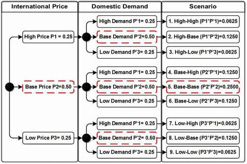
International prices and domestic demand are considered uncertain parameters with three levels: high, base, and low, with a corresponding probability for each level: 0.25, 0.50, and 0.25. The base-level represents the current values of the price and demand. While high and low levels represent the maximum increase and decrease over the 3 months planning period. These values are updated periodically at the beginning of each planning period. High and low levels are assumed 1.20 and 0.80 of the base level, as shown in Figure 5. It is assumed that the realisations of the uncertain parameters are independent to get the joint probability. Uncertain parameters were selected based on market behaviour and consistency with the HCSC literature. The above assumptions regarding scenario construction (i.e. probabilities and independency) align with the literature (Al-Othman et al. 2008; Khor, Elkamel, and Douglas 2008; Ribas, Hamacher, and Street 2010; Ribas, Leiras, and Hamacher 2011).

Figure 3. Saudi Arabia upstream crude oil SC

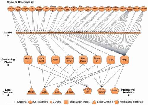
Figure 4. Saudi Arabia natural gas SC

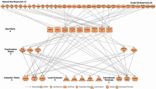
Figure 5. Scenario construction for the MOS model

5.2. Numerical results: MOS model

The length of the planning horizon in this study is three months, which is divided into a one-month planning period. The results obtained from GAMS (i.e. solved with CPLEX solver) for the case study are summarised in Table 5. To acquire more insights, the proposed stochastic model’s results are compared to the multi-objective deterministic (MOD) model proposed by (Attia, Ghaithan, and Duffuaa 2019a). The deterministic model assumes that all parameters are known and certain. The pay-off matrix listed in Tables 6 and 7 shows that the minimum total cost based on the MOS is higher than that of the MOD model the maximum revenue is lower. Therefore, in the worst case, the sustainability of MOD is better than MOS.

Table 5. MOS model statistics

Blocks of Equations	94	Single Equations	12,084
Blocks of Variables	47	Single Variables	10,880
Non-Zero Elements	65,591

Table 6. Pay-off matrix of MOS model applying lexicographic optimization

	Total Cost (M$/month)	Total Revenue (M$/month)	Depletion Rate	Sustainability (Years)
Minimizing Total Cost	13,224.94	35,215.28	0.0011825206	70.47
Maximizing Total Revenue	13,973.4	35,656.8	0.0011772191	70.79
Minimizing Depletion Rate	31,602.43	22,097.68	0.0006752586	123.41

Table 7. Pay-off matrix of MOD model applying lexicographic optimization (Attia, Ghaithan, and Duffuaa 2019a)

	Total Cost (M$/month)	Total Revenue (M$/month)	Depletion Rate	Sustainability (Years)
Minimizing Total Cost	11,487.61	36,574.97	0.001141	73.01
Maximizing Total Revenue	11,673.71	37,145.98	0.001141	73.01
Minimizing Depletion Rate	34,774.49	19,299.20	0.000578	144.20

To generate the Pareto-optima, the ranges of f2 and f3 are divided equidistantly to evaluate different resolutions, as shown in Table 8. The maximum Euclidean distance of 0.05 was used to decide whether there is a significant difference between the old and new resolutions. Then, a systematic search is applied over all possible points (i.e. 101 × 101 = 10,201 possible points). Where the coordinate of the points represents the values of (f1, f2, f3). The best resolution is 100 segments; more than this, no significance in Pareto-optima can be achieved.

Table 8. Sensitivity analysis for resolution

Resolution (segments)	Pareto Points	New Points	Maximum Euclidean distance
5	8	-	-
25	30	22	0.087
50	57	27	0.075
75	101	44	0.063
100	148	47	0.049
125	155	7	0.042
150	163	8	0.023
175	220	57	0.021
200	426	206	0.004

A set of 154 Pareto-optima is generated using the above algorithm, which shapes the trade-off between different objectives, as depicted in Figure 6. The production plan at vertex V1, Figure 6 (a), represents the worst case with a total cost of M$ 31,602.43/3 months, the revenue of M$ 22,097.68/3 months, and the sustainability of the reserves is at the maximum of 123.41 years (i.e. low depletion rate). This occurs as a result of low production levels; consequently, the shortage penalty reaches the maximum. While at vertex V2, the minimum total cost and maximum revenue can be attained but with sacrificing sustainability. Regarding the total cost, the solver produces quantities from reservoirs that compromise production, processing, and transportation costs and penalties for producing above and below the requirements.

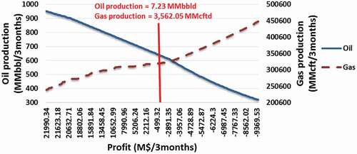
According to Figure 6, the contour plot of the Pareto-optima produced by the stochastic model behaves similarly to the one produced by the deterministic model (Attia, Ghaithan, and Duffuaa 2019a). In other words, whether using deterministic or stochastic models, the trade-off between total cost, revenue, and depletion rate is the same. The break-even analysis is shown in Figure 7, where Saudi Arabia can cover its total expenses by producing oil at 7.23 MMbbld and gas at 3,562.05 MMcftd. Not taking market uncertainty into account, the break-even points for oil and gas production are 6.96 MMbbld and 6,570.46 MMcftd, respectively. The deterministic model results in low oil production, which does not meet demand and adds to the shortage penalty. Simultaneously, gas production will increase, causing depletion and inventory levels to rise.

Finally, moving from V1 to V2, the preferred plan should be chosen by balancing the three objective functions to secure the required cash flow for sustaining Saudi Arabia’s development projects.

Figure 6. Contour plot of the Pareto-optima

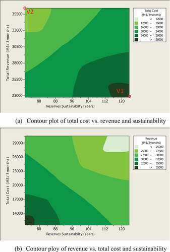
Figure 7. The relation between crude oil production and natural gas production of the MOS model

Tables 9 and 10 summarise the data of the preferred plan selected using TOPSIS (i.e. the values of the objective functions, quantity of oil production, and quantity of gas production), assuming that the weights of the objectives are equal. The MOS model provides a plan with higher cost, lower revenue, and greater sustainability due to lower levels of oil and gas productions. On the other hand, the deterministic model generates deceptive plans because it does not take into account different market scenarios (i.e. different costs and cash flows).

Table 9. Preferred plan from the MOS model

Total cost =	M$ 15,155.47/3 months	Oil production =	869.99 MMbbl/3 months
Revenue =	M$ 33,706.03/3 months		9.67 MMbbld
Profit =	M$ 18,550.56/3 months	Gas production =	275,062.99MMcft/3 months
Depletion rate =	0.00108107		3,056.26 MMcftd
Sustainability =	77.08 year

Table 10. Preferred plan from the MOD model (Attia, Ghaithan, and Duffuaa 2019a)

Total cost =	M$ 11,709.04/3 months	Oil production =	913.94 MMbbl/3 months
Revenue =	M$ 36,236.58/3 months		10.15 MMbbld
Profit =	M$ 24,527.54/3 months	Gas production =	553,251.39MMcft/3 months
Depletion rate =	0.00113568		6,147.24 MMcftd
Sustainability =	73.38 years

The solver generates quantities from reservoirs that compromise production, processing, and transportation costs, as well as the penalty for exceeding requirements (i.e. a cost that increases with production) and the penalty for falling short of requirements (i.e. a cost that decreases with production). Furthermore, there are scenarios in which prices and demand are above and below the base case, which increases the penalties (i.e. increases the expected total costs of scenario-based terms).

5.3. Sensitivity analysis: MOS model

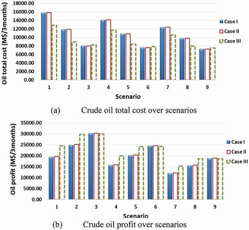
In reality, a correlation exists between product price and market demand. In this section, additional market scenarios were analysed by assigning a high probability to a high price – low demand (case II) and low price – high demand (case III). The results in Table 11 show that assigning a high probability to high demand (case III) increases crude oil production over the base-case of case I, numerical example section 4.4, and case II. Rising oil production reduces gas production and decreases the total cost due to reducing the penalty for producing below the demand. In contrast, a high probability of low prices affects the revenue and decreases the profit. As shown in Table 11, assigning a high probability to the base price and base demand yields the same plan as assigning a high probability to high price and low demand. At the same time, because of the effect of probability in the computations, the total cost and revenue are different.

Table 11. Preferred plan for the 3 cases

	Case I	Case II	Case III
Total cost (M$/3 months)	15,155.47	14,737.14	13,913.56
Revenue (M$/3 month)	33,706.03	35,629.62	33,192.13
Profit (M$/3 months)	18,550.56	20,892.48	19,278.57
Depletion rate	0.00108107	0.00108107	0.00114194
Sustainability (year)	77.08	77.08	72.98
Oil production (MMbbl/3 months)	869.99	869.99	918.98
(MMbbld)	9.67	9.67	10.21
Gas production (MMcft/3 months)	275,062.99	275,925.23	257,711.18
(MMcftd)	3,056.26	3,065.84	2,863.46

As a result of the proposed scenarios, the total cost of the crude oil decreases in the scenarios of high and base demand as a result of increasing production and decreasing the penalty for producing below demand (i.e. the shortage cost is at low levels) as shown in Figure 8(a). Similarly, the overall effect on the profit is shown in Figure 8(b). Thus, for oil, both high and base demand drives the production and profit to increase. On the contrary, a decrease in gas production leads to low profit from gas for the same scenarios.

Figure 8. Total cost and profit for crude oil based on the MOS model for the 3 cases

6. Conclusion and future research

A MOO model for tactical planning of HCSC is presented, considering uncertainties in market conditions and scenario-based optimization to develop a realistic and practical model. Furthermore, the environmental impact of HCSCs has been considered by limiting CO2 emissions. After studying three market situations (represented by nine scenarios), it is found that the highest profit is achieved for the scenario of high price – low demand conditions. In this situation, oil and gas production can be reduced. The demand during the production (shortage) can be satisfied from the outside market based on medium-term contracts to meet customer needs and, at the same time, keep enough reserves for future generations. Future research should consider the non-linearity in the HCSC (e.g. reservoir behaviour and transportation activity), utilising financial risk management to mitigate the risks associated with market uncertainty, and utilising robust optimization to find a feasible and robust solution for every scenario. Besides, it is interesting to study more different probabilities to different scenarios.

Acknowledgments

The authors would like to thank King Fahd University of Petroleum and Minerals and the Interdisciplinary Research Center of Smart Mobility and Logistics for their support in completing this work.

Disclosure statement

No potential conflict of interest was reported by the author(s).

References

- Al-Othman, W. B. E., H. M. S. Lababidi, I. M. Alatiqi, and K. Al-Shayji. 2008. “Supply Chain Optimization of Petroleum Organization under Uncertainty in Market Demands and Prices.” European Journal of Operational Research 189 (3): 822–840. doi:https://doi.org/10.1016/j.ejor.2006.06.081.
- Al-Qahtani, K., and A. Elkamel. 2010. “Robust Planning of Multisite Refinery Networks: Optimization under Uncertainty.” Computers & Chemical Engineering 34 (6): 985–995. doi:https://doi.org/10.1016/j.compchemeng.2010.02.032.
- Aseeri, A., P. Gorman, and M. J. Bagajewicz. 2004. “Financial Risk Management in Offshore Oil Infrastructure Planning and Scheduling.” Industrial & Engineering Chemistry Research 43 (12): 3063–3072. doi:https://doi.org/10.1021/ie034098c.
- Attia, A. M. 2021. “A Multi-objective Robust Optimization Model for Upstream Hydrocarbon Supply Chain.” Alexandria Engineering Journal 60 (6): 5115–5127. doi:https://doi.org/10.1016/j.aej.2021.03.046.
- Attia, A. M., A. M. Ghaithan, and S. O. Duffuaa. 2019a. “A Multi-objective Optimization Model for Tactical Planning of Upstream Oil & Gas Supply Chains.” Computers & Chemical Engineering 128: 216–227. doi:https://doi.org/10.1016/j.compchemeng.2019.06.016.
- Attia, A. M., A. M. Ghaithan, and S. O. Duffuaa. 2019b. “Data on Upstream Segment of a Hydrocarbon Supply Chain in Saudi Arabia.” Data in Brief 27: 104804. doi:https://doi.org/10.1016/j.dib.2019.104804.
- Caballero, R., E. Cerdá, M. Del Mar Muñoz, and L. Rey. 2004. “Stochastic Approach versus Multiobjective Approach for Obtaining Efficient Solutions in Stochastic Multiobjective Programming Problems.” European Journal of Operational Research 158 (3): 633–648. doi:https://doi.org/10.1016/S0377-2217(03)00371-0.
- Clemen, R. T., and T. Reilly. 2004. Making Hard Decisions with Decision Tools Suite Update Edition. 1 ed. Pacific Grove, CA: Cengage Learning.
- Conejo, A. J., M. Carrión, and J. M. Morales. 2010. Decision Making under Uncertainty in Electricity Markets. Boston, MA: Springer US.
- Dantzig, G. B. 1955. “Linear Programming under Uncertainty.” Management Science 1 (3–4): 197–206. doi:https://doi.org/10.1287/mnsc.1.3-4.197.
- Dempster, M. A. H., N. H. Pedrón, E. A. Medova, J. E. Scott, and A. Sembos. 2000. “Planning Logistics Operations in the Oil Industry.” The Journal of the Operational Research Society 51 (11): 1271–1288. doi:https://doi.org/10.1057/palgrave.jors.2601043.
- Escudero, L. F., F. J. Quintana, and J. Salmerón. 1999. “CORO, a Modeling and an Algorithmic Framework for Oil Supply, Transformation and Distribution Optimization under Uncertainty1.” European Journal of Operational Research 114 (3): 638–656. doi:https://doi.org/10.1016/S0377-2217(98)00261-6.
- Ewa, R. 2011. “Multi-Criteria Decision Making Models by Applying the Topsis Method to Crisp and Interval Data.” Multiple Criteria Decision Making/University of Economics in Katowice 6 (Mcdm): 200–230.
- Fernandes, L. J., S. Relvas, and A. P. Barbosa-Póvoa. 2015. “Petroleum Supply Chain Network Design and Tactical Planning with Demand Uncertainty.” In Operations Research and Big Data, 59–66. Springer.
- Ghaithan, A. M., A. Attia, and S. O. Duffuaa. 2017. “Multi-objective Optimization Model for a Downstream Oil and Gas Supply Chain.” Applied Mathematical Modelling 52: 689–708. doi:https://doi.org/10.1016/j.apm.2017.08.007.
- Ghatee, M., and S. M. Hashemi. 2009. “Optimal Network Design and Storage Management in Petroleum Distribution Network under Uncertainty.” Engineering Applications of Artificial Intelligence 22 (4–5): 796–807. doi:https://doi.org/10.1016/j.engappai.2009.01.003.
- Gutjahr, W. J., and A. Pichler. 2016. “Stochastic Multi-objective Optimization: A Survey on Non-scalarizing Methods.” Annals of Operations Research 236 (2): 475–499. doi:https://doi.org/10.1007/s10479-013-1369-5.
- Haugen, K. K. 1996. “A Stochastic Dynamic Programming Model for Scheduling of Offshore Petroleum Fields with Resource Uncertainty.” European Journal of Operational Research 88 (1): 88–100. doi:https://doi.org/10.1016/0377-2217(94)00192-8.
- Iakovou, E. T. 2001. “An Interactive Multiobjective Model for the Strategic Maritime Transportation of Petroleum Products: Risk Analysis and Routing.” Safety Science 39 (1–2): 19–29. doi:https://doi.org/10.1016/S0925-7535(01)00022-4.
- Jonsbråten, T. W. 1998. “Oil Field Optimization under Price Uncertainty.” Journal of the Operational Research Society 49 (8): 811–818. doi:https://doi.org/10.1057/palgrave.jors.2600562.
- Jørnsten, K. O. 1992. “Practical Combinatorial OptimizationSequencing Offshore Oil and Gas Fields under Uncertainty.” European Journal of Operational Research 58 (2): 191–201. doi:https://doi.org/10.1016/0377-2217(92)90206-O.
- Khor, C. S., A. Elkamel, and P. L. Douglas. 2008. “Stochastic Refinery Planning with Risk Management.” Petroleum Science and Technology 26 (14): 1726–1740. doi:https://doi.org/10.1080/10916460701287813.
- Li, W., C.-W. Hui, P. Li, and A.-X. Li. 2004. “Refinery Planning under Uncertainty.” Industrial & Engineering Chemistry Research 43 (21): 6742–6755. doi:https://doi.org/10.1021/ie049737d.
- Liqiang, H., and W. Guoxin, 2015. Two-stage Stochastic Model for Petroleum Supply Chain from the Perspective of Carbon Emission.
- Mavrotas, G., and K. Florios. 2013. “An Improved Version of the Augmented ε-constraint Method (AUGMECON2) for Finding the Exact Pareto Set in Multi-objective Integer Programming Problems.” Applied Mathematics and Computation 219 (18): 9652–9669. doi:https://doi.org/10.1016/j.amc.2013.03.002.
- McMurra, S. 2011. Energy to the World: The Story of Saudi ARAMCO Volume 2. 1 ed. Texas, USA: Aramco Services Company, Houston.
- MirHassani, S. A. 2008. “An Operational Planning Model for Petroleum Products Logistics under Uncertainty.” Applied Mathematics and Computation 196 (2): 744–751. doi:https://doi.org/10.1016/j.amc.2007.07.006.
- MirHassani, S. A., and R. Noori. 2011. “Implications of Capacity Expansion under Uncertainty in Oil Industry.” Journal of Petroleum Science and Engineering 77 (2): 194–199. doi:https://doi.org/10.1016/j.petrol.2011.03.009.
- Neiro, S. M. S., and J. M. Pinto. 2005. “Multiperiod Optimization for Production Planning of Petroleum Refineries.” Chemical Engineering Communications 192 (1): 62–88. doi:https://doi.org/10.1080/00986440590473155.
- Oliveira, F., and S. Hamacher. 2012. “Optimization of the Petroleum Product Supply Chain under Uncertainty: A Case Study in Northern Brazil.” Industrial & Engineering Chemistry Research 51 (11): 4279–4287. doi:https://doi.org/10.1021/ie2013339.
- Ribas, G., A. Leiras, and S. Hamacher. 2011. “Tactical Planning of the Oil Supply Chain: Optimization under Uncertainty.” PRÉ-ANAIS XLIIISBPO, 2258–2269.
- Ribas, G. P., S. Hamacher, and A. Street. 2010. “Optimization under Uncertainty of the Integrated Oil Supply Chain Using Stochastic and Robust Programming.” International Transactions in Operational Research 17 (6): 777–796. doi:https://doi.org/10.1111/j.1475-3995.2009.00756.x.
- Sahebi, H., S. Nickel, and J. Ashayeri. 2014. “Strategic and Tactical Mathematical Programming Models within the Crude Oil Supply Chain context—A Review.” Computers & Chemical Engineering 68: 56–77. doi:https://doi.org/10.1016/j.compchemeng.2014.05.008.
- Stewart, M., and K. E. Arnold. 2007. Surface Production Operations, Volume 1, Third Edition: Design of Oil Handling Systems and Facilities. 3 ed. Amsterdam; Boston: Houston, Tex.? Gulf Professional Publishing.
- Tarhan, B., I. E. Grossmann, and V. Goel. 2009. “Stochastic Programming Approach for the Planning of Offshore Oil or Gas Field Infrastructure under Decision-Dependent Uncertainty.” Industrial & Engineering Chemistry Research 48 (6): 3078–3097. doi:https://doi.org/10.1021/ie8013549.
- Tong, K., Y. Feng, and G. Rong. 2012. “Planning under Demand and Yield Uncertainties in an Oil Supply Chain.” Industrial & Engineering Chemistry Research 51 (2): 814–834. doi:https://doi.org/10.1021/ie200194w.
- Tzeng, G. H., and J. J. Huang. 2011. Multiple Attribute Decision Making: Methods and Applications. Multiple Attribute Decision Making: Methods and Applications. CRC Press.
- Yang, J., H. Gu, and G. Rong. 2010. “Supply Chain Optimization for Refinery with Considerations of Operation Mode Changeover and Yield Fluctuations.” Industrial & Engineering Chemistry Research 49 (1): 276–287. doi:https://doi.org/10.1021/ie900968x.