Fully parallel, OpenGL-based computation of obstructed area-to-area view factors

Abstract

We present a fully parallelized, high-performance, OpenGL-based approach to compute obstructed area-to-area (A2A) view factors for radiative heat transfer. The A2A view factors are computed from the defining surface integral by Gaussian quadrature. The values of the integrand, i.e. the point-to-area view factors, are computed using an OpenGL-based hemicube (HC) method to efficiently solve the obstruction problem by exploiting the hardware-accelerated visibility testing on modern graphics cards. The final steps to maximize hardware usage are rendering the HC and performing the numerical quadrature in parallel such that data transfer times are completely shadowed by computations. To demonstrate the power of our approach we compute the A2A view factor matrices for a warehouse equipped with ceramic infrared heaters and a test cabin conforming to EN 442 containing a section of a panel radiator. To judge the quality of the results we measure the deviation from unity of the area-weighted column sums of the view factor matrix and the error in radiant flux balance. Compared to a previous, ray-tracing-based implementation, we gain three orders of magnitude in speed in the view factor computation. Conservation of radiant flux is also substantially improved.

Keywords:

• obstructed view factors
• radiative heat transfer
• building simulations
• task parallelism
• hemicube
• OpenGL

1. Introduction

The accurate and fast computation of obstructed view factors is one of the long-standing issues in radiative heat transfer (RHT). View factors represent the fraction of radiant energy emitted by a given surface that is intercepted by another one. They are at the heart of any building energy simulation, e.g. of heating, ventilation, and air-conditioning systems (Kim, Kato, and Murakami 2001), of thermal comfort prediction (Tanabe et al. 2002; Lube et al. 2008) or of the influence of incident solar radiation (Jones, Greenberg, and Pratt 2012). Further domains of application of equal importance are the design and simulation of experiments in high energy density physics (MacFarlane 2003), multi-physics flow and solidification (Swaminarayan and Turner 2007) or nuclear reactor core design (Bopche and Sridharan 2009).

The main problem in computing view factors is to deal with occlusion effects, i.e. blocking of radiation due to geometry, efficiently.

In contrast to other fields of application detailed building simulations require an accurate calculation of area-to-area (A2A) view factors between surfaces which often are subject to (partial) occlusion. In computer graphics (CG) view factors arise in the calculation of indirect lighting, also called global illumination (GI), and are an integral part of photo-realistic image synthesis (Cohen, Wallace, and Hanrahan 1993). From an algorithmic point of view the key development was the introduction of hierarchical radiosity (HR) (Hanrahan, Salzman, and Aupperle 1991). Using ideas developed for many-body simulations in physics, especially for the molecular dynamics of large molecules, HR reduces algorithmic complexity from quadratic to essentially linear in the number of surface elements. Over the years HR was substantially improved, yet the main boost in performance came from moving further computations to the graphics card (Lum, Ma, and Max 2002; Coombe, Harris, and Lastra 2004; Lum, Ma, and Max 2005). In HR the occlusion problem is mostly solved by adaptive mesh refinement. Then, instead of A2A view factors which are subject to (partial) occlusion, rather a large number of unobstructed point-to-area (P2A) or point-to-point (P2P) view factors are needed. However, in HR the values and the number of the view factors become solution-dependent because the mesh refinement is driven by the error in the particular solution which is less useful for building simulations where the goal is to determine RHT with respect to the material properties of the surfaces in a building. Furthermore, if derived quantities like the Gebhart factors are to be computed or if the radiative transfer problem is solved by the network method, A2A view factors need to be known explicitly.

Although RHT and GI are described by the same equation (Goral et al. 1984) the requirements on the solution are quite different. In case of GI, which is one of the major topics in CG, the goal is to obtain a solution which looks “correct” but is not in the strict mathematical sense. In many computer games, a GI solution is needed only from the point of view of the player (so-called first-person perspective) which allows for further tweaks to reduce the amount of necessary computational resources (Smits, Arvo, and Salesin 1992) to achieve interactive GI computations. One technical solution to the needs of CG was to create dedicated graphics processing units (GPU) with the fundamental CG algorithms implemented in silico, i.e. to provide hardware acceleration. Especially depth testing, which is a precursor to any occlusion query, is done with full hardware acceleration and thus is very attractive as aid in engineering-related tasks. A convenient tool for graphics-related computations is OpenGL which provides a set of tailor-made functions for rendering the lighting of a three-dimensional scene with full hardware acceleration.

1.1. Previous work

Depending on the community, different solutions to the problem of a fast and accurate view factor computation have been conceived. Originally an RHT problem, the determination of view factors became a popular topic in the CG community in the 1980s and 1990s. When implemented in OpenGL such that rendering takes place on a graphics card, the hemicube (HC) algorithm (Cohen and Greenberg 1985) provides an efficient tool to compute obstructed P2A view factors. Combined with numerical quadrature this provides an accurate way of computing obstructed A2A view factors.

For validation purposes of GI algorithms, the problem of the A2A view factor between two arbitrary, unobstructed polygons has been solved in closed form (Schröder and Hanrahan 1993). They involve a lot of calls to special functions which makes them less attractive for on-the-fly computations on GPUs due to their limited performance in special function evaluations. Nowadays in CG, view factors are usually computed on the GPU (Lum, Ma, and Max 2002; Coombe, Harris, and Lastra 2004; Lum, Ma, and Max 2005).

In RHT view factors often are obtained from large collections of pre-computed configurations (e.g. Howell 1982). Precomputing view factors is discussed in the standard textbooks (e.g. Modest 2003 or Faghri, Zhang, and Howell 2010). The definition of view factors leads to a nested integration over two areas so that a computation by numerical quadrature may become prohibitively costly in case of an inefficient implementation.

Without obstruction the double area integral (2AI) can be converted into two nested contour integrals (2CI) using Stokes’ theorem. The attempts to control accuracy by adaptive quadrature are described in Walton (2002) and an open-source implementation is available (Walton and Pye 2011). A recent attempt based on the 2AI (Dobrowolski de Carvalho Augusto, Giacomet, and Mendes 2007) is entirely CPU based as well. There are also discussions of the particular problems which arise from curved surfaces (Bao and Peng 1994). For geometries of particular importance special solutions exist, for instance in nuclear reactor design (Bopche and Sridharan 2009; Feng and Han 2012). Combined with local mesh refinement, Francisco et al. (2013) use Stokes’ theorem for obstructed view factors. However, this approach does not discuss any hardware acceleration either. The main shortcoming of non-CG approaches to the computation of obstructed view factors is that they have to re-implement many of the algorithms for visibility testing which are readily available in hardware-accelerated form on the GPU and for which OpenGL provides a usable and hardware-independent programming interface. Its use gets further simplified by the C++-wrapper classes provided by the QT library.

The key to overcome the occlusion problem while increasing performance is to take advantage of hardware-accelerated visibility testing by employing the HC algorithm in its OpenGL-based form (Cohen and Greenberg 1985; Lum, Ma, and Max 2002). While aliasing has been an issue in the past (Max 1995), on nowadays GPUs, the resolution of the HC can be chosen almost arbitrarily fine so that for practical purposes P2A view factors can be considered as exact.

This short review is restricted to methods working with view factors for diffusively emitting surfaces which enclose non-participating media. There are a number of other ways for computing RHT, for instance the discrete ordinate method, which is still a matter of investigation and improvement (see e.g. Koch and Becker 2004 or Mishra, Roy, and Misra 2006) and is also available in some commercial tools. In addition, building performance simulation programs originally did not work with such detailed methods for RHT. In order to generate predictions for the energy consumption for heating periods or years, simplified methods were applied, like balance equations without view factors or heat transfer coefficients (e.g. Elsner, Fischer, and Huhn 1993, Sec. 5.7).

1.2. Our approach

It is the aim of this paper to transfer some of the high-performance solutions of CG for view factor computation to the field of RHT. Compared to previous implementations (Perschk 2000; Francisco et al. 2013) we gain a striking speedup of three orders of magnitude.

The view factors between all surfaces in a building, or more abstract: scene, can be arranged in a matrix which, depending on the degree of obstruction, can be anything from sparse to dense. Each view factor between two surfaces, each of finite size, is computed by Gaussian quadrature (Stroud 1971) of the 2AI. At each quadrature point we have to render one HC which gives us the point-to-texel (P2Tx) view factors belonging to the projections of the visible parts of the other surfaces onto the HC. The P2A view factors are computed by summing up the P2Tx view factors. In contrast to the approaches mentioned above, which monitor the error in the energy transport between individual pairs of surfaces, the HC method gives us an entire row of the view factor matrix at once making error control more difficult.

The main observation concerning parallelization is that the calculation of an individual row of the A2A view factor matrix is completely independent of all the other rows. Furthermore, the individual P2A view factors needed to compute the A2A view factors by numerical quadrature are also independent of each other. Hence, the overall problem of computing the A2A view factor matrix is highly parallel on several levels and thus can easily be distributed over several compute nodes. To be more specific, communication between different compute nodes is realized with the networking module of the QT library (Blanchette and Summerfield 2008). On each compute node the rendering of the HC on the GPU and the summation of the P2Tx view factors on the CPU is parallelized according to the producer–consumer model (Wilson and Lu 1996). The implementation is based on the multithreading module of the QT library. The GPU produces rendered HCs, i.e. large arrays of P2Tx view factors, and the CPU consumes them to form the P2A view factors which ultimately get condensed into the A2A view factors of one row. Similar to our approach OpenGL has been successfully employed for the accurate computation of direct solar radiation on building surfaces of complex shape at high speeds (Jones, Greenberg, and Pratt 2012).

The paper is organized as follows. In Section 2, we briefly repeat the properties of view factors and recall how to compute P2A view factors from the OpenGL-based HC. Section 3 discusses the details of the parallelization of the overall computation and the resulting software design. The influence of the method's parameters and the efficiency of the parallelization are discussed in Section 4 using two toy scenes, the unit cube and two concentric cubes, and two real-life test cases. The conclusions are drawn and an outlook is given in Section 5.

2. View factors

View factors are mere geometric quantities. They are defined as the fraction of the energy emitted from a surface ${\mathbf{A}}_{\mathbf{i}}$ by radiation which directly reaches another surface ${\mathbf{A}}_{\mathbf{j}}$. We denote surfaces including their orientation (expressed by their normal vectors) by bold-face, capital letters while regular capital letters only denote the area of a surface. A detailed discussion of their derivation and computation for numerous special cases in the absence of occlusion is given in many books about RHT (e.g. Modest 2003). We just recall the necessary facts which are important for a discussion of a parallel implementation and error estimation.

2.1. Differential P2P view factors

The differential view factor $\mathrm{d}{F}_{\mathrm{d}{A}_i\to \mathrm{d}{A}_j}$ between two differential surfaces $\mathrm{d}{\mathbf{A}}_{\mathbf{i}}$ and $\mathrm{d}{\mathbf{A}}_{\mathbf{j}}$ follows from the differential energy flux $I({\mathbf{x}}_{\mathbf{i}}\mathbf{)}\mathrm{d}{\mathbf{A}}_{\mathbf{i}}\cos {\theta }_{\mathbf{i}}\mathrm{d}\mathbf{\Omega }$ at position ${\mathbf{x}}_{\mathbf{i}}$ on ${\mathbf{A}}_{\mathbf{i}}$ with radiation intensity $I({\mathbf{x}}_{\mathbf{i}}\mathbf{)}$ into the differential solid angle d Ω forming the angle θ_i with the surface normal. The area of the effective cross section of the surface $\mathrm{d}{\mathbf{A}}_{\mathbf{j}}$ at distance $r=|{\mathbf{x}}_{\mathbf{j}}\mathbf{-}{\mathbf{x}}_{\mathbf{i}}\mathbf{|}$, visible from $\mathrm{d}{\mathbf{A}}_{\mathbf{i}}$, is $\mathrm{d}{A}_j\cos {\theta }_j$. The solid angle subtended by $\mathrm{d}{\mathbf{A}}_{\mathbf{j}}$ when viewed from $\mathrm{d}{\mathbf{A}}_{\mathbf{i}}$ is $\mathrm{d}\mathrm{\Omega }=\mathrm{d}{A}_j\cos {\theta }_j/r^2$ and the energy flux between the two differential surfaces is $I({\mathbf{x}}_{\mathbf{i}}\mathbf{)}\mathrm{d}{\mathbf{A}}_{\mathbf{i}}\cos {\theta }_{\mathbf{i}}\cos {\theta }_{\mathbf{j}}\mathrm{d}{\mathbf{A}}_{\mathbf{j}}\mathbf{/}{\mathbf{r}}^{\mathbf{2}}$. Dividing by the total amount of energy $\pi I({\mathbf{x}}_{\mathbf{i}}\mathbf{)}\mathrm{d}{\mathbf{A}}_{\mathbf{i}}$ diffusively emitted by $\mathrm{d}{\mathbf{A}}_{\mathbf{i}}$ gives the differential view factor

$\mathrm{d}{F}_{\mathrm{d}{A}_i\to \mathrm{d}{A}_j}=\frac{\cos {\theta }_i\cos {\theta }_j}{\pi r^2}\mathrm{d}{A}_j.$

Since the indexes i and j are arbitrary they can be swapped which leads to the reciprocity relation

$\mathrm{d}{A}_i\mathrm{d}{F}_{\mathrm{d}{A}_i\to \mathrm{d}{A}_j}=\mathrm{d}{A}_j\mathrm{d}{F}_{\mathrm{d}{A}_j\to \mathrm{d}{A}_i}.$

2.2. Differential P2A view factors

2.2.1. General case

Integrating the P2P view factor (1) over a distant area ${\mathbf{A}}_{\mathbf{j}}$ of finite size yields an expression for the relative amount of energy radiatively transferred from $\mathrm{d}{\mathbf{A}}_{\mathbf{i}}$ to ${\mathbf{A}}_{\mathbf{j}}$, i.e. the P2A view factor

$\mathrm{d}{F}_{\mathrm{d}{A}_i\to A_j}={\int }_{A_j}\frac{\cos {\theta }_i({\mathbf{x}}_{\mathbf{i}}\mathbf{,}{\mathbf{x}}_{\mathbf{j}}\mathbf{)}\cos {\theta }_{\mathbf{j}}\mathbf{(}{\mathbf{x}}_{\mathbf{i}}\mathbf{,}{\mathbf{x}}_{\mathbf{j}}\mathbf{)}}{\pi |{\mathbf{x}}_{\mathbf{i}}\mathbf{-}{\mathbf{x}}_{\mathbf{j}}{\mathbf{|}}^{\mathbf{2}}}\mathrm{d}{A}_j.$

The choice of coordinates is given in Figure 1. If ${\mathbf{A}}_{\mathbf{j}}$ is (partially) obstructed integration has to be carried out only over the visible part ${\tilde{\mathbf{A}}}_j$. The angles θ_i and θ_j with respect to the surface normals depend not only on their respective normal, but due to the vector $\mathbf{r}\mathbf{=}{\mathbf{x}}_{\mathbf{j}}\mathbf{-}{\mathbf{x}}_{\mathbf{i}}$ on positions on both surfaces. Similar to the differential P2P view factor, Equation (3) describes the relative amount of energy flux from a differential area to an area of finite size. The reverse situation, the energy transfer from a surface of finite size to an infinitesimally small one, can be obtained by swapping the indexes i and j.

Figure 1. Geometry of RHT between differential surfaces leading to the definition of differential view factors.

2.2.2. Closed expressions for polygons

If both surfaces are planar, unobstructed polygons, especially the distant ${\mathbf{A}}_{\mathbf{j}}$, the P2A and the A2A view factor can be computed from closed expressions which are derived from the 2CI (Schröder and Hanrahan 1993).

The point-to-polygon view factors for any point $\mathbf{p}\in \mathrm{d}{\mathbf{A}}_{\mathbf{i}}$ follow from the angles formed by the normal ${\mathbf{n}}_{\mathbf{i}}$ of $\mathrm{d}{\mathbf{A}}_{\mathbf{i}}$ and the vectors ${\mathbf{v}}_{\mathbf{k}}\mathbf{=}{\mathbf{q}}_{\mathbf{k}}\mathbf{-}\mathbf{p}$, which point to the n corners ${\mathbf{q}}_{\mathbf{k}}$ of the polygon ${\mathbf{A}}_{\mathbf{j}}$ (numbered in clockwise order with respect to ${\mathbf{n}}_{\mathbf{j}}$ which points from A_j to $\mathbf{p}$, cf. Figure 2). They can be computed from a sum of inner products (Lum, Ma, and Max 2005)

$F_{\mathrm{d}{A}_i\to A_j}=\frac{1}{2\pi }\sum _{k=1}^n{\mathbf{n}}_{\mathbf{i}}\cdot {\mathbf{G}}_{\mathbf{k}}\mathbf{.}$

Figure 2. Choice of coordinate system for the computation of P2A view factors and projection of a distant surface A_j onto the HC. Summation of the point-to-pixel view factors belonging to the shaded pixels gives the P2A view factor of A_j. The projection of all distant surfaces A_j is done by rendering them with OpenGL on the graphics card. The camera is located at p and points into the z-direction.

The vector ${\mathbf{G}}_{\mathbf{k}}$ is defined as

${\mathbf{G}}_{\mathbf{k}}\mathbf{:=}\frac{{\gamma }_{\mathbf{k}}}{\mathbf{|}{\mathbf{g}}_{\mathbf{k}}\mathbf{|}}{\mathbf{g}}_{\mathbf{k}}\mathbf{.}$

Its length corresponds to the angle γ_k between two successive vectors ${\mathbf{v}}_{\mathbf{k}\mathbf{+}\mathbf{1}}$ and ${\mathbf{v}}_{\mathbf{k}}$ from $\mathbf{p}$ to the corners ${\mathbf{q}}_{\mathbf{k}}$. The ratio of their outer product

${\mathbf{g}}_{\mathbf{k}}\mathbf{:=}{\mathbf{v}}_{\mathbf{k}\mathbf{+}\mathbf{1}}\times {\mathbf{v}}_{\mathbf{k}}$

and inner product gives

$\tan ({\gamma }_k)=\frac{{\mathbf{v}}_{\mathbf{k}\mathbf{+}\mathbf{1}}\times {\mathbf{v}}_{\mathbf{k}}}{{\mathbf{v}}_{\mathbf{k}\mathbf{+}\mathbf{1}}\cdot {\mathbf{v}}_{\mathbf{k}}}.$

The reason for using $\tan ({\gamma }_k)$ and not $\sin ({\gamma }_k)$ or $\cos ({\gamma }_k)$ is that its inverse is less susceptible to round-off errors.

2.3. OpenGL-based HC method

The basis for an accurate numerical computation of obstructed A2A view factors are precise values for obstructed P2A view factors for which we use Equation 3. To simplify its evaluation we exploit Gauss’ theorem which states that for the computation of a flux through some surface only its effective cross-section matters, i.e. its projection onto the plane orthogonal to the direction of the flux. Hence, in order to compute the flux from a point $\mathbf{x}$ to the surface ${\mathbf{A}}_{\mathbf{j}}\mathbf{,}$ the only quantity of interest is the solid angle subtended by ${\mathbf{A}}_{\mathbf{j}}$ when viewed from $\mathbf{x}$.

The point $\mathbf{p}\in \mathrm{d}{\mathbf{A}}_{\mathbf{i}}$ can be used as origin of a local coordinate system with the z-axis pointing into the same direction as the surface normal (Figure 2). This defines the visible HC around the point $\mathbf{p}$. By projecting all distant surfaces onto an HC we can figure out which other surfaces are visible and how large their visible part actually is. The resolution of the HC is determined by its number of texels per coordinate direction N_tx. The texel diameter is denoted as H, which is proportional to 1/N_tx and is distinct from the diameter h of an element of the surface mesh.

For the OpenGL-based implementation the HC surface is subdivided into a regular grid. Each rendering with OpenGL gives us the projection of the scene onto one of the HC faces and therefore we have to draw the scene five times from each point of view. Once in the positive z-direction to project onto the top and then into the ±x- and ±y-directions for the four lateral faces. A sample HC rendering is shown in the framebuffer object (FBO) in Figure 4.

To identify the projected surfaces they are numbered consecutively and their indexes are converted by bit-shift operations from 32-bit integer into 8-bit blocks which then are used as red, green, blue and α components of a uniquely assigned colour. This allows for $2^{32}\approx 4\times {10}^9$ individual surface elements in a scene. Each texel on the HC represents a particular P2Tx view factor which is computed from Equation (4) only once at the beginning and the texel's colour identifies the surface projected to it.

The P2A view factor of ${\mathbf{A}}_{\mathbf{j}}$ is simply the sum of the P2A view factors of the individual texels covered by $A_j^{\perp }$

$\mathrm{d}{F}_{\mathrm{d}{A}_i\to A_j}^H=\sum _{(x,y)\in A_{\overline{j}}}\mathrm{\Delta }{F}_{xy}+\sum _{(y,z)\in A_j^{\perp }}\mathrm{\Delta }{F}_{yz}+\sum _{(x,z)\in A_j^{\perp }}\mathrm{\Delta }{F}_{xz},$

where Δ F_xy is a P2Tx view factor on the top of the HC, Δ F_yz is a P2Tx view factor on one of the faces parallel to the yz-plane and Δ F_xz corresponds to a P2Tx view factor on one of the faces parallel to the xz-plane (cf. Figure 2).

2.4. A2A view factors by numerical quadrature

The obstructed A2A view factors are computed from their definition $F_{A_i\to {\tilde{A}}_j}:=\frac{1}{A_i}{\int }_{A_i}{\int }_{{\tilde{A}}_j}\frac{\cos {\theta }_i\cos {\theta }_j}{\pi |{\mathbf{x}}_{\mathbf{i}}\mathbf{-}{\mathbf{x}}_{\mathbf{j}}{\mathbf{|}}^{\mathbf{2}}}\mathrm{d}{\tilde{A}}_j\mathrm{d}{A}_i,$ but with integration over the visible part ${\tilde{A}}_j$ of A_j. Strictly speaking, ${\tilde{A}}_j$ is a function of ${\mathbf{x}}_{\mathbf{i}}$. This is automatically resolved by the HC method. In general, these integrals cannot be solved in closed form. Rather, we have to compute their values by means of numerical quadrature, also called cubature for multiple integrals. Let $\mathrm{d}{F}_{\mathrm{d}{A}_i\to {\tilde{A}}_j}^H({\mathbf{x}}_{\mathbf{i}\mathbf{,}\alpha }\mathbf{)}$ denote the P2A view factor from Equation (8) at the quadrature point ${\mathbf{x}}_{\mathbf{i}\mathbf{,}\alpha }\in {\mathbf{A}}_{\mathbf{i}}$ and w_α the corresponding quadrature weight. Then, the numerical expression for the A2A view factor is

$F_{A_i\to {\tilde{A}}_j}^h=\sum _{\alpha }{w}_{\alpha }\mathrm{d}{F}_{\mathrm{d}{A}_i\to {\tilde{A}}_j}^H({\mathbf{x}}_{\mathbf{i}\mathbf{,}\alpha }\mathbf{)}\mathbf{.}$

The superscript h denotes the diameter of the circle enclosing the triangle we integrate over and is a measure for its size (cf. Figure 3). It is also synonymously used as a measure for the size of the elements of the surface mesh. It is common to tabulate quadrature points ${\mathbf{x}}_{\alpha }$ and weights ${\omega }_{\alpha }$ with respect to a reference element ˆ K, e.g. the triangle with corners (0,0), (1,0), (0,1) or the square with corners (−1,−1), (1,−1), (1,1), (−1,1). Therefore, a surface element K of arbitrary shape has to be mapped to the reference element ˆ K by an affine transformation $J:\hat{\mathbf{x}}\in \hat{K}\to \mathbf{x}\in \mathbf{K}$ before the quadrature of some function $f:K\to \mathbb{R}$ can be performed:

${\int }_{K}f(\mathbf{x}\mathbf{)}\mathrm{d}\mathbf{K}\mathbf{=}{\int }_{\stackrel{\mathbf{ˆ}}{\mathbf{K}}}\mathbf{f}\mathbf{(}\mathbf{J}\stackrel{\mathbf{ˆ}}{\mathbf{x}}\mathbf{)}\mathbf{|}det{\mathbf{J}}^{\prime }\mathbf{(}\stackrel{\mathbf{ˆ}}{\mathbf{x}}\mathbf{)}\mathbf{|}\mathrm{d}\stackrel{\mathbf{ˆ}}{\mathbf{K}}\mathbf{.}$

Figure 3. Quadrature subdivision for the computation of obstructed A2A view factors. Details see text.

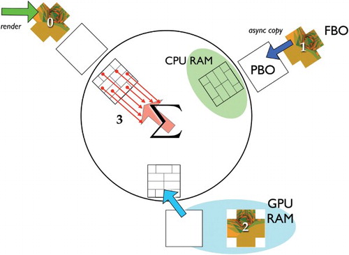
Figure 4. (Colour online) Pipelining and parallelization of the HC rendering and the summation of the P2Tx view factors. The HC gets rendered into a framebuffer object (FBO), step (0), while the content of another FBO is copied into a pixel buffer object (PBO), step (1). At the same time data from another PBO is copied from the GPU to the CPU side of the PCI-express bus by means of a direct memory access transfer, step (2). Parallel to these buffer operations the contents of a CPU-side copy of a PBO are summed up to get the P2A view factors, step (3). The image in the FBO is a sample image of a rendered HC. Each stage of the pipeline has its own set of FBO, PBO and CPU-side PBO mirror. The tiles in the latter indicate how different parts of the image of the HC are distributed among several threads for computing the P2A from the P2Tx view factors.

In our case f represents the P2A view factor function and K is A_i. For a planar triangle the Jacobian determinant det J′ is constant, equals the size of the area and cancels the factor 1/A_i from the definition of the A2A view factor. Prior to integration we split quadrilaterals into triangles and the final value of the integral is obtained from summing over these triangles. The reason for this is that area integration is best understood for simplices; in case of a two-dimensional manifold like a surface mesh, these are triangles, and thus for triangles, we have the largest choice of quadrature rules. For rendering it is not necessary to split quadrilateral elements. Further details about calculating multiple integrals by numerical quadrature can be found in Stroud (1971).

Since integration always involves a mapping from the physical element to the reference element, we do not have to design special quadrature rules for non-planar polygons. For curved elements the work is better invested in the setup of the nonlinear transformation of an element onto the planar reference elements. This is also valid for quadrilaterals. A good source for a discussion of this topic is the set of tutorial programs of the deal.II library (Bangerth, Hartmann, and Kanschat 2007) and the documentation of the different Mapping classes.

Since visibility between two surfaces is a highly discontinuous function we only use low-order quadrature rules and resolve occlusion effects by multiple regular subdivisions of the surface elements, i.e. on each subdivision a triangle gets recursively split into four new triangles by connecting the midpoints of the old triangle's edges (cf. Figure 3). On each subtriangle $\mathbf{T}\subset {\mathbf{A}}_{\mathbf{i}}$ we apply the quadrature rule and sum over all subsurfaces:

$F_{A_i\to {\tilde{A}}_j}^h=\sum _{T\subset A_i}\sum _{\alpha }{w}_{\alpha }\mathrm{d}{F}_{\mathrm{d}{A}_i\to {\tilde{A}}_j}^H({\mathbf{x}}_{\mathbf{i}\mathbf{,}\alpha }^{\mathbf{(}\mathbf{T}\mathbf{)}}\mathbf{)}\mathbf{.}$

A quadrature point within a subtriangle $\mathbf{T}$ is denoted as ${\mathbf{x}}_{\mathbf{i}\mathbf{,}\alpha }^{\mathbf{(}\mathbf{T}\mathbf{)}}$. As quadrature rule we use the 3-point Gauss–Legendre quadrature for planar triangles. The barycentric coordinates of the quadrature points ${\mathbf{x}}_{\mathbf{i}\mathbf{,}\alpha }^{\mathbf{(}\mathbf{T}\mathbf{)}}$ and its quadrature weights w_α are given in Table 1 (Hammer, Marlowe, and Stroud 1956). Gauss–Legendre rules belong to the class of interpolating quadrature rules, i.e. quadrature points and weights are chosen such that polynomials up to a certain degree are integrated exactly. The number of subdivision steps is denoted as n_s, yielding $4^{n_s}$ triangles.

Table 1.  Barycentric coordinates (p_x, p_y, p_z) and weights w_α of the 3-point Gauss–Legendre quadrature on a triangle.

px	py	pz	wα
2/3	1/6	1/6	1/6
1/6	2/3	1/6	1/6
1/6	1/6	2/3	1/6

Note: Weights are normalized such that their sum equals the area of the reference triangle with corners (0,0), (1,0), (0,1).

3. Software design

The basis of our software is the QT library because of its platform independence and its OpenGL module. The latter provides a large set of C++-wrapper classes which tremendously simplify the OpenGL handling. The off-loading of the OpenGL rendering into a separate thread is based on Hanke (2009). The implementation of the HC method in OpenGL is based on the RRV package (Dudka 2007).

To achieve a performance close to the theoretical limits of the hardware it is important to observe that for different quadrature points the following major steps can all be done in parallel:

• (1) rendering the HC on the GPU,

• (2) transferring data from the GPU to the CPU,

• (3) summation of the P2Tx into the P2A view factors and their subsequent condensation into the A2A view factors on the CPU.

The parallel execution of these steps is the crucial point for accelerating the computational time by three orders of magnitude. The parallel implementation hinges on the pipelining scheme illustrated in Figure 4.

To provide a better understanding of the parallelization scheme we describe it in more detail in the following. The program consists of two parts which run in separate threads. The main thread hosts the graphical user interface (GUI) and the other thread manages the computation of the view factors. The former is called the GUI thread and the latter the worker thread. This avoids a blocking of the GUI by compute-intensive tasks. Within the worker thread we need a further level of task parallelism so that rendering the HC and the evaluation of Equations (8) and (11) are done in a concurrent manner according to the producer–consumer model (Wilson and Lu 1996). We have to start one thread for the actual OpenGL rendering (producer) and another one for the management of the summation of the P2Tx view factors (consumer). Synchronization is implemented using semaphores. The complete process of rendering, data transfers and evaluating Equation (8) is realized as a three-staged pipeline consisting of four steps (cf. Figure 4). In order to avoid sharing the OpenGL context between different threads, the data transfers are all done from within the producer thread. Modern GPUs are equipped with a dedicated memory controller such that they bypass the CPU when transferring data, i.e. they are able to perform so-called DMA (direct memory access) transfers. To do this, the data on the GPU side must be stored in pixel buffer objects (PBO). To use this hardware-assisted parallelization, the data transfer from the GPU to the main memory must take place in two stages. In the first stage, the HC is rendered off screen into an FBO, step 0 in Figure 4, which then, in the second stage, gets copied into a PBO, step 1 in Figure 4. In the third stage of the pipeline, all major steps are executed in parallel: as soon as the FBO-to-PBO transfer is done the GPU is ready to render the HC with respect to the next quadrature point. This is step 0 again. Simultaneously, step 2 can take place: the transfer of the contents of another PBO across the PCI-express (PCIe) bus into the main memory of the computer. While the data transfers are under way the consumer thread starts further threads in order to execute the summation of the P2Tx view factors in parallel for which the HC gets subdivided into several tiles as indicated in Figure 4. Usually as many threads are employed as there are physical cores in the CPU. This is indicated by the bunch of arrows pointing at Σ in Figure 4 and forms step 3. Each stage of the pipeline has its own set of FBO, PBO and CPU-side PBO mirror, i.e. altogether we have to reserve memory for six HC on the GPU and three on the CPU side. Eventually, the P2A view factors are added to a buffer for the A2A view factors which gets copied into the view factor matrix only after all $4^{n_s}$ quadrature points of one surface element have been processed.

4. Results

All tests are performed on the machines listed in Table 2. We will discuss three aspects of numerically computing obstructed A2A view factors. Accuracy is assessed in Section 4.3. The efficiency of the implementation is demonstrated in Section 4.4 and the quality of the radiant flux balance is investigated in Section 4.5.

Table 2.  Computers used in tests.

Manufacturer	Name	CPU (Intel)	Cores (+HT)	GPU (NVidia)	OS (Compiler)
Asus	k53	Core i7-2630QM	4 (8)	GeForce GT540m	W7HP (mingw-g++-4.4)
					opensuse 12.1 (g++-4.6)
					Ubuntu 11.10 (g++-4.6)
Dell	c3	Xeon E5520	4	Tesla C2070	Ubuntu 10.04 (g++-4.4)
Dell	c4	2 Xeon X5650	12 (24)	GeForce GTX460	Ubuntu 10.04 (g++-4.4)
Dell	c5	2 Xeon X5675	12 (24)	Tesla C2070	Ubuntu 10.04 (g++-4.4)
Dell	c6	2 Xeon X5675	12 (24)	Tesla C2070	Ubuntu 12.04 (g++-4.6)
Apple	retina	Core i7-3820QM	4 (8)	GeForce GT 650M	Mac OS 10.8.5 (apple-g++-4.7)

Note: All operating systems were 64 bit.

4.1. Test cases

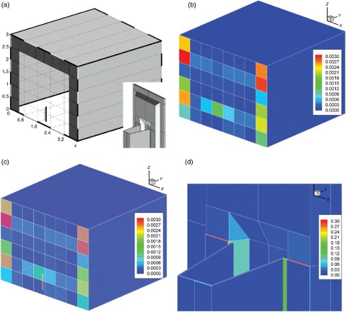
In general, it is difficult to come up with a model scene for which the values of obstructed A2A view factors can be calculated exactly by means of an analytic expression in order to have a reference for the numerically obtained ones. We test the accuracy of the view factor computation on the unit cube and the “concentric cube” scene of Francisco et al. (2013). The latter scene provides a simultaneous test of obstructed and unobstructed configurations of pairs of surface elements. In this particular setup the inner cube is of size $1\mathrm{m}\times 1\mathrm{m}\times 1\mathrm{m}$ and the outer one is $3\mathrm{m}\times 3\mathrm{m}\times 3\mathrm{m}$ (Figure 5(a)). For the concentric cubes we can compute exact values even for some of the obstructed view factors ($F_{1\to \mathrm{II}}$ and $F_{\mathrm{II}\to 1}$).

Figure 5. (a) Geometry of the concentric cubes. Dimensions are 1 m×1 m×1 m and 3 m×3 m×3 m, respectively. Face numbering is such that the sum of the indexes of opposite faces equals 7. For the inner cube we use roman numbers. (b)Mutually different A2A view factors for this scene. The view factors (F_1→II and F_II→1) are obstructed.

The unit cube is the test bed for the convergence properties of the HC in the absence of any occlusion effects. There are only two mutually different A2A view factors: $F_{\mathrm{ops}}=0.199825$ for faces opposite to each other and $F_{\mathrm{adj}}=0.200044$ for faces sharing an edge.

To assess the performance of our implementation on realistic geometries similar to Jones, Greenberg, and Pratt (2012), we use two scenes from our current research. Both cases have in common that the sizes of the surface elements differ by several orders of magnitude and that their surface elements often have large aspect ratios.

The first test case is a test cabin conforming to EN 442 (DIN EN 442-2 2003) containing a section of a panel radiator with convection fins (Figure 6(a)). The size of the cabin is $4\mathrm{m}\times 4\mathrm{m}\times 3\mathrm{m}$. To speed up the numerical tests on the quality of the A2A view factors, the radiator consists of only one section which is 0.6 m high, 0.066 m wide and 0.09 m deep. The three-dimensional structure of the convection fins, which are only 0.5 mm thick, is fully resolved making the computations particularly difficult. The surface of the test cabin scene (Figure 6(a)) is discretized into 280 elements of which most are spent on resolving the geometric details of the radiator. The floor, the ceiling and all walls except the one close to the panel radiator are discretized into one surface element each. The most anisotropic surface element is of size $0.0005\mathrm{m}\times 0.167$m and has a width-to-height ratio of 334. The ratio of the largest to the smallest area in this scene is 20 million to 1.

Figure 6. (a) Mesh of the EN442-compliant test cabin. The room is of size 4 m×4 m×3 m. Some elements of the wall supporting the radiator have been removed for view the inside. The radiator consists of only one section. The particular difficulty of this setup is the thin metal sheets attached to the radiator (see the inset). The radiator is 0.6 m high. The single segment is 0.066 m wide and 0.09 m deep. The three-dimensional structure of the convection fins of 0.5 mm thickness is fully resolved. (b)–(d) Distribution of absolute errors in weighted column sums for N_tx=1024, Gauss7, n_s=3. On most of the surface elements, the error is in the range from 1e−5 to 1e−3. The outliers are located on only a few pathological elements. (d) The two surface elements with an error of about 30% are the red ones where the convection fin is attached to the body of the radiator segment. On all other surface elements the error is at most 10% and of it is of the order of.01–.1%.

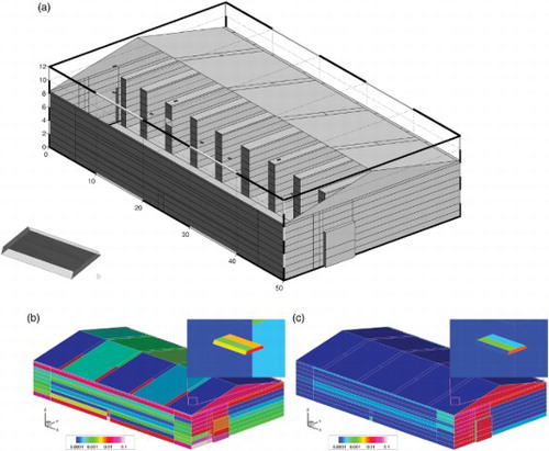
The second scene is a warehouse equipped with ceramic infrared heaters (Figure 7(a)). The warehouse itself has dimensions $50\mathrm{m}\times 30\mathrm{m}\times 12\mathrm{m}$ and contains 9 storage racks. Its surface and the one of the racks is discretized into 700 elements as shown in Figure 7(a). The heaters contribute 100 surface elements. The heaters in the warehouse have a base plate of $0.5\mathrm{m}\times 0.25$ m, i.e. an area of 0.125 m², fitted with reflection shields of a height of 0.05 m (cf. inset in Figure 7(a)). The size of the heaters is determined by the manufacturer's specifications and by a heat load calculation according to DIN EN 12831 (DIN EN 12831 2003).

Figure 7. (a) Surface mesh of the warehouse. Some of the elements have been removed for view of the inside. The details of the geometry of the ceramic infrared heaters are shown on the lower left. For further details see text. (b), (c) Distribution of errors in weighted column sums. On most of the surface elements the error is in the range from 1e−5 to 1e−3. The outliers are located on only a few elements which all feature singularities of the view factor kernel at some of their boundaries. Note the logarithmic scale bars. Surprisingly, the weighted column sums on the infrared heaters converge well, (b) Gauss3, N_tx=1024, n_s=3 and (c) Gauss3, N_tx=1024, n_s=7.

4.2. Error measures

For the A2A view factors of the unit cube and the concentric cubes (for the latter cf. the table in Figure 5(b)), we compute the relative error in per cent

$\delta F_{i\to j}=\frac{|F_{i\to j}-F_{i\to j}^h|}{F_{i\to j}}\cdot 100.$

The results are shown in Figures 8 and 9.

Figure 8. Relative errors of the A2A view factors for the unit cube. The view factor between opposing faces is F_ops and F_adj is the one for surface elements sharing an edge. For reasons of symmetry there are only two mutually different view factors. In all cases the best absolute errors were of the order of 10⁻⁶. The legend of sub-figure (b) applies to all. (a) F_adj, exact value: 0.200044 and (b) F_ops, exact value: 0.199825.

Figure 9. Relative errors of the A2A view factors for the concentric cubes as used in Francisco et al. (2013) (cf. Figure 5(a)). Our results are several orders of magnitude more accurate than those given in Francisco et al. (2013, Table 5 and Figure 13). In all cases the best absolute errors were of the order of 10⁻⁶. The legend of sub-figure (a) applies to all. (a) F_1→I, exact value: 0.079704; (b) F_1→II, exact value: 0.007852; (c) F_I→1, exact value: 0.717336; and (d) F_II→1, exact value: 0.070666.

The HC method computes one row of the view factor matrix at a time and tightly couples the computation of the individual view factors. Thus, instead of merely looking at the errors of individual view factors, we additionally consider a more global error quantity, the deviation from unity of the area-weighted column sums (AWCS),

$\sum _i\frac{A_i}{A_j}{F}_{A_i\to A_j}\stackrel{!}{=}1\mathrm{\forall }j.$

In contrast to Equation (12), this equation can also be used for scenes for which no exact view factors are available. It essentially states that no energy is lost in the transfer from the distant surfaces ${\mathbf{A}}_{\mathbf{i}}$ to an individual surface ${\mathbf{A}}_{\mathbf{j}}$, i.e. there is no unintentional loss of irradiance. For the realistic scenes we have mapped the AWCS to the corresponding ${\mathbf{A}}_{\mathbf{j}}$ which is displayed in Figures 6 and 7 for various values of N_tx and n_s. Equation (13) follows from the reciprocity relation

$A_i{F}_{A_i\to A_j}=A_j{F}_{A_j\to A_i}$

and the fact that the row sums of the exact A2A view factors always fulfil

$\sum _j{F}_{A_i\to A_j}=1\mathrm{\forall }i.$

By construction, the row sums of the P2A view factors obtained from the HC method by means of Equation (8) fulfil Equation (15). This carries over to the A2A view factors in Equation (11). Hence, the row sums are conserved even for the numerically obtained A2A view factors. The factors A_i and A_j are a result of the integration over the surface element from which the other surfaces are viewed. Thus, the constraints on the AWCS apply to the obstructed case as well.

Additionally, we compute the error in the radiant flux balance after solving the corresponding RHT problem. Both errors are measured as function of the HC dimension N_tx and the number of quadrature subdivisions n_s. The radiant flux balance is computed from the electrical network analogy as described in Modest (2003, Sec. 5.4) or Elsner, Fischer, and Huhn (1993).

4.3. Quality of A2A view factors

The computation of the P2A view factors by means of the HC method corresponds to an approximation of the integral in Equation (3) by the box rule. Hence, the error in the integration must be proportional to the texel diameter H.

4.3.1. Error estimate for the HC

Doubling the HC resolution should reduce the error by a factor of two on average. This can be observed in Figure 8(a) and 8(b) for the empty unit cube and 9(a)–9(d) for the concentric cubes, respectively. The influence of the HC resolution is mainly an aliasing error arising from approximating element boundaries which are oblique with respect to the regular grid on the HC surface or which are offset by a fraction of a texel from the grid lines as sketched in Figure 10. The latter is the situation which is solved by refining the HC most easily. In the worst case, a row or column of texels, i.e. N_tx texels, is assigned to the wrong surface element. As Figure 10 indicates this is most severe if the edge of the projection of a surface element is exactly half way in between (dashed line) the grid lines (solid lines) of the HC. To estimate the resulting worst-case error assume that only the lid of the HC is concerned. Then an upper bound for the aliasing error is $0.5\cdot N_{\mathrm{tx}}\cdot 2/N_{\mathrm{tx}}^2$. The factor 0.5 is due to the worst-case positioning of the edge of the surface element half-way in between the grid lines. The area of one texel is $4/N_{\mathrm{tx}}^2$. Hence an upper bound for the P2Tx view factors is $4/\pi /N_{\mathrm{tx}}^2<2/N_{\mathrm{tx}}^2$ which is obtained by approximating the integral in Equation (3) by the box rule. Since we neglected the angular dependence of the P2Tx view factors on the lid, we have grossly overestimated the upper bound. Therefore, we can safely assume that this upper bound in practice also covers the error contributions from the walls of the HC. In case of oblique edges, the aliasing errors due to the individual texels intersecting the edge should roughly cancel each other. Hence, the error should be close to 1/N_tx. Since it is no problem to choose $N_{\mathrm{tx}}=4096$ or 8192 on modern GPUs, this is simply not an issue and for practical purposes the P2A view factors computed by Equation (8) can be considered as exact.

Figure 10. Effect of a mismatch between the HC grid and the edge of the projection of a surface element onto the HC. Details see text.

4.3.2. Influence of numerical integration

The calculation of A2A view factors by numerical quadrature according to Equation (9) requires the assessment of a second source of error: the approximation properties of the quadrature rule used for the integration over the surface element ${\mathbf{A}}_{\mathbf{i}}$. Basically, we have two choices. Either we use a quadrature rule which is able to integrate polynomials of high order exactly or we use a low-order quadrature rule and subdivide the surface element ${\mathbf{A}}_{\mathbf{i}}$ into subsurfaces so that the final A2A view factor is the sum of the A2A view factors of the subsurfaces (cf. Equation (11) and Figure 3). This corresponds to the h-refinement strategy in finite elements which is especially useful for integrands with singularities. In the case of view factor computations, singularities arise from surface elements which have a common edge (e.g. faces 1 and 2 in Figure 5(a)) or corner. The contribution of the quadrature rule is revealed by the saturation of the relative view factor error for high HC resolutions (meaning large N_tx) for a given quadrature subdivision n_s (cf. Figure 9(a)–9(d)). This effect becomes particularly apparent in the case of small elements viewed from large elements (Figure 9(a) and 9(b)). This is also reflected in the deviations from unity of the extremal AWCS in the bottom part of Figure 11. There we plot

$\underset{j}{max}\sum _i\frac{A_i}{A_j}{F}_{A_i\to A_j}-1,1-\underset{j}{min}\sum _i\frac{A_i}{A_j}{F}_{A_i\to A_j}$

Figure 11. Top: Total CPU times vs. HC dimension for computing the A2A view factor matrix of the concentric cubes (cf. Figure 5(a)). Bottom: Deviation from unity of the largest and the smallest column sum of the A2A view factor matrix. The column sums are computed from Equation (13). The legend in the top figure applies to all sub-figures.

as function of the HC dimension N_tx and the number of steps of quadrature subdivision n_s=0, 1, 2, 3. The closer to zero the better the values are. The same is done for the warehouse in Figure 12.

Figure 12. Deviation from unity of the weighted column sums in case of the warehouse computed on c3, cf. Figure 7(a) and Table 2. We plot the extrema as function of the HC dimension N_tx and the level of quadrature subdivision n_s.

Figure 13. Achieved PCIe transfer rates for the warehouse (cf. Figure 7(a)).

The other case of large solid angles subtended by the distant surface element shows that the aliasing error due to the HC method dominates and increasing n_s has less impact (Figure 9(c) and 9(d)).

Figure 12 clearly shows that in order to minimize the error in the AWCS of the view factor matrix one rather needs a high subdivision n_s of the quadrature rule than a very large HC dimension N_tx. This can be understood by the same argument brought forward to explain the convergence behaviour for the view factors F_1→I and F_1→II of the concentric cubes. However, if the HC is too coarse, high values for n_s are futile as well.

In our tests, we used 1-, 3-, 4- and 7-point Gauss–Legendre quadrature rules on triangles. Of those the 3-point rule has proven to be the most economic in terms of speed and accuracy. Hence, we mostly show the results for the 3-point rule, except for the test cabin for which we use the 7-point Gauß rule (cf. Table 3). Details on the performance of different quadrature rules will be presented elsewhere.

Table 3.  Barycentric coordinates (p_x, p_y, p_z) and weights w_α of the 7-point Gauss–Legendre quadrature on a triangle.

px	py	pz	w
1/3	1/3	1/3	0.22500000
0.05961587	0.47014206	0.47014206	0.13239415
0.47014206	0.05961587	0.47014206	0.13239415
0.47014206	0.47014206	0.05961587	0.13239415
0.79742699	0.10128651	0.10128651	0.12593918
0.10128651	0.79742699	0.10128651	0.12593918
0.10128651	0.10128651	0.79742699	0.12593918

Note: Weights are normalized such that their sum equals one.

4.4. Efficiency of the implementation

We measure the efficiency of the implementation by comparing the achieved data transfer rates with their theoretical maximums. We have to consider two different data transfers: from the framebuffer into the pixel buffer (step 1 in Figure 4), an intra-GPU operation, and from the pixel buffer to its mirror in the main memory on the CPU side which is realized as DMA transfer across the PCIe bus (step 2 in Figure 4). The latter is the performance limiting step. This can already be inferred from the theoretical values. Intra-GPU memory transfers take place at a rate of 50–250 GB/s, whereas depending on the number of PCIe lanes with which the GPU is connected to the PCIe bus, the maximum PCIe transfer rate is 4–5 GB/s. Hence, we only consider the PCIe transfer rate achieved in practice:

$\begin{array}{rl}{k}_{\mathrm{PCIe}}& :=\frac{n_{\mathrm{HC}}\cdot 3\cdot N_{\mathrm{tx}}^2\cdot 3\mathrm{bytes}}{\mathrm{total}\mathrm{CPU}\mathrm{time}}\end{array}$

$\begin{array}{rl}{n}_{\mathrm{HC}}& :=n_p\cdot n_q\cdot 4^{n_s},\end{array}$

where n_HC is the total number of HC to render, n_p is the number of elements in the surface mesh, $3N_{\mathrm{tx}}^2$ is the total number of texels on the HC and n_q is the number of quadrature points on the reference triangle. Because of the small number of surface elements in our scenes we omitted the α channel in the colour coding of the element index which reduces the amount of data per texel to 3 bytes. On all machines used in our tests the maximum achieved PCIe transfer rate k_PCIe reached 1–1.7 GB/s. As a typical example we show the dependence of k_PCIe on the HC dimension N_tx for the warehouse on the machine c3 in Figure 13. The exact value of k_PCIe depends on the speed and bus width of the GPU memory and whether the CPU is able to finish the summation of the P2Tx view factors according to Equation (8) within the time needed for the DMA transfer from the GPU to the main memory.

The total CPU times for the unit cube and concentric cubes on retina are shown in the top part of Figures 14 and 11, respectively, and the CPU times for the warehouse on c3 in Figure 15. All show that for fine-grained HCs the run times approach the asymptotic behaviour of being proportional to the number of texels on the top of the HC, $N_{\mathrm{tx}}^2$. For coarse-grained HCs the run times are roughly constant since the overhead in the PCIe transfer dominates. PCIe transfer rates start to saturate for HC dimensions, N_tx>256. The onset of this saturation depends on the number of surface elements. If the computation is distributed over several machines, the total runtime is the corresponding fraction of the single-machine runtime.

Figure 14. Top: Total CPU times vs. HC dimension for the computation of the A2A view factor matrix of the unit cube. Bottom: Deviation from unity of the largest and the smallest column sum of the A2A view factor matrix. The column sums are computed from Equation (13). The legend in the top figure applies to all sub-figures.

Figure 15. Dependence of the total run time on the HC dimension and quadrature subdivision for the warehouse on c3 (cf. Figure 7(a) and Table 2). For coarse-grained HCs the run time is roughly constant since the overhead in the PCIe transfer dominates. PCIe transfer rates start to saturate for HC dimensions larger than 256.

Figure 16. Relative error of the radiant flux balance for the warehouse (cf. Figure 7(a)).

Hardware-accelerated rendering, the parallelization of data transfers and summation of P2Tx view factors enable us to compute the view factor matrix for the cube scenes in a fraction of a second up to roughly a minute, depending on the level of the quadrature subdivision, n_s. This is approximately a thousand times faster than in a previous, independent study (Francisco et al. 2013). This speedup cannot be attributed to possible differences in the CPUs used, but rather has to be explained by the hardware-accelerated visibility testing. Our runtime plots also show that the total CPU times quadruple with each quadrature subdivision, reflecting the four-fold increase of the number of quadrature points, i.e. the natural complexity of the algorithm. Although not explicitly shown here, the complexity w.r.t. to n_p is linear and to some extent comparable to HR (Hanrahan, Salzman, and Aupperle 1991).

4.5. Error of radiant flux balance

The radiant flux balances are computed with TRNSYS-TUD (Perschk 2000), a modification and extension of TRNSYS, version 14.2 (University of Wisconsin-Madison, Solar Energy Laboratory and Klein 1979). In both test cases, warehouse and test cabin, the error seems to converge to a finite value (cf. Figures 16 and 17). Because of the exponential growth of the runtime with the number of quadrature subdivisions n_s (cf. Equation (18)), we are limited to n_s≤7. For instance, on c4 a computation for the warehouse with the 3-point quadrature rule, an HC dimension $N_{\mathrm{tx}}=1024$ and n_s=5, we need a total runtime of 15 hours (cf. Figure 15) to achieve an error of 0.56 kW in the radiant flux balance. This corresponds to a relative error of 0.5% of the total power of 120.8 kW of the heating system. Increasing the subdivision to n_s=6 quadruples the runtime, yet the error is reduced only by 0.02 kW. Thus, there is only a little effect on the relative error. This is a drastic improvement both in speed and accuracy. With a former non-GPU implementation in TRNSYS-TUD a comparable computation takes 700 hours and the error in the radiant flux balance is roughly an order of magnitude larger. The distribution of the AWCS for the warehouse for two different refinement levels n_s of the 3-point Gauß rule is shown in Figure 7(b) (n_s=3) and 7(c) (n_s=7). In both cases the HC dimension is set to $N_{\mathrm{tx}}=1024$.

Figure 17. Relative error of the radiant flux balance for the test cabin with radiator section (cf. Figure 6(a)). Despite an error of at least 30% in the weighted column sums (cf. Equation (13)), the radiant flux balance is violated only by about 4%.

Another conclusion to be drawn from Figure 16 is that one can obtain good results even for coarser HCs provided n_s is sufficiently large. Taking into account that for small HC dimensions the PCIe transfer rates do not saturate, there is still room for further speedups by merging the DMA transfers of many small HCs into one by copying several framebuffers into corresponding tiles of only one pixel buffer.

For the test cabin the extremal errors of the AWCS of the view factor matrix converge towards 0.63 and 1.01, respectively, yet the error in the radiant flux balance is only 5%. This shows that although the column sum errors are a reasonable criterion for the error they are not able to completely track the propagation of errors. One way to assess the importance of a particular surface for the error in the radiant flux balance is to use Equation (9) in Section 5.1 of Lischinski, Smits, and Greenberg (1994). The distribution of the AWCS errors for the test cabin is shown in Figure 6(b)–6(d). Figure 6(b) shows the distribution of the AWCS on the walls of the cabin itself. Even at the wall close to the radiator most AWCS are of the order of 10⁻⁵ to 10⁻³. The most notable deviations occur in the corners where the view factor kernel has its singularities. In Figure 6(c), the walls of the cabin are semi-transparent in order to allow a simultaneous assessment of the AWCS on the surface of the radiator segment and the walls of the cabin. Figure 6(d) shows the radiator in detail and highlights that even for the thin convection fin the AWCS are still of a reasonable accuracy except for two pathological surface elements of the upper edge where the convection fin is attached to the body of the radiator. Given the complexity of the geometry and the large range of aspect ratios and the size distribution of the surface elements we consider this as a remarkable result. Especially in the light of the fact that except for the two pathological surface elements on the upper edge, the total error in the AWCS for this complex scene is as large as the error in the view factor of an individual pair of surface elements as, e.g. in Walton (2002).

5. Conclusion

The combination of an OpenGL-based implementation of the HC algorithm and current parallel programming techniques enables us to fully exploit the enormous compute power of modern graphics cards and multi-core CPUs. Especially the visibility testing profits from this approach as it is done in hardware and can be implemented by a few lines of OpenGL.

The parallel pipelining of rendering the HC, data transfers between graphics card and CPU, and the summation of P2Tx to eventually A2A view factors allow us to utilize most of the theoretically possible performance of current hardware. Furthermore, the computational time of our approach scales well when the computation is distributed over several machines. From our numerical experiments, we infer that an HC resolution of $1024\times 1024$ texels is sufficient for practical purposes and that beyond that the P2A view factors can be considered as exact.

On hardware platforms where CPU and GPU address the same physical memory, our algorithm could be further simplified as then there would be no need to actually copy the HC data. Rather, the different parts of the program would just have to exchange pointers which eliminates the bottleneck imposed by the PCIe bus. Currently, such architectures exist only for the low-cost market, e.g. AMD's Fusion architecture and its descendants, so that even with proper modifications our program would most likely be slower because of the low-performance CPU and GPU packed into these hybrid architectures.

We have shown that the benefit of a careful parallelization and exploitation of hardware acceleration is an increased accuracy of the view factors and an improvement of the radiant flux balance compared to previous implementations.

Our high-performance implementation is optimal in the sense of exhausting hardware capabilities, especially memory transfer rates over the PCIe bus. As a by-product our work yields an accurate and fast method to compute the numerous P2A view factors needed for the coupling of building performance simulations and CFD simulations of indoor air flow. An interesting extension of our work would be to combine the contour integral approach with hardware-accelerated visibility testing, especially for surface elements with large aspect ratios.

Having accurate view factors for individual pairs of surface elements is elemental, but for practical purposes like thermal comfort predictions this is not enough. We have shown that the error in the radiant flux balance for realistic use cases can be improved by an order of magnitude while the needed computational time is reduced by up to three orders of magnitude. The savings in run time are also observed when comparing our results with an entirely independent implementation (Francisco et al. 2013). The analysis of the AWCS of the view factor matrix shows that even in complex geometries with a broad range of aspect ratios and sizes of surface elements it is possible to obtain accurate A2A view factors within a reasonable amount of time. Yet, our requirements on the computational resources are only moderate.

Acknowledgement

We thank Gert Lube for many fruitful discussions and for his continuous and long-standing, encouraging support.

References

- Bangerth, Wolfgang, Ralf Hartmann, and Guido Kanschat. 2007. “Deal.II – A General Purpose Object Oriented Finite Element Library.” ACM Transactions on Mathematical Software 33 (4): 24/1–24/27. doi: 10.1145/1268776.1268779
- Bao, H., and Q. Peng. 1994. “An Efficient Form-Factor Evaluation Algorithm for Environments with Curved Surfaces.” Computers & Graphics 18 (4): 481–486. doi: 10.1016/0097-8493(94)90060-4
- Blanchette, J., and M. Summerfield. 2008. C++ GUI Programming with Qt 4. Upper Saddle River, NJ: Prentice Hall PTR.
- Bopche, S. B., and A. Sridharan. 2009. “Determination of View Factors by Contour Integral Technique.” Annals of Nuclear Energy 36 (11–12): 1681–1688. doi: 10.1016/j.anucene.2009.09.007
- Cohen, M. F., and D. P. Greenberg. 1985. “The Hemi-Cube: A Radiosity Approach for Complex Environments.” Computer Graphics 19 (3): 3–40. doi: 10.1145/325165.325171
- Cohen, M., J. Wallace, and P. Hanrahan. 1993. Radiosity and Realistic Image Synthesis. San Diego, CA: Academic Press Professional, Inc.
- Coombe, G., M. J. Harris, and A. Lastra. 2004. “Radiosity on Graphics Hardware.” Proceedings of graphics interface 2004, GI ’04, London, Ontario, Canada School of Computer Science, University of Waterloo, 161–168. Waterloo, Ontario: Canadian Human-Computer Communications Society.
- DIN EN 12831. 2003. Heating Systems in Buildings – Method for Calculation of the Design Heat Loads. Berlin: Beuth Verlag. [German version].
- DIN EN 442-2. 2003. Radiators and Convectors – Part 2: Test Methods and Rating. Berlin: Beuth Verlag. [German version].
- Dobrowolski de Carvalho Augusto, L., B. Giacomet, and N. Mendes. 2007. “Numerical Method for Calculating View Factor Between Two Surfaces.” Proceedings: Building Simulation 2007. Accessed 2007. http://www.ibpsa.org/proceedings/BS2007/p757_final.pdf.
- Dudka, K. 2007. “RRV: Radiosity Renderer and Visualizer.” Accessed June 6, 2009. http://dudka.cz/rrv.
- Elsner, N., S. Fischer, and J. Huhn. 1993. Grundlagen der Technischen Thermodynamik, Band 2 Wärmeübertragung. 8th ed. Berlin: Akademie Verlag.
- Faghri, A., Y. Zhang, and J. Howell. 2010. Advanced Heat and Mass Transfer. Columbia, MO: Global Digital Press.
- Feng, Y., and K. Han. 2012. “An Accurate Evaluation of Geometric View Factors for Modelling Radiative Heat Transfer in Randomly Packed Beds of Equally Sized Spheres.” International Journal of Heat and Mass Transfer 55 (23–24): 6374–6383. doi: 10.1016/j.ijheatmasstransfer.2012.06.025
- Francisco, S. C., A. M. Raimundo, A. R. Gaspar, A. V. M. Oliveira, and D. A. Quintela. 2013. “Calculation of View Factors for Complex Geometries Using Stokes’ Theorem.” Journal of Building Performance Simulation 7 (3): 1–14. 10.1080/19401493.2013.808266.
- Goral, C. M., K. E. Torrance, D. P. Greenberg, and B. Battaile. 1984. “Modeling the Interaction of Light Between Diffuse Surfaces.” Proceedings of the 11th annual conference on computer graphics and interactive techniques, SIGGRAPH ’84, 213–222. New York: ACM.
- Hammer, P. C., O. J. Marlowe, and A. H. Stroud. 1956. “Numerical Integration Over Simplexes and Cones.” Mathematical Tables and Other Aids to Computation 10 (55): 130–137. doi: 10.2307/2002483
- Hanke, M. 2009. “Multithreaded-OpenGL Rendering with Picking in Qt.” Accessed September 13, 2009. http://mih.voxindeserto.de/threadedcube.html
- Hanrahan, P., D. Salzman, and L. Aupperle. 1991. “A Rapid Hierarchical Radiosity Algorithm.” SIGGRAPH Computer Graphics 25 (4): 197–206. doi: 10.1145/127719.122740
- Howell, J. 1982. A Catalog of Radiation Configuration Factors. New York, NY: McGraw-Hill Ryerson.
- Jones, N. L., D. P. Greenberg, and K. B. Pratt. 2012. “Fast Computer Graphics Techniques for Calculating Direct Solar Radiation on Complex Building Surfaces.” Journal of Building Performance Simulation 5 (5): 300–312. doi: 10.1080/19401493.2011.582154
- Kim, T., S. Kato, and S. Murakami. 2001. “Indoor Cooling/Heating Load Analysis Based on Coupled Simulation of Convection, Radiation and HVAC Control.” Building and Environment 36 (7): 901–908. doi: 10.1016/S0360-1323(01)00016-6
- Kobayashi, K., J. Nakano, Y. Ozeki, and M. Konishi. 2002. “Evaluation of Thermal Comfort Using Combined Multi-node Thermoregulation (65MN) and Radiation Models and Computational Fluid Dynamics (CFD).” Energy and Buildings 34 (6): 637–646. doi: 10.1016/S0378-7788(02)00014-2
- Koch, R., and R. Becker. 2004. “Evaluation of Quadrature Schemes for the Discrete Ordinates Method.” Journal of Quantitative Spectroscopy & Radiative Transfer 84 (4): 423–435. doi: 10.1016/S0022-4073(03)00260-7
- Lischinski, D., B. Smits, and D. P. Greenberg. 1994. “Bounds and Error Estimates for Radiosity.” Proceedings of the 21st annual conference on computer graphics and interactive techniques, SIGGRAPH ’94, 67–74. New York: ACM.
- Lube, G., T. Knopp, G. Rapin, R. Gritzki, and M. Rösler. 2008. “Stabilized Finite Element Methods to Predict Ventilation Efficiency and Thermal Comfort in Buildings.” International Journal for Numerical Methods in Fluids 57 (9): 1269–1290. doi: 10.1002/fld.1790
- Lum, E., K. L. Ma, and N. Max. 2002. “Interactive Radiosity Using Mipmapped Texture Hardware.” In 13th Eurographics Workshop on Rendering: Pisa, edited by S. Gibson and P. Debevec, Italy, June 26–28, Vol. 28 of ACM International Conference Proceeding Series. Aire-la-Ville, Switzerland: Eurographics Association.
- Lum, E. B., K. L. Ma, and N. Max. 2005. “Calculating Hierarchical Radiosity form Factors Using Programmable Graphics Hardware.” Journal of Graphics, GPU, and Game Tools 10 (4): 61–71. doi: 10.1080/2151237X.2005.10129210
- MacFarlane, J. J. 2003. “VISRAD – A 3-D View Factor Code and Design Tool for High-Energy Density Physics Experiments.” Journal of Quantitative Spectroscopy and Radiative Transfer 81 (1–4): 287–300. doi: 10.1016/S0022-4073(03)00081-5
- Max, N. 1995. “Optimal Sampling for Hemicubes.” IEEE Transactions on Visualization and Computer Graphics 1 (1): 60–76. doi: 10.1109/2945.468388
- Mishra, S. C., H. K. Roy, and N. Misra. 2006. “Discrete Ordinate Method with a New and a Simple Quadrature Scheme.” Journal of Quantitative Spectroscopy & Radiative Transfer 101 (2): 249–262. doi: 10.1016/j.jqsrt.2005.11.018
- Modest, M. F. 2003. Radiative Heat Transfer. 2nd ed. San Diego, CA: Academic Press.
- Perschk, A. 2000. “Gebäude-Anlagen-Simulation unter Berücksichtigung der hygrischen Prozesse in den Gebäudewänden.” PhD diss., Technische Universität Dresden.
- Schröder, P., and P. Hanrahan. 1993. “On the Form Factor Between Two Polygons.” Proceedings of the 20th annual conference on computer graphics and interactive techniques, SIGGRAPH ’93, 163–164. Anaheim, CA: ACM.
- Smits, B. E., J. R. Arvo, and D. H. Salesin. 1992. “An Importance-Driven Radiosity Algorithm.” Proceedings of the 19th annual conference on computer graphics and interactive techniques, SIGGRAPH ’92, 273–282. New York: ACM.
- Stroud, A. H. 1971. Approximate Calculation of Multiple Integrals. Prentice-Hall Series in Automatic Computation. Englewood Cliffs, NJ: Prentice-Hall.
- Swaminarayan, S., and J. Turner. 2007. A Novel Single Projection Method to Calculate View Factors for Radiosity, and a GPU-Based Implementation in a Large Multiphysics Code. Technical Report LALP-07-041. Los Alamos, NM: Los Alamos National Laboratory.
- University of Wisconsin-Madison, Solar Energy Laboratory, and S. A. Klein. 1979. TRNSYS, a Transient System Simulation Program. Madison, WI: Solar Energy Laboratory, University of Wisconsin-Madison.
- Walton, G. N. 2002. Calculation of Obstructed View Factors by Adaptive Integration. Technical Report NISTIR-6925. Gaithersburg, MD: National Institute of Standards and Technology.
- Walton, G. N., and J. Pye. 2011. “View3D.” Accessed July 26, 2013. http://view3d.sourceforge.net/
- Wilson, G., and P. Lu. 1996. Parallel Programming Using C++. Scientific and Engineering Computation. Cambridge, MA: MIT Press.