Spawn: coupling Modelica Buildings Library and EnergyPlus to enable new energy system and control applications

Abstract

Spawn is DOE's next-generation tool chain for whole building energy control simulation. Spawn couples traditional imperative load-based envelope modelling with new equation-based modelling of HVAC and controls. Spawn uses EnergyPlus for the former and the Modelica Buildings Library for the latter. Because it leverages the Modelica Buildings Library, Spawn can evaluate advanced energy systems at the building and district scale, including new architectures and controls for heat pump systems with storage, and the coupling of such systems to electrical distribution networks. Spawn's Modelica integration likewise enables it to simulate realistic control sequences and therefore to bridge energy simulation and control implementation workflows. From EnergyPlus, Spawn inherits efficient envelope simulation and the ability to use existing envelope model authoring tools. This paper describes the architecture and implementation of Spawn, which automatically couples Modelica and EnergyPlus for run-time data exchange. This paper closes with examples that illustrate Spawn's modelling and simulation processes.

Keywords:

• Modelica
• EnergyPlus
• building energy simulation
• controls
• co-simulation
• modular modelling

1. Introduction

Spawn is DOE's next-generation whole building energy-control simulation tool chain. Spawn's overarching purpose is to bridge the currently separate domains of whole-building energy simulation and building control implementation. From Modelica, Spawn draws the ability to simulate realistic controls (i.e. as they are written in the real world), allowing real-world control sequences to be tested, evaluated and optimized for energy performance in simulation before being installed in the target building. Unlike previous Modelica-only implementations (Wetter et al. 2022; Zhang et al. 2020), Spawn integrates the EnergyPlus envelope model to leverage both efficient envelope simulation and mature envelope model authoring tools. Put simply, EnergyPlus (Crawley et al. 2001) is used by Spawn to model and simulate building envelopes, while the Modelica Buildings Library (Wetter et al. 2014) is used to model HVAC systems and their controls. This paper introduces Spawn, describes its architecture, explains the motivation for major decisions underlying its design and illustrates its function and applications using simple examples.

EnergyPlus and Modelica use fundamentally different modelling approaches and simulation technologies that are tailored to different applications and have complementary strengths and limitations. Spawn combines these approaches in a way that applies each approach to the simulation sub-domain in which it is strong.

EnergyPlus has well-established envelope, daylighting and load simulation models, as well as a robust ecosystem of associated authoring tools. Modelica's envelope model authoring tools are lagging. Moreover, while native building envelope models exist in various Modelica libraries, they increase translation times, and simulation times are also higher compared to using EnergyPlus envelope simulation coupled to Modelica (Wetter, Benne, and Ravache 2021). Efforts to reduce translation times and to address simulation time scaling using multi-rate solvers are ongoing, but for now, these drawbacks persist.

The situation is reversed in the HVAC sub-domain. EnergyPlus has a comprehensive set of HVAC component models but also some fundamental restrictions – derived from sequential load-based simulation of primary and secondary loops – on the topologies in which these components can be assembled into systems. These restrictions prevent it from modelling certain novel energy systems including two-pipe systems for simultaneous heating and cooling (Maccarini et al. 2017) and reservoir district energy networks (Sommer et al. 2020). Modelica is an open standard for modelling of engineered systems (Mattsson, Otter, and Elmqvist 1999); in the buildings domain, its strength is in modelling thermal and electrical energy systems for both single buildings and multi-building districts. In Modelica, there are no topological restrictions, so any energy system configuration can be modelled. Modelica models exist for the systems mentioned above as well as for geothermal district systems (Gautier, Wetter, and Sulzer 2022; Laferrière et al. 2020).

Modelica has an even more significant and fundamental advantage when it comes to modelling HVAC controls. EnergyPlus performs traditional, quasi-static, load-based simulation. This approach requires HVAC operation and the control decisions that drive it to essentially be applied ‘retroactively’ within each time step. Consider the steps EnergyPlus follows to control a cooling coil: (i) it tabulates the heat that will be added to a zone during the time step, (ii) it uses this heat to calculate the value that the zone temperature will have at the end of the time step, (iii) if the zone temperature exceeds the cooling set point, it reasons that the cooling system must have activated during the time step to remove the excess heat, (iv) it calculates the cooling system's required average (part load) operation over the time step to remove the heat and (v) it recalculates the zone's new state using the combined effects of the externally added heat and the heat removed by the cooling system. In contrast, real-world control is expressed to reduce control errors, i.e. the difference between a set point and a measurable quantity, in real time. The fact that control sequences in EnergyPlus are different than their real-world counterparts introduces significant friction in terms of time, effort, human error and ultimately cost, into the control delivery and implementation process. Control sequences selected during project design using EnergyPlus cannot be handed off to a control implementation engineer in a portable digital form. Instead, they are described using text and diagrams which the engineer must then interpret and re-implement.

Modelica supports dynamic simulation of HVAC operation and control models that are formulated using differential equations describing the rates of change of state variables, such as zone air temperature or the integral term of a PI controller, along with discrete equations that describe when equipment switches the mode of operation and algebraic equations that are used to calculate, for example, the air- or water-flow distribution in duct and pipe networks based on flow friction. To simulate such systems, in Modelica tools, one typically uses solvers that adapt the time step length to meet an error tolerance. Long time steps are used when dynamics are slow, and shorter time steps are used when dynamics are fast and when needed to properly find the time instant at which control switches the operation modes of equipment. The trajectories of quantities such as temperature and flow rate evolve based on the feedback response of control logic that may determine positions of actuators and speeds of fans and pumps. An important consequence of this approach is that Modelica can correctly simulate physically-realistic feedback control sequences of the kind used in real buildings. This enables the development of digitized control delivery processes that leverage the same control sequence representations for both simulation-based correctness testing, performance evaluation and optimization on one end, and bidding, translation to commercial control product lines, formal verification and commissioning on the other. A Modelica subset called Control Description Language (Wetter, Grahovac, and Hu 2018), which is being standardized in ASHRAE Standard 231P, is the control representation that enables this automation (Wetter et al. 2022). See Roth et al. (2022) for an extension of this work that further automates the workflow based on semantic models.

Also, various Modelica libraries that allow modelling the design and operation of integrated energy systems in which electrical systems, power generation, and energy conversion and storage across energy carriers are tightly integrated (Baetens et al. 2012; Baudette et al. 2018; Bonvini, Wetter, and Nouidui 2014; Casella and Leva 2003; MacRae et al. 2020; Senkel et al. 2021) to improve performance. The Modelica Buildings Library also contains models for geothermal heat exchangers and borefields, and an interface to the subsurface simulator TOUGH (Doughty et al. 2021; Hu et al. 2020).

As Modelica is an open standard, users can benefit from a large ecosystem of modelling tools and simulation backends, domain-specific libraries, related open standards such as the Functional Mockup Interface Standard (FMI) (Blochwitz et al. 2012), System Structure and Parameterization (SSP) (Modelica Association 2019), Distributed Co-Simulation Protocol (DCP) (Krammer et al. 2019) or the eFMI Standard for physical models in embedded software (Lenord et al. 2021). End users can benefit from the ecosystem's open standards because they can avoid being locked in into using a particular proprietary software provider.

Using Modelica also allows open collaboration on model development, as has been done through the IEA EBC Annex 60 project (Wetter and van Treeck 2017), through the IBPSA Project 1 (Wetter, van Treeck et al. 2019) and now through the IBPSA Modelica Working Group (Wetter 2022). These collaborative projects have led, for example, to the Modelica IBPSA Library (Wetter et al. 2015), which is now the basis of four Modelica libraries for building and district energy systems, namely AixLib (Müller et al. 2016), Buildings (Wetter et al. 2014), BuildingSystems (Nytsch-Geusen et al. 2013) and IDEAS (Jorissen et al. 2018).

2. Scope of Spawn

Spawn simulates the fundamental physical phenomena needed to accurately evaluate building energy use, including heat and moisture transfer through the building fabric, daylighting, natural ventilation, pressure-driven flow distribution in ducts and pipe networks. Spawn can be used to model HVAC systems, district heating and cooling systems, electrical systems and occupant behaviour. It can model idealized and actual control sequences. These capabilities support the following use cases:

1. Annual simulation of energy demand by buildings and district energy systems such as in Gautier, Wetter, and Sulzer (2022).

2. Equipment sizing using parameter sweeps or optimization. Modelica development environments generally have built-in support for optimization (Åkesson et al. 2010; Dietl et al. 2014; Fritzson et al. 2020; Pfeiffer 2012), which can be used to optimally size HVAC equipment and storage, or, alternatively, an external optimizer can be wrapped around a Modelica model. Moreover, the Modelica language allows sizing calculations to be embedded in parameter assignments that set equipment, pipe, valve and duct sizes.

3. Controls design, including comparing the performance of different realistic building control sequences such as shown in Zhang et al. (2020) and Zhang et al. (2022), or optimization-based control tuning using the optimization features listed in the above item.

4. Export of control sequence for implementation in building automation systems and for verification of as-installed sequences relative to the design specification (Wetter et al. 2022; Wetter, Gautier et al. 2019; Wetter, Grahovac, and Hu 2018). Also, in Spawn, controls and the mechanical system is implemented using the Modelica language. This enables the use of the FMI Standard that has been developed for tool interoperability (Blochwitz et al. 2012), or the eFMI Standard (Lenord et al. 2021) that has been developed for model-driven development of complex, safety-critical, physics-based embedded control.

5. Extraction of component and subsystem models to execute them in isolation for given input and initial states. This allows, for example, subsystem models to be used (i) as part of a building controller, such as for running a model for model-based design in the Niagara framework of Tridium (Nouidui and Wetter 2014), (ii) for commissioning of as-installed control logic (Wetter et al. 2022; Wetter, Gautier et al. 2019) or (iii) to compute input–output transfer functions, which then can be used to designing a controller in the frequency domain (Bortoff et al. 2022; Wetter 2009).

3. Prior work

The coupling of HVAC system and envelope models from different simulation tools has been demonstrated several times. Chapter 6 of the IEA EBC Annex 60 Final Report (Wetter and van Treeck 2017) gives an overview of various tools that export Modelica HVAC or envelope models and that orchestrate their co-simulation. Other notable couplings include TRNSYS with CONTAM to evaluate building control strategies (Dols, Emmerich, and Polidoro 2016) and TRNSYS with ESP-r (Beausoleil-Morrison et al. 2012).

The Functional Mockup Interface (FMI) Standard is an open standard that can be used to exchange models. FMI defines how to package models in a tool-independent way so that other tools can import the model, can inspect what its parameters, inputs, state variables and outputs are, and can inspect the mathematical properties of the model that are needed to efficiently simulate the model. This is declared in an XML file, which is packaged together with the model in a zip file which is called a Functional Mockup Unit (FMU). FMI is supported by more than 170 tools. The Building Controls Virtual Test Bed (BCVTB) is a co-simulation middleware that can link various building energy and control simulators using the FMI Standard (Wetter 2011). FMI has been used to import Modelica component models into TRNSYS (Elsheikh, Awais et al. 2013; Elsheikh, Widl et al. 2013) and into the WUFI hygrothermal whole building simulation program (Pazold et al. 2012). EnergyPlus itself supports FMI in two ways. First, it has an FMU import interface that allows adding HVAC and control models to the EnergyPlus envelope model, EMS actuators and schedules (Nouidui, Wetter, and Zuo 2014). Second, EnergyPlusToFMU exports EnergyPlus as an FMU for co-simulation (LBNL 2013).

Spawn coupling differs from these earlier systems in two aspects. First, Spawn automatically exports the EnergyPlus envelope model as an FMU, links it to various Modelica models that need to interact with it and sets up the co-simulation synchronization algorithm. This approach requires no FMU export and import tools or co-simulation environment to be set up by the user, reducing complexity.

Second, for computational efficiency, Spawn places the heat and mass balance calculations for room air in the HVAC domain rather than the envelope domain, as earlier work had done. Room air state evolution exhibits fast dynamics at similar time scales to those of the HVAC system. Placing these in different simulation domains from HVAC requires short synchronization time steps that lead to longer simulation times, as we observed in earlier couplings that used the FMU import/export interface of EnergyPlus and the BCVTB. By placing the room air model in the HVAC domain, Spawn allows the dynamics of room air and HVAC to be solved together and minimizes the burden of synchronization with the slower dynamics of the envelope domain.

4. Architecture

This section describes the Spawn architecture, how a model is partitioned into envelope and HVAC domains, how these domains are synchronized, and how the system is packaged for end-users.

4.1. Model domain partitioning

In Spawn, the model domain is partitioned into two subdomains: the envelope model in EnergyPlus and the energy system model, together with the room air heat and mass balance, in Modelica. This partitioning and resulting coupling have the following characteristics:

1. Model authoring: Existing envelope modelling tools can be used to create the EnergyPlus input data file. Modelica model authoring tools can be used to create the HVAC and control models, as well as to specify the coupling between envelope, HVAC and controls.

2. Simulation environment: Any Modelica-compliant simulation environment can be used to simulate Spawn models.

3. Simulation time: The synchronization interval between EnergyPlus and Modelica is maximized by using slowly varying variables, i.e. the room-surface heat transfer. Fast changing variables such as the room air pressure, temperature and mass concentration are modelled in Modelica so that they can be simulated with an adaptive time step solver that can use shorter time steps than used for coupling with the envelope model.

4. Interface specification: The two domains are coupled using the FMI Standard, enabling individual testing of components, reuse of the FMI Library (Modelon 2022) for coupling the software, and reliance on well-tested interface specifications.

The partitioning is shown in Figure 1. Solid lines indicate data that are exchanged at the fixed EnergyPlus zone time step, as specified by the EnergyPlus TimeStep object. Dashed lines indicate that data are sent whenever the Modelica model receives a new value. The individual depicted models that exchange data between Modelica and EnergyPlus are as follows:

Figure 1. Partitioning between the EnergyPlus and Modelica modelling domains.

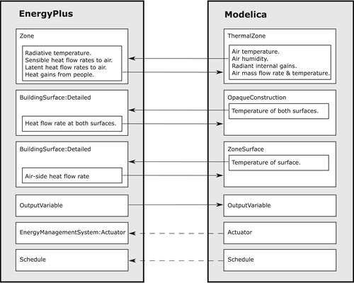
Figure 2. Partitioning of heat and mass balance between Modelica and EnergyPlus.

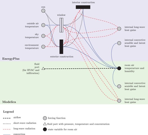
1. Thermal Zone: The Modelica ThermalZone model connects to an EnergyPlus Zone model. Figure 2 shows how the energy balance is split between them. Modelica simulates the air's conservation equations for energy, mass and concentrations of water vapour and trace substances such as CO${}_2$ or VoCs.

   The convective flows are handled as follows: outside air infiltration and interzonal air exchange are modelled in Modelica using the fluidPort connector¹ of the room model, because any infiltration or interzonal air exchange that the EnergyPlus model may specify is ignored. At each coupling time step, EnergyPlus computes the convective sensible and latent heat transfer with the building fabric using the room air temperature and humidity received from Modelica. EnergyPlus then sends the convective heat and mass flow rates to Modelica, which uses them to calculate time rate of change of the room air temperature and humidity concentration. EnergyPlus similarly computes and relays internal heat gains such as from equipment and people, although these can be specified in Modelica as well as the two heat gain specifications are added by Spawn. If people are modelled in EnergyPlus (using the People object) and the Modelica medium model² contains CO2, then the $C{O}_2$ emitted by people is automatically added to the air volume. The Modelica thermal zone model assumes that room air is fully mixed.

   If the Modelica medium model contains a specification of trace substances, such as if the medium is specified as

   

   then the thermal zone computes a trace substance balance, which for the above statement is for $\mathrm{C}{\mathrm{O}}_2$, but it could contain multiple trace substances such as volatile organic compounds or other species required to model indoor air quality.

   EnergyPlus simulates long-wave and short-wave radiation surface heat balance. Radiant long-wave heat gains specified in Modelica are sent to EnergyPlus where they participate in the EnergyPlus long-wave heat balance. EnergyPlus sends the radiative room temperature to Modelica, where it could be used, for example, in a controller that takes the operative temperature as an input, as illustrated in Section 6.1.

   The initialization is done as follows: the room air temperature, humidity concentration, chemical species concentration and pressure can be set by the user through their respective parameters. Modelica sends the initial room air temperature and humidity concentration to EnergyPlus at the start of the initialization. EnergyPlus keeps this temperature and humidity ratio constant during its warm-up calculation. EnergyPlus iterates until the EnergyPlus inside-facing surface temperatures do not change more than a prescribed value from one day to another. This process is similar to the conventional EnergyPlus warmup methodology; however, the convergence criteria is based on the stabilization of the inside surface temperatures instead of the zone air temperatures. During this warm-up calculation, there is no iteration between Modelica and EnergyPlus. During the initialization, the size of the room air volume and the floor area of the room, which is used in Modelica to scale the internal heat gains, are obtained from EnergyPlus.

2. Opaque Construction: The Modelica OpaqueConstruction model allows modelling of heat transfer inside Modelica while connecting both surfaces to the EnergyPlus surface heat balance.³ The Modelica OpaqueConstruction model interfaces with the EnergyPlus object BuildingSurface: Detailed. It sets in EnergyPlus the temperatures of the front and back surfaces to the values obtained from the heatPort connectors of the Modelica model, and imposes the heat flow rate obtained from EnergyPlus at the heatPort connectors of the Modelica model.

   For the front surface, the heat flow rate consists of convective heat flow rate, absorbed solar radiation and absorbed infrared radiation minus emitted infrared radiation. For the back-side surface, the same quantities, but now for the back-side of the construction, are also sent from EnergyPlus to Modelica if the back-side faces another thermal zone or the outside. If the back-side surface contacts the ground, then the heat flow rate from the ground is returned.

   This modelling approach allows a user to model, for example, a concrete slab with embedded pipes in Modelica using Buildings.Fluid.HeatExchangers.RadiantSlabs.ParallelCircuitsSlab, and connecting its heatPort connectors to the heatPort connectors of the OpaqueConstruction model. The floor and ceiling surfaces will participate in the surface heat balance of EnergyPlus as a result.

3. Zone Surface: The Modelica ZoneSurface is an input–output block that sends the temperature of a room-side facing surface from Modelica to EnergyPlus and receives the room-side heat flow rate from EnergyPlus. This allows one to model in Modelica, for example, a radiant slab above soil, with the ground heat transfer also being modelled in Modelica.

   This model writes at every EnergyPlus zone time step the value of its input T to an EnergyPlus BuildingSurface:Detailed object, and it produces at its output Q_flow, the net heat flow rate added to the surface from the air-side. This heat flow rate consists of the same components as for the opaque construction described above.

4. Output Variable: The Modelica OutputVariable block retrieves an output variable from EnergyPlus at every EnergyPlus zone time step and exposes its value at the output of the block.

5. Actuator: The Modelica Actuator block sends the value of its input connector to an EnergyPlus EMS actuator object. This allows a Modelica controller to control lights or shades in EnergyPlus.

6. Schedule: The Modelica Schedule block sends the value of its input connector to an EnergyPlus schedule. This allows the overriding of EnergyPlus schedules for equipment, people or lighting.

The above objects define the interaction between Modelica and EnergyPlus. The Modelica model Building declares building-level specifications, such as the EnergyPlus input file (IDF), the weather file and the level of logging for simulation debugging. Instances of this model are placed at the same or at a higher level of the model hierarchy than instances of the above models. This allows associating instances of the above models with a particular EnergyPlus model. By using multiple instances of Building, each referencing different IDF files and using the respective models that couple to EnergyPlus thermal zones, multiple EnergyPlus simulations can be coupled to Modelica, allowing modelling of district energy systems that serve multiple buildings.

4.2. Coupling process

Figure 3 shows how Modelica and EnergyPlus are integrated. The Modelica System Model contains model instances from the Modelica Buildings Library that specify the coupling. These instances specify the EnergyPlus Input File, the EnergyPlus Weather File and the EnergyPlus objects to which Modelica needs to couple during the simulation. A Modelica Translator translates the model to generate executable code. When executed, this code enters an initialization phase, followed by a simulation phase. During the initialization phase, the Translated Modelica Model writes the coupling specification to a configuration file and invokes the Spawn FMU Generator. The Spawn FMU Generator reads the EnergyPlus Input File, replaces the HVAC system, the air infiltration and interzonal air exchange objects, and generates an EnergyPlus FMU. The EnergyPlus FMU includes this modified EnergyPlus Input File, the EnergyPlus Weather File and links to the EnergyPlus binaries.

Figure 3. Coupling process between EnergyPlus and Modelica.

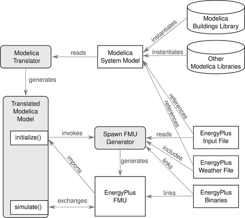
Next, the Translated Modelica Model imports the EnergyPlus FMU, reads parameter values such as the room volume that is computed by EnergyPlus and needed for the Modelica room air heat balance, and then proceeds to the simulation phase. During the simulation phase, data is exchanged at each EnergyPlus zone time step. We refer the reader to the Appendix for a more detailed discussion of each step.

4.3. Translation and simulation

Since version 9.0.0, the Modelica Buildings Library contains all software required to construct a complete Spawn-based building energy model. All software is bundled with the Modelica Buildings Library in a way that is compliant with the Modelica Language Specification. This means that users of Modelica who have installed one of the commercial or open source Modelica environments are able to use the Modelica Buildings Library as any other Modelica library and begin translating and simulating Spawn-based building simulations using their chosen Modelica environment.

5. There is no free lunch

While the coupled simulation introduces new capabilities, it also introduces limitations that are not present in Modelica-only and EnergyPlus-only workflows.

Modelica-only workflows have the advantage that error control is automatic (users don't need to decide when to time sample the envelope), events in the envelope model (such as from schedules or shading device operation) are properly handled even if they don't coincide with a synchronization time step, and no spurious discontinuities are injected into a control loop due to time sampling (such as in Example 6.1 in which a filter had to be added to avoid oscillations in control caused by the discrete time envelope model). Moreover, a Modelica-only simulation allows resetting state variables and obtaining derivatives as needed for model predictive control, linearizing a model around an operating point for controls design, and computing adjoint derivatives using automatic differentiation with back propagation, which is supported via the FMI 3.0 Standard and which is at the heart of many artificial intelligence frameworks and efficient parameter estimation techniques (Baydin et al. 2018).

EnergyPlus-only workflows have several advantages as well. HVAC auto-sizing and report generation can be used. For use cases where load-based HVAC simulation with idealized control suffices – this includes most traditional energy modelling use cases such as architectural design assistance, code compliance calculations and building-stock level evaluation of energy efficiency measures – computing time is generally shorter. Those applications also have established end-to-end tool chains including the OpenStudio SDK for workflow automation and a number of end-user applications and services.

In general, working with a single tool and a single environment is more convenient and smoother than working in multiple tools and environments. Setup, debugging and post-processing are easier. Getting help and support is easier, especially for problems that would exist in the interface between multiple tools.

While Spawn enables models that combine complex geometry, lighting and shading, with novel HVAC systems and realistic control that are not possible to simulate in EnergyPlus or Modelica alone, it also introduces complexity that is inherent in any co-simulation. For example, one has to select how frequent to synchronize models to maintain accuracy and stability. In Spawn, this is done via the EnergyPlus TimeStep object. Also, variables that are sent from one simulator to another are typically not smooth, which may require additional measures to have a continuous changing signal. In the example of Section 6.1, this is done by adding a first-order filter for the room radiative temperature upstream of the PI controller. Moreover, with Spawn, saving and restoring the state of a simulation, as would be needed for model predictive control, is not possible. However, for this use case, the use of a differentiable and simpler envelope model may be favourable, in particular if model parameters are updated during building operation (Blum et al. 2019).

6. Examples

We now present a few examples that illustrate how coupled simulation is achieved with Spawn. For a more comprehensive list of examples that illustrate each feature, we refer the reader to the user guide Buildings.ThermalZones.EnergyPlus_9_6_0.UsersGuide in the Modelica Buildings Library.

6.1. Geothermal heat pump with radiant floor

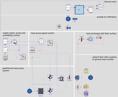
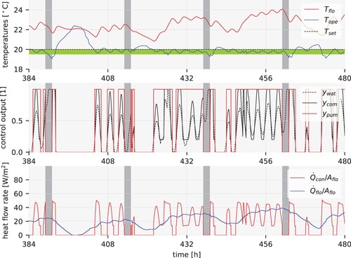
Figure 4 shows a model of a geothermal heat pump system, with a radiant floor slab, that connects to an EnergyPlus thermal zone model and to its floor surface. The model illustrates how to connect Modelica with EnergyPlus. The top of the figure is a Modelica ThermalZone that connects to an EnergyPlus Zone. To its right is a block that computes the operative room temperature using the room air temperature from Modelica and the zone radiative temperature from EnergyPlus. The radiative temperature is fed through a first-order filter because otherwise it would have a discrete jump at every EnergyPlus time step, and this jump would be propagated through the controller, yielding jumps in its output. Immediately below, the thermal zone is connected to a model that provides a constant infiltration mass flow rate and a flow path for exhaust air. The infiltration model is connected to an instance of the Building model, from which it receives the weather data that are used to set the air temperature and humidity (more detailed models for wind-pressure driven infiltration could be used from the Buildings.Airflow.Multizone package, see Wetter 2006). At the bottom left is a geothermal heat pump system. It consists of a water loop that serves the radiant slab and a glycol loop that connects the heat pump to a borehole model. The heat pump is a variable speed model with scroll compressor (Cimmino and Wetter 2017). The heat pump system is controlled using a cascading controller: The first controller closes the outer feedback loop on the room air temperature and outputs a set point temperature for the water that leaves the slab. It also controls the heat pump system on/off. The second controller closes the inner feedback loop on the water temperature leaving the slab, which is compared to this set point. This controller regulates compressor speed. On the bottom right is the radiant slab model, which is connected at the bottom to a model for transient heat conduction in the soil. The top of the radiant slab is connected to a temperature sensor, which feeds the surface temperature to an instance of ZoneSurface. This in turn sets the temperature of an EnergyPlus BuildingSurface:Detailed object and returns its surface heat flow rate, which is then connected to a prescribed heat flow element that connects to the top of the radiant slab.

Figure 4. Model of a thermal zone with infiltration and radiant floor, coupled to a geothermal heat pump.

The top of Figure 5 shows a 5-day period of the floor surface temperature $T_{\mathrm{flo}}$, the zone operative temperature $T_{\mathrm{ope}}$ and its set point $T_{\mathrm{set}}$. The green box indicates the region of the proportional band of the outer controller, which has a gain of $K_p=2{\mathrm{K}}^{-1}$. The dark grey boxes show periods during which the heat pump system is off, e.g. to reduce power consumption during early morning hours when electricity is expensive or carbon intensive. The middle figure shows the control signals. The first cascading controller outputs $y_{\mathrm{wat}}$ to reset the set point for the water temperature that leaves the slab, the second cascading controller outputs $y_{\mathrm{com}}$ to control the compressor speed. Also shown is the on/off signal $y_{\mathrm{pum}}$ for the pumps. The bottom figure shows the heat flux at the heat pump condenser, normalized by the zone's floor area ${\dot{Q}}_{\mathrm{con}}/A_{\mathrm{flo}}$, and the heat flux leaving the room-side facing surface ${\dot{Q}}_{\mathrm{flo}}/A_{\mathrm{flo}}$.

Figure 5. Temperatures, control signals and normalized heat flow rates of radiant slab model. The green rectangle shows the proportional band of the outer controller that regulates the room operative temperature, and the dark grey rectangles show periods when the heat pump system is off.

6.2. Smart thermostat control

NREL and LBNL are currently developing a new method, using Spawn simulations, to evaluate the equipment runtime savings provided by residential smart thermostat algorithms. The current industry method for thermostat evaluation is based on gathering field data from homes where a particular thermostat model is installed and then performing an analysis based on the heating and cooling equipment runtime and room temperature set points. With this, it is difficult to evaluate counterfactuals and therefore to directly compare the performance of different thermostat models with different HVAC equipment. Spawn simulations can be used to evaluate these alternative scenarios, such as how a particular smart thermostat model performs relative to a conventional thermostat with a fixed room temperature set point, and can make these comparisons directly. The research effort is particularly interested in how thermostats perform in conjunction with new generations of HVAC equipment such as variable speed heat pumps, which do not yet have enough representation in the field data to support statistical analysis. The ability to evaluate counterfactual scenarios and make direct comparisons is a key strength of the simulation approach.

Some real-world control algorithms and devices presented a challenge for traditional simulation engines like EnergyPlus. In the case of room temperature thermostats, the specific challenge is that EnergyPlus does not resolve realistic equipment on/off events, instead it models a runtime fraction, which is an estimate for the percentage of time the equipment is running during a simulation time step. This approach was developed when limits in computer power dictated time steps on the order of one hour. While today's computing power is greater and EnergyPlus supports time steps as small as 1 minute, the fundamental approach based on the runtime fraction is still used. In contrast, Spawn simulations naturally capture realistic equipment cycling events, allowing it to be readily coupled with real-world room temperature thermostat algorithms, and if desired even physical room temperature thermostat devices.

The objective of the thermostat study is to evaluate the impact of smart thermostats across the United States using simulation at a statistically relevant scale. To accomplish this, several DOE simulation technologies were combined. First, a sample of EnergyPlus models representing the US residential building stock was obtained from the End Use Load Profiles dataset (Wilson et al. 2022). Second, the EnergyPlus models were reformulated into Spawn models by replacing the HVAC and control components with Modelica-based alternatives. The Modelica HVAC model captures realistic equipment cycling and operation sequences that is critical to the study. Next, the Spawn-based ResStock derivative models are compiled into FMUs that are compatible with BOPTEST, a test harness for building control algorithms (Blum et al. 2021). BOPTEST is used to orchestrate a large-scale test of a particular thermostat algorithm deployed across the sample of building models and the result is a set of key performance indicators which quantify the thermostat performance. The hybrid approach implemented by Spawn leverages a large part of the existing DOE investment in EnergyPlus-based modelling and specifically ResStock, which provides a statistical foundation for the study.

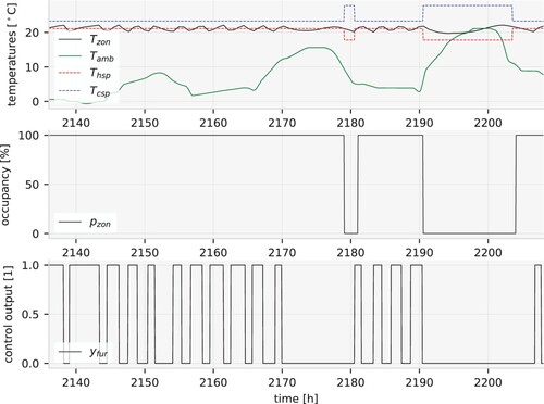
Figure 6 shows one of the HVAC configurations from the thermostat experiment and illustrates how only a few component models from the Modelica Buildings Library can be used to model a typical residential HVAC system coupled to an EnergyPlus based residential building envelope. As in previous examples, Building and Zone models are used to interface with the EnergyPlus building and zone. On the HVAC side, there is a fan, a furnace and an air conditioner model connected together to form a conventional residential single speed DX cooling system with a gas furnace. A custom Modelica thermostat model is used for model development and testing, but during BOPTEST testing the thermostat control signal is overwritten by an external control algorithm of a smart thermostat. A sample of the simulation output is shown in Figure 7, which illustrates the ability of Spawn to capture realistic furnace and air conditioning cycling. The figure shows a 3-day period of time during the shoulder season for which time the thermostat operates in heating mode. In this case, a simulation of an occupancy sensing thermostat is shown, demonstrating how a thermostat could relax the heating and cooling set points during unoccupied periods of time in an effort to reduce equipment runtime. The temperature traces shown in the figure also illustrate the ability of Spawn to capture realistic equipment cycling.

Figure 6. Model of a residential home with a conventional furnace and thermostat control.

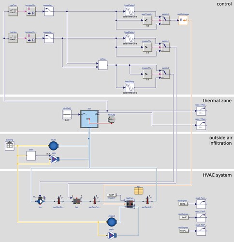
Figure 7. Simulation output for a residential home during a 3-day period in March. The solid black line $T_{\mathrm{zon}}$ shows the effects of realistic equipment cycling within the deadband of the heating set point $T_{\mathrm{hsp}}$. The furnace heating status $y_{\mathrm{fur}}$ correlates with the fluctuating zone temperature. During the two unoccupied periods shown by $p_{\mathrm{zon}}$, the heating and cooling set points $T_{\mathrm{hsp}}$ and $T_{\mathrm{csp}}$ are relaxed.

6.3. Larger examples

Spawn has been used on larger models that are more typical of real-world projects.

Zhang et al. (2022) used Spawn to estimate the energy savings achieved by an ASHRAE Guideline 36 control sequence for a variable air volume flow system in an office building with 21 thermal zones. Wetter, Benne, and Ravache (2021) show that for a building with 50 thermal zones that are served by 10 variable air volume systems that are each controlled with an ASHRAE Guideline 36 control sequence, the models that use the EnergyPlus envelope model rather than the detailed native Modelica envelope model (Wetter, Zuo, and Nouidui 2011) translate about 35% faster and simulate about twice as fast. Gautier, Wetter, and Sulzer (2022) used Spawn to study resilient district energy systems. The authors used high-fidelity, coupled dynamic models of a district energy system with geothermal borefield, energy transfer stations with heat recovery chiller, and building-side HVAC and realistic control logic implemented in Modelica, coupled to an EnergyPlus model of a 2004 vintage multi-zone office building in Chicago, IL. The authors use the coupled simulation to assess different sizing, hydraulic configurations and resulting energy performance and overheating risk during a heat wave in which the geothermal borefield is used to provide cooling without running a vapour compression cycle. Granderson et al. (2022) used Spawn to create data sets that can be used to evaluate and benchmark the performance accuracy of Fault Detection and Diagnostics algorithms. Dey et al. (2023) used Spawn to create control time series data for reinforcement learning building control algorithms that use imitation learning.

7. Conclusion

Spawn couples EnergyPlus envelope modelling with Modelica HVAC and control modelling. The former provide scalable envelope and lighting simulation as well as the ability to use existing envelope model authoring tools. The latter provides the flexibility that the object-oriented, acausal, graphical modelling of Modelica provides for building and district energy and control systems, and the ability to simulate physically-realistic control which can then be directly reused in control implementation workflows.

Spawn works with any Modelica-compliant model authoring and simulation environment. It allows Modelica HVAC system models to be coupled to one or multiple EnergyPlus building envelope models. This composition does not require the user to manually configure a co-simulation setup using either a co-simulation middleware or FMU import and export. Spawn coupling is implemented via the heat exchange between room air which is time-integrated in Modelica, and the comparatively slower changing surface temperatures which are time-integrated in EnergyPlus. This design choice allows for larger coupling time steps in comparison to interfacing to the EnergyPlus room air model as was done in previous couplings. These larger coupling time steps reduce simulation time, in particular for adaptive time step solvers, a family of solvers that are customarily used to simulate stiff systems with continuous and discrete time dynamics as they arise when modelling energy and control systems of buildings and districts.

Disclosure statement

No potential conflict of interest was reported by the author(s).

Data availability

Spawn can be downloaded as part of the Modelica Buildings Library version 8.0.0 or later at simulationresearch.lbl.gov/modelica/download.html. The model used in Section 6.1 is available as ThermalZones.EnergyPlus_9_6_0. Examples.SingleFamilyHouse.HeatPumpRadiantHeatingGroundHeatTransfer in the Modelica Buildings Library at https://github.com/lbl-srg/modelica-buildings/tree/d0040e5. The model used in Section 6.2 cannot be shared publicly.

Additional information

Funding

This research was supported by the Assistant Secretary for Energy Efficiency and Renewable Energy, Office of Building Technologies of the U.S. Department of Energy, under Contracts No. DE-AC02-05CH11231 and DE-AC36-08GO28308. This work emerged from the IBPSA Project 1, an international project conducted under the umbrella of the International Building Performance Simulation Association (IBPSA). Project 1 will develop and demonstrate a BIM/GIS and Modelica Framework for building and community energy system design and operation.

Notes

1 In Modelica, models can be interfaced through connectors which contain all physical properties needed to couple other models. For example, a fluidPort connector contains pressure, mass flow rate, and specific enthalpy, mass fraction and chemical substance concentration carried by the fluid that flows through the connector, whereas a heatPort connector contains temperature and heat flow rate.

2 In Modelica, the thermodynamic behaviour of media, such as air or water, are calculated using a medium model that provides the equation of state (Casella et al. 2006).

3 Note that in contrast to the EnergyPlus Construction object which defines the materials and layer assembly of a construction, the Modelica Buildings Library OpaqueConstruction is a model that represents the physical behaviour of a particular instance of a construction.

4 While the time step length could be read during the getParameters(ptr) step, it is read at each synchronization time step. This allows in the future the use of variable synchronization time steps, for example if EnergyPlus has a change in a schedule or if it exhibits a fast transient that would warrant a shorter synchronization time step.

5 The Spawn FMU generator automatically removes the HVAC and control related EnergyPlus input objects that are not used in a Spawn simulation and retains the input objects that pertain to the building envelope and internal loads. As a non-exhaustive high level summary, input data objects with the following prefixes are supported: Site, Schedule, Material, WindowMaterial, MaterialProperty, Construction, Shading, SurfacePro-perty, GroundHeatTransfer, Daylighting, People, Lights, ElectricEquipment, GasEquip-ment, HotWaterEquipment, SteamEquipment, OtherEquipment, Zone, and ZoneCapacitanceMultiplier. The resulting IDF file that is simulated by Spawn is available for user inspection in the FMU.

6 See, for example, the model Buildings.ThermalZones.EnergyPlus_9_6_0.Validation.Schedule.EquipmentScheduleOutputVariable.

Appendices

This appendix explains the tool coupling, synchronization, and implementation of Spawn in more detail. While deep understanding of these design principles is not necessary for day-to-day use of Spawn, they are included here because many can be applied to other modular co-simulation applications. For example, the execution sequence in Figure A1 and the synchronization mechanism of Algorithm 1 can be applied to other co-simulations in which different Modelica models need to connect to a domain-specific simulator. Examples of such co-simulations include coupling multiple geothermal boreholes, or multiple wells of an aquifer thermal energy storage system, to a subsurface simulator and coupling multiple buildings to an electrical distribution network simulator.

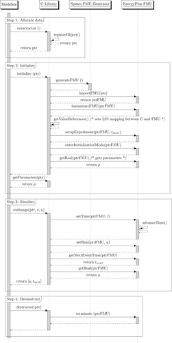
Figure A1. Sequence diagram for generating and interacting between the translated Modelica model, the C Library, the Spawn FMU Generator and the EnergyPlus FMU. This sequence is executed for every building model, e.g. the pointer ptr points to a specific EnergyPlus instance. For example, if a district energy model has five EnergyPlus buildings, there are five distinct pointers ptr.

Appendix 1.

Integrating Modelica and EnergyPlus

This section provides a detailed explanation for how Modelica and EnergyPlus are interfaced. The explanations are based on the flow diagram shown in Figure 3. We assume that we have a Modelica system model that contains one or several models that interact with EnergyPlus, e.g. a ThermalZone and an OutputVariable. We will refer to such models that exchange data between Modelica and EnergyPlus as ME models. Other models from the Modelica Buildings Library and possibly other Modelica libraries may also be present. To simplify the discussion, we assume one EnergyPlus model that is coupled to Modelica. When there are multiple EnergyPlus models, the process is replicated for each one.

When a Modelica translator translates the Modelica model, it creates an executable or an FMU. This translated Modelica model does not contain the EnergyPlus FMU. Next, this translated Modelica model is executed. The execution consists of four main steps as shown in the UML sequence diagram in Figure A1. These steps are as follows:

Step 1: The first step allocates all objects for all ME models, e.g. the models that require data exchange between the translated Modelica model and the EnergyPlus FMU. These data are allocated for every building that is declared in the Modelica model. To manage these data, we implemented within the Modelica Buildings Library a C library with functions that collect information from all Modelica models that need to exchange data with EnergyPlus, and that will configure EnergyPlus, launch the run-time coupling, synchronize the data, and terminate the run-time coupling.

Step 2: The second step is the initialization, during which the translated Modelica model invokes functions in the C library that generate one EnergyPlus FMU for the particular building. The C library then imports the EnergyPlus FMU and instantiates it. This import, as well as any other calls to the EnergyPlus FMU, is done using the FMI Library (Modelon 2022), which is not shown in the figure. The FMI Library is an open-source library that provides high-level C methods to interact with FMUs,

In FMI, the variables of the FMU are accessed via so-called value references, which are integers that point to the respective parameter, input or output variable. In the next step, the C library sets up these value references to configure the I/O mapping. Next, the C library sends to the EnergyPlus FMU the start time of the simulation, and tells the EnergyPlus FMU to enter its initialization mode, and then requests from the EnergyPlus FMU parameter values, such as the volumes of the thermal zones. This volume is then used, for example, in the room air heat and mass balance in Modelica.

Step 3: The third step is the simulation over the time period specified in the translated Modelica model. In this step, the translated Modelica model calls an exchange function in the C library. The C library then sets the current time t in the EnergyPlus FMU, and EnergyPlus simulates until it reaches time t. Next, the C library sets in the EnergyPlus FMU the inputs for time t. The C library then asks from the EnergyPlus FMU how far it can simulate until it reaches the next event, which typically is the next EnergyPlus zone time step, as specified by the EnergyPlus TimeStep object.⁴ Finally, the C library reads the outputs at time t from the EnergyPlus FMU and returns them to the translated Modelica model, together with the next synchronization time $t_{\mathrm{next}}$.

Step 4: Lastly, the fourth step is the destructor step, during which a termination signal is sent to the FMUs. This allows the EnergyPlus FMU to write its output file and shut down the simulation. In this step, the dynamic link library of the imported FMU is unloaded and memory is released.

Appendix 2.

EnergyPlus FMU generation

This section explains how the Spawn FMU Generator that is shown in Figure 3 produces an FMU that encapsulates a single EnergyPlus model and a custom EnergyPlus-based runtime library. The generator console program, spawn, is invoked by the external C library described in Section A. The spawn FMU generator takes as input the JSON file that is generated automatically by Modelica. This JSON file contains the name of the IDF, weather data file and it defines the I/O values required by the corresponding ME models. Given this JSON input file, the Spawn FMU Generator performs the following steps:

1. Modify the user provided IDF for compatibility with Spawn

   1. Remove all infiltration, HVAC and control related input objects ⁵

   2. Configure the SimulationControl input for a single annual run period

   3. Add output variable objects to support the output requested by Modelica

2. Create the FMU directory structure

3. Copy the modified IDF, the specified weather data file, and the EnergyPlus IDD file into the resources sub directory

4. Copy a custom EnergyPlus runtime library, epfmi, into the binary subdirectory

5. Create a modelDescription.xml file according to the FMI specification. This file specifies the I/O of the generated FMU and will be read by Modelica when loading the FMU

6. Compress the FMU directory into a zip file.

Appendix 3.

Modelica–EnergyPlus synchronization

This section explains how the synchronization between the translated Modelica model, the C library and the EnergyPlus FMU is implemented. The explanation is split into the processes that occur during initialization and the processes that occur during the time steps.

Initialization. A key challenge is collecting data from ME models that are needed to construct the EnergyPlus FMU. This data must be collected from Modelica models and sent to the Spawn FMU Generator before any ME model requests a parameter from the C library, e.g. the air volume of a thermal zone.

To implement this, we selected a modular design that allows ME models to be distributed across different models and model hierarchy levels. This way, the user can structure the Modelica system model hierarchy in a modular way that best fits the purpose. This modular design allows, for example, to instantiate a Modelica model $m_1$ that has all thermal zones of a floor, and another Modelica model $m_2$ of the HVAC system that may read an EnergyPlus output to retrieve the occupancy schedule value, and then connect $m_1$ and $m_2$ to form a coupled model. This modular design requires that each component model registers itself in the C library, and these registrations must happen before any ME model requests a parameter value from the EnergyPlus FMU.

In Modelica, registering instances in C can be accomplished by using a Modelica ExternalObject, which is a special class that allows implementing C functions that need to preserve data between subsequent calls. (See Modelica Language Specification 3.5, Sec. 12.9.7 Modelica Association 2021.) The ExternalObject contains a constructor function that is invoked during the model initialization. In view of these objects, the implementation difficulty was to enforce that all constructor functions are called before any ME model requests a parameter value. The reason is that parameter values can – of course – only be requested after the EnergyPlus FMU is generated and loaded, and the FMU can only be generated after all constructor functions tell the C library what objects need to interact with the EnergyPlus FMU. However, the Modelica Language Specification 3.5 does not guarantee that all constructors in a model are called before any Modelica function that uses a return value of a constructor, which is needed to retrieve a parameter value, is being used. In early research code, some Modelica tools invoked the function that requests parameter values from the EnergyPlus FMU before all instances called their constructor. As a consequence, the C library prematurely requested the generation of an (incomplete) FMU, which led to a simulation error. Therefore, we changed the Modelica implementation to enforce the execution sequence shown in Algorithm 1. In view of Algorithm 1, the key challenge is to ensure that Step 1 is completed before Step 2 begins. To enforce this calling sequence, we synchronized all objects using a connector that uses a potential and flow variable, together with inner and outer constructs that hide this complexity from the user. Our implementation is based on the code provided by Beutlich (2021), which was motivated by Elmqvist et al. (2015). Fortunately, this implementation can be done inside the Modelica library, and therefore a user need not setup anything special. The ordering of the constructors and the initialize calls is done automatically. For a minimum representative example that implements this algorithm, we refer the reader to Listings 1 to 9 in Wetter, Benne, and Ravache (2021).

Time steps. For data synchronization during time integration, there are two types of ME models.

1. ME models that only send data from Modelica to EnergyPlus (Actuator and Schedule) do so whenever their input changes. Internal EnergyPlus state is updated by calling ‘Manager’ functions such as EnergyPlus::ScheduleManager::UpdateScheduleValues that are available via the EnergyPlus API.

2. ME models that send input and read output from EnergyPlus (ThermalZone, OpaqueConstruction and ZoneSurface) or that only read output from EnergyPlus (OutputVariable) exchange data whenever EnergyPlus requests a synchronization time step. In version 9.0.0 of the Modelica Buildings Library, this is at the EnergyPlus zone time step.

To implement ‘direct feed-through’ behaviour in which the requested EnergyPlus output changes instantaneously whenever its input changes, the output from an Actuator and Schedule is connected to the input of OutputVariable. While the ME model OutputVariable does not use the value of this input, adding this input will cause Modelica tools to generate the simulation code in a way that first exchanges data with the Actuator or Schedule, and afterwards with the OutputVariable. This allows, for example, setting a plug-load schedule in EnergyPlus from Modelica, using that Schedule to switch on electrical equipment EnergyPlus, and then reading the resulting power use in Modelica using OutputVariable.⁶

Appendix 4.

Implementation of EnergyPlus FMI interface

This section explains changes that were made to EnergyPlus to implement the runtime interface. EnergyPlus has an External Interface feature that enables inter-process data exchange on a time step basis, but this feature does not provide the granular access to EnergyPlus needed by Spawn. It also uses TCP socket communication which adds overhead. To support Spawn, EnergyPlus was refactored to allow more granular simulation control and data exchange with lower overhead. In lieu of sockets, a C++ API that relies on direct memory access was added. The new API provides functions to advance the simulation in time, to set inputs and read outputs within each time step, and to bypass the HVAC and control simulation algorithms, allowing EnergyPlus to be used strictly as a heat balance and daylight calculation engine. The API executes on a separate thread from EnergyPlus, with blocking at key points to manage simulation advance, allowing the latter to execute much as it always has. This modified version of EnergyPlus is compiled into the EnergyPlus runtime library epfmi, which has an API for external calls.

References

- Åkesson, J., K. E. Årzén, M. Gäfvert, T. Bergdahl, and H. Tummescheit. 2010. “Modeling and Optimization with Optimica and JModelica.org – Languages and Tools for Solving Large-scale Dynamic Optimization Problem.” Computers and Chemical Engineering 34 (11): 1737–1749. https://doi.org/10.1016/j.compchemeng.2009.11.011.
- Baetens, R., R. De Coninck, J. Van Roy, B. Verbruggen, J. Driesen, L. Helsen, and D. Saelens. 2012. “Assessing Electrical Bottlenecks At Feeder Level for Residential Net Zero-energy Buildings by Integrated System Simulation.” Applied Energy 96:74–83. https://doi.org/10.1016/j.apenergy.2011.12.098.
- Baudette, M., M. Castro, T. Rabuzin, J. Lavenius, T. Bogodorova, and L. Vanfretti. 2018. “Openipsl: Open-instance Power System Library – Update 1.5 to “iTesla Power Systems Library (IPSL): A Modelica Library for Phasor Time-domain Simulations”.” SoftwareX 7:34–36. https://doi.org/10.1016/j.softx.2018.01.002.
- Baydin, A. G., B. A. Pearlmutter, A. A. Radul, and J. M. Siskind. 2018. “Automatic Differentiation in Machine Learning: a Survey.” Journal of Machine Learning Research 18:1–43.
- Beausoleil-Morrison, I., M. Kummert, F. Macdonald, R. Jost, T. McDowell, and A. Ferguson. 2012. “Demonstration of the New ESP-r and TRNSYS Co-simulator for Modelling Solar Buildings.” Energy Procedia 30:505–514. https://doi.org/10.1016/j.egypro.2012.11.060.
- Beutlich, T. 2021. “Modelica Specification Issue 2842.” https://github.com/modelica/ModelicaSpecification/issues/2842#issuecomment-776194950.
- Blochwitz, T., M. Otter, J. Akesson, M. Arnold, C. Clauß, H. Elmqvist, M. Friedrich, et al. 2012. “The Functional Mockup Interface 2.0: The Standard for Tool Independent Exchange of Simulation Models.” In Proceedings of the 9-th International Modelica Conference, Munich, Germany: Modelica Association. https://doi.org/10.3384/ecp12076173
- Blum, D., K. Arendt, L. Rivalin, M. Piette, M. Wetter, and C. Veje. 2019. “Practical Factors of Envelope Model Setup and Their Effects on the Performance of Model Predictive Control for Building Heating, Ventilating, and Air Conditioning Systems.” Applied Energy 236:410–425. https://doi.org/10.1016/j.apenergy.2018.11.093.
- Blum, D., J. Arroyo, S. Huang, J. Drgoňa, F. Jorissen, H. T. Walnum, Y. Chen, et al. 2021. “Building Optimization Testing Framework (BOPTEST) for Simulation-based Benchmarking of Control Strategies in Buildings.” Journal of Building Performance Simulation 14 (5): 586–610. https://doi.org/10.1080/19401493.2021.1986574.
- Bonvini, M., M. Wetter, and T. S. Nouidui. 2014. “A Modelica Package for Building-To-Electrical Grid Integration.” In 5th BauSim Conference, 6–13. Aachen, Germany: IBPSA-Germany. https://simulationresearch.lbl.gov/wetter/download/2014-BauSim-BonviniWetterNouidui.pdf.
- Bortoff, S. A., P. Schwerdtner, C. Danielson, S. D. Cairano, and D. J. Burns. 2022. “H-infinity Loop-shaped Model Predictive Control with HVAC Application.” IEEE Transactions on Control Systems Technology 30:2188–2203. https://doi.org/10.1109/TCST.2022.3141937.
- Casella, F., and A. Leva. 2003. “Modelica Open Library for Power Plant Simulation: Design and Experimental Validation.” In Proceedings of the 3rd Modelica Conference, edited by P. Fritzson, 41–50. Linköping, Sweden: Modelica Association and Institutionen för datavetenskap, Linköpings universitet. https://modelica.org/events/Conference2003/papers/h08_Leva.pdf.
- Casella, F., M. Otter, K. Proelss, C. Richter, and H. Tummescheit. 2006. “The Modelica Fluid and Media Library for Modeling of Incompressible and Compressible Thermo-Fluid Pipe Networks.” In Proceedings of the 5-th International Modelica Conference, edited by C. Kral and A. Haumer, 631–640. Vienna, Austria: Modelica Association and Arsenal Research. http://www.modelica.org/events/modelica2006/Proceedings/sessions/Session6b1.pdf.
- Cimmino, M., and M. Wetter. 2017. “Modelling of Heat Pumps with Calibrated Parameters Based on Manufacturer Data.” In Proceedings of the 12-th International Modelica Conference, 219–226. Prague, Czech Republic: Modelica Association. https://doi.org/10.3384/ecp17132219.
- Crawley, D. B., L. K. Lawrie, F. C. Winkelmann, W. F. Buhl, Y. J. Huang, C. O. Pedersen, R. K. Strand, et al. 2001. “EnergyPlus: Creating a New-generation Building Energy Simulation Program.” Energy and Buildings 33 (4): 319–331. https://doi.org/10.1016/S0378-7788(00)00114-6.
- Dey, S., T. Marzullo, X. Zhang, and G. Henze. 2023. “Reinforcement Learning Building Control Approach Harnessing Imitation Learning.” Energy and AI 14:100255. https://doi.org/10.1016/j.egyai.2023.100255.
- Dietl, K., S. G. Yances, A. Johnsson, J. Åkesson, K. Link, and S. Velut. 2014. “Industrial Application of Optimization with Modelica and Optimica Using Intelligent Python Scripting.” In 10-th International Modelica Conference, 777–786. Lund, Sweden: Modelica Association.
- Dols, W. S., S. J. Emmerich, and B. J. Polidoro. 2016. “Using Coupled Energy, Airflow and Indoor Air Quality Software (TRNSYS/CONTAM) to Evaluate Building Ventilation Strategies.” Building Services Engineering Research and Technology 37 (2): 163–175. https://doi.org/10.1177/0143624415619464.
- Doughty, C., J. Hu, P. Dobson, P. Nico, and M. Wetter. 2021. “Coupling Subsurface and Above-Surface Models for Optimizing the Design of Borefields and District Heating and Cooling Systems in the Presence of Varying Water-Table Depth.” In Proceedings of 46th Workshop on Geothermal Reservoir Engineering, Palo Alto, CA, USA, https://simulationresearch.lbl.gov/wetter/download/2021-geoThermal-DoughtyEtAl.pdf.
- Elmqvist, H., A. Goteman, V. Roxling, and T. Ghandriz. 2015. “Generic Modelica Framework for Multibody Contacts and Discrete Element Method.” In 11-th International Modelica Conference, edited by P. Fritzson and H. Elmqvist, 427–440. Paris, France: Modelica Association. https://doi.org/10.3384/ecp15118427.
- Elsheikh, A., M. U. Awais, E. Widl, and P. Palensky. 2013. “Modelica-Enabled Rapid Prototyping of Cyber-Physical Energy Systems via the Functional Mockup Interface.” In Modeling and Simulation of Cyber-Physical Energy Systems (MSCPES), 2013 Workshop on, 1–6. IEEE.
- Elsheikh, A., E. Widl, P. Pensky, F. Dubisch, M. Brychta, D. Basciotti, and W. Müller. 2013. “Modelica-Enabled Rapid Prototyping via TRNSYS.” In The 13th International Conference of the International Building Performance Simulation Association.
- Fritzson, P., A. Pop, K. Abdelhak, A. Ashgar, B. Bachmann, W. Braun, D. Bouskela, et al. 2020. “The OpenModelica Integrated Environment for Modeling, Simulation, and Model-Based Development.” Modeling, Identification and Control: A Norwegian Research Bulletin 41 (4): 241–295. https://doi.org/10.4173/mic.2020.4.1.
- Gautier, A., M. Wetter, and M. Sulzer. 2022. “Resilient Cooling Through Geothermal District Energy System.” Applied Energy 325:119880. https://doi.org/10.1016/j.apenergy.2022.119880.
- Granderson, J., G. Lin, Y. Chen, A. Casillas, P. Im, S. Jung, K. Benne, et al. 2022. “LBNL Fault Detection and Diagnostics Datasets.” Technical Report, Lawrence Berkeley National Laboratory. https://doi.org/10.25984/1881324.
- Hu, J., C. Doughty, P. Dobson, P. Nico, and M. Wetter. 2020. “Coupling Subsurface and Above-Surface Models for Design of Borefields and Geothermal District Heating and Cooling Systems.” In Proceedings of 45th Workshop on Geothermal Reservoir Engineering, Palo Alto, CA, USA. https://simulationresearch.lbl.gov/wetter/download/2020-HuDoughtyEtAl.pdf.
- Jorissen, F., G. Reynders, R. Baetens, D. Picard, D. Saelens, and L. Helsen. 2018. “Implementation and Verification of the IDEAS Building Energy Simulation Library.” Journal of Building Performance Simulation 11 (6): 669–688. https://doi.org/10.1080/19401493.2018.1428361.
- Krammer, M., K. Schuch, C. Kater, K. Alekeish, T. Blochwitz, S. Materne, A. Soppa, and M. Benedikt. 2019. “Standardized Integration of Real-Time and Non-Real-Time Systems: The Distributed Co-Simulation Protocol.” In Proceedings of the 13th International Modelica Conference, 87–96. Regensburg, Germany: Modelica Association. https://doi.org/10.3384/ecp1915787.
- Laferrière, A., M. Cimmino, D. Picard, and L. Helsen. 2020. “Development and Validation of a Full-time-scale Semi-analytical Model for the Short- and Long-term Simulation of Vertical Geothermal Bore Fields.” Geothermics 86:101788. https://doi.org/10.1016/j.geothermics.2019.101788.
- LBNL. 2013. “FMU Export of EnergyPlus.” https://simulationresearch.lbl.gov/fmu/EnergyPlus/export/index.html.manual.
- Lenord, O., M. Otter, C. Bürger, M. Hussmann, P. L. Bihan, J. Niere, A. Pfeiffer, R. Reicherdt, and K. Werther. 2021. “eFMI: An Open Standard for Physical Models in Embedded Software.” In Proceedings of the 14th International Modelica Conference, edited by M. Sjölund, L. Buffoni, A. Pop and L. Ochel, 57–71. Modelica Association and Linköping University Electronic Press. https://doi.org/10.3384/ecp2118157.
- Maccarini, A., M. Wetter, A. Afshari, G. Hultmark, N. C. Bergsøe, and A. Vorre. 2017. “Energy Saving Potential of a Two-pipe System for Simultaneous Heating and Cooling of Office Buildings.” Energy and Buildings 134:234–247. https://doi.org/10.1016/j.enbuild.2016.10.051.
- MacRae, N., J. Batteh, S. Velut, W. Skravin, I. Khan, and D. Jang. 2020. “Micro-Grid Design and Cost Optimization Using Modelica.” In 2nd American Modelica Conference, Boulder, CO, USA. https://doi.org/10.3384/ecp2016918.
- Mattsson, S. E., M. Otter, and H. Elmqvist. 1999. “Modelica Hybrid Modeling and Efficient Simulation.” In 38th IEEE Conference on Decision and Control, 3502–3507. Phoenix, AZ: IEEE. http://www.modelica.org/publications/papers/ModelicaCDC99.pdf.
- Modelica Association. 2019. “System Structure and Parameterization.” Technical Report. https://ssp-standard.org/.
- Modelica Association. 2021. “Modelica Language Specification 3.5.” Accessed February 07, 2023. https://specification.modelica.org/maint/3.5/MLS.html.
- Modelon. 2022. “FMI Library.” Accessed November 21, 2022. https://github.com/modelon-community/fmi-library.
- Müller, D., M. Lauster, A. Constantin, M. Fuchs, and P. Remmen. 2016. “Aixlib – An Open-Source Modelica Library Within the IEA-EBC Annex 60 Framework.” In BauSIM 2016. http://www.ibpsa.org/proceedings/bausimPapers/2016/A-02-3.pdf.
- Nouidui, T. S., and M. Wetter. 2014. “Linking Simulation Programs, Advanced Control and FDD Algorithms with a Building Management System Based on the Functional Mock-Up Interface and the Building Automation Java Architecture Standards.” In ASHRAE/IBPSA-USA Building Simulation Conference, 49–55. Atlanta, GA: IBPSA-USA. http://simulationresearch.lbl.gov/wetter/download/2014-IBPSA-USA-NouiduiWetter.pdf.
- Nouidui, T. S., M. Wetter, and W. Zuo. 2014. “Functional Mock-up Unit for Co-simulation Import in EnergyPlus.” Journal of Building Performance Simulation 7 (3): 192–202. https://doi.org/10.1080/19401493.2013.808265.
- Nytsch-Geusen, C., J. Huber, M. Ljubijankic, and J. Rädler. 2013. “Modelica BuildingSystems – Eine Modellbibliothek Zur Simulation Komplexer Energietechnischer Gebäudesysteme.” Bauphysik 35 (1): 21–29. https://doi.org/10.1002/bapi.201310045.
- Pazold, M., S. Burhenne, J. Radon, S. Herkel, and F. Antretter. 2012. “Integration of Modelica Models into an Existing Simulation Software Using FMI for Co-Simulation.” In 9th International Modelica Conference. https://doi.org/10.3384/ecp12076949.
- Pfeiffer, A. 2012. “Optimization Library for Interactive Multi-Criteria Optimization Tasks.” In Proceedings of the 9-th International Modelica Conference, 669–679. Munich, Germany: Modelica Association. https://doi.org/10.3384/ecp12076669.
- Roth, A., M. Wetter, K. Benne, D. Blum, Y. Chen, G. Fierro, M. Pritoni, A. Saha, and D. Vrabie. 2022. “Towards Digital and Performance-Based Supervisory HVAC Control Delivery.” In Proceedings of the ACEEE 2022 Summer Study on Energy Efficiency in Buildings, ACEEE, Asilomar, Pacific Grove, CA, 3.528–3.543. https://simulationresearch.lbl.gov/wetter/download/2022-RothEtAl.pdf.
- Senkel, A., C. Bode, J. P. Heckel, O. Schülting, G. Schmitz, C. Becker, and A. Kather. 2021. “Status of the TransiEnt Library: Transient Simulation of Complex Integrated Energy Systems.” In Proceedings of the 14th International Modelica Conference, edited by M. Sjölund, L. Buffoni, A. Pop and L. Ochel, 187–196. Modelica Association and Linköping University Electronic Press. https://doi.org/10.3384/ecp21181187.
- Sommer, T., M. Sulzer, M. Wetter, A. Sotnikov, S. Mennel, and C. Stettler. 2020. “The Reservoir Network: A New Network Topology for District Heating and Cooling.” Energy 199:117418. https://doi.org/10.1016/j.energy.2020.117418.
- Wetter, M. 2006. “Multizone Airflow Model in Modelica.” In Proceedings of the 5th International Modelica Conference, edited by C. Kral and A. Haumer, 431–440. Vienna, Austria: Modelica Association and Arsenal Research. http://www.modelica.org/events/modelica2006/Proceedings/sessions/Session413.pdf.
- Wetter, M. 2009. “Modelica-based Modeling and Simulation to Support Research and Development in Building Energy and Control Systems.” Journal of Building Performance Simulation 2:143–161. https://doi.org/10.1080/19401490902818259.
- Wetter, M. 2011. “Co-simulation of Building Energy and Control Systems with the Building Controls Virtual Test Bed.” Journal of Building Performance Simulation 4 (3): 185–203. https://doi.org/10.1080/19401493.2010.518631.
- Wetter, M. 2022. “IBPSA Modelica Working Group.” https://github.com/ibpsa/modelica-working-group.
- Wetter, M., K. Benne, and B. Ravache. 2021. “Software Architecture and Implementation of Modelica Buildings Library Coupling for Spawn of EnergyPlus.” In Proceedings of the 14th International Modelica Conference, edited by M. Sjölund, L. Buffoni, A. Pop and L. Ochel, 325–334. Modelica Association and Linköping University Electronic Press. https://doi.org/10.3384/ecp21181325.
- Wetter, M., P. Ehrlich, A. Gautier, M. Grahovac, P. Haves, J. Hu, A. Prakash, D. Robin, and K. Zhang. 2022. “OpenBuildingControl: Digitizing the Control Delivery From Building Energy Modeling to Specification, Implementation and Formal Verification.” Energy 238:121501. https://doi.org/10.1016/j.energy.2021.121501.
- Wetter, M., M. Fuchs, P. Grozman, L. Helsen, F. Jorissen, M. Lauster, D. Müller, et al. 2015. “IEA EBC Annex 60 Modelica Library – An International Collaboration to Develop a Free Open-Source Model Library for Buildings and Community Energy Systems.” In: 14-th IBPSA Conference, 395–402. International Building Performance Simulation Association. http://www.iea-annex60.org/downloads/p2414.pdf.
- Wetter, M., A. Gautier, M. Grahovac, and J. Hu. 2019. “Verification of Control Sequences Within OpenBuildingControl.” In 16-th IBPSA Conference, 885–892. International Building Performance Simulation Association. http://simulationresearch.lbl.gov/wetter/download/2019-ibpsa-OpenBuildingControl.pdf. https://doi.org/10.26868/25222708.2019.210722.
- Wetter, M., M. Grahovac, and J. Hu. 2018. “Control Description Language.” In 1st American Modelica Conference, Cambridge, MA, USA. https://doi.org/10.3384/ecp1815417.
- Wetter, M., and C. van Treeck. 2017. “IEA EBC Annex 60: New Generation Computing Tools for Building and Community Energy Systems.” http://www.iea-annex60.org/pubs.html.
- Wetter, M., C. van Treeck, L. Helsen, A. Maccarini, D. Saelens, D. Robinson, and G. Schweiger. 2019. “IBPSA Project 1: BIM/GIS and Modelica Framework for Building and Community Energy System Design and Operation–ongoing Developments, Lessons Learned and Challenges.” IOP Conference Series: Earth and Environmental Science 323:012114. https://doi.org/10.1088/1755-1315/323/1/012114.
- Wetter, M., W. Zuo, and T. S. Nouidui. 2011. “Modeling of Heat Transfer in Rooms in the Modelica Buildings Library.” In Proceedings of the 12-th IBPSA Conference, 1096–1103. International Building Performance Simulation Association. https://simulationresearch.lbl.gov/wetter/download/2011-ibpsa-BuildingsLib.pdf.
- Wetter, M., W. Zuo, T. S. Nouidui, and X. Pang. 2014. “Modelica Buildings Library.” Journal of Building Performance Simulation 7 (4): 253–270. https://doi.org/10.1080/19401493.2013.765506.
- Wilson, E. J. H., A. Parker, A. Fontanini, E. Present, J. L. Reyna, R. Adhikari, C. Bianchi, et al. 2022. “End-Use Load Profiles for the U.S. Building Stock: Methodology and Results of Model Calibration, Validation, and Uncertainty Quantification.” https://doi.org/10.2172/1854582.
- Zhang, K., D. Blum, H. Cheng, G. Paliaga, M. Wetter, and J. Granderson. 2022. “Estimating ASHRAE Guideline 36 Energy Savings for Multi-zone Variable Air Volume Systems Using Spawn of EnergyPlus.” Journal of Building Performance Simulation 15 (2): 215–236. https://doi.org/10.1080/19401493.2021.2021286.
- Zhang, K., D. H. Blum, M. Grahovac, J. Hu, J. Granderson, and M. Wetter. 2020. “Development and Verification of Control Sequences for Single-Zone Variable Air Volume System Based on ASHRAE Guideline 36.” In 2nd American Modelica Conference, Boulder, CO, USA. https://doi.org/10.3384/ECP2016981.