Toward practical algorithms for activity chain optimization

ABSTRACT

Activity Chain Optimization (ACO) is the task of finding a minimum-cost tour that visits exactly one location for each required activity while respecting time window constraints. We develop an exact algorithm that efficiently solves the ACO problem in all practical cases that involve hundreds of locations offering up to 10–15 activities and returns the optimal route with minimal time spent traveling and waiting. We also introduce a greedy heuristic that simulates human decision-making for comparison. Our experimental results highlight the practical significance of our work as we can reduce travel and wait times on 45 realistic Budapest inner-city routing problems by 16.65% on average compared to our baseline. Our algorithms’ computational and memory requirements for solving practical ACO instances are shown to be low enough to be employed on embedded devices, e.g. smartphones and navigation systems.

KEYWORDS:

• Activity chain optimization
• traveling salesman problem
• combinatorial optimization

Introduction

The field of travel demand modeling and transportation optimization is currently moving toward personalized and activity-based travel behavior analysis (Rasouli and Timmermans 2014). The defining characteristics of our Activity Chain Optimization (ACO) problem formulation – in contrast to the classical route planning tasks – are (1) the spatial flexibility (i.e. interchangeability) of demand points that offer the same activity and (2) the temporal constraints that allow engaging in a certain activity at a given location within given time intervals only. Both characteristics emphasize the need for activity-centered modeling (instead of trip- and route-based models). The simultaneous incorporation of both individually specified and environment-given freedom and restrictions in time and space – governed by the final goal of accomplishing predefined activities with maximum utility – increases the level of realism and thus practical significance.

Most notably, our ACO formulation naturally translates to the common problem of planning an efficient itinerary for everyday commute or making the best use of the available time as a tourist in a foreign location. Other areas of possible practical significance can also be identified, e.g. robotic logistics or manufacturing, where there could be several possible trajectories for performing the same activity while having to obey certain time constraints (Chettibi et al. 2004).

The Activity Chain Optimization problem can be understood as part of the family of Traveling Salesman Problem (TSP) variants. Since TSP can be reduced to ACO by simply setting each location to offer its own unique activity (thus removing interchangeability) while also setting time windows to be all-inclusive (thus effectively removing time windows), it becomes evident that ACO is more general and at least as hard as TSP. Therefore, ACO is also an NP-hard problem, while – along a similar line of reasoning – the decision version of the ACO problem is NP-complete. This means in practical terms that there are no algorithms that are both fast (polynomial-time) and exact (optimal)¹. As in the TSP case, there will always be a problem size up to which exact algorithms are feasible (and even recommended), while above that certain limit only approximation and heuristic methods can prove useful. In this paper, we argue that most human daily activity chains are shorter than 10–15 activities (or can be broken into short sequential subsets) and thus fall into the range that can be efficiently optimized by our proposed exact algorithm – even on embedded devices. Accordingly, we focus on the problem size of 5–9 activities with hundreds of locations for our measurements and show that optimal solution of the problem in realistic scenarios is easily attainable and yields an average improvement of $16.65\pm 4.21\mathrm{\%}$ upon our baseline with $90\mathrm{\%}$ confidence.

Related work

Activity planning methods

Integrated transport policies, analysis of travel-related information and optimization of mobility patterns could be considered fundamental tools in reducing travel time, travel distance and/or other transportation-related costs with the aim of better serving the mobility needs of citizens. This can be realized by introducing intelligent activity planning methods, especially the organization of daily activity chains. One basic work in this field originates from (Timmermans et al. 2003), who described and analyzed travel patterns. In the paper of (Liao, Arentze, and Timmermans 2013) activity-travel scheduling was handled as a modeling problem. Their aim was to provide a model to predict short-term effects of travel information systems and travel demand management. (Sharmeen, Arentze, and Timmermans 2013) analyzed the effects of activities on long-term changes and dynamics of time allocation in activities. (Comi and Nuzzolo 2016) created a new method for generating path advice for multimodal travel networks. The method uses individual traveler utility functions, which allows personal preferences to be included. Maximizing utility on a larger, social scale (Li et al. 2016) formulate the time-dependent activity choice and multimodal travel choice equilibrium problem as a variational inequality problem. They propose a new model for fuel surcharge and transit service runs optimization. A Bayesian network-based modeling approach is considered by Xie and Waller (2010), who give a method for estimating the network structure and thus capturing complex travel choice patterns. (Hafezi, Liu, and Millward 2018) developed a methodology for modeling the daily activity engagement patterns of individuals. The dependencies between activity type, activity frequency, and socio-demographic characteristics are taken into account while employing a Random Forest model. (Hilgert et al. 2016) developed a mobility assistance system which gathers information from timetables and real-time information systems in public transportation, and is also connected to mobility services (e.g. car sharing). Furthermore, it knows the user’s schedule and can reorganize weekly activity schedule according to personal preferences. The organization of the daily activity chains has been analyzed in several articles (Miller and Roorda 2003) and books (Timmermans and Petrus 2005).

In the literature we see that one major approach to activity scheduling is to minimize costs and maximize utility for all traffic participants as an aggregate: such a holistic approach operates from a traffic management and traffic assignment perspective. Dynamic Traffic Assignment (DTA) (Heydecker and Addison 2006) is considered to be a rapidly evolving subfield in this area that is characterized by congestion forecasting models and route assignment equilibration based on experienced travel times, not instantaneous travel times (or other cost/utility measures). Although neither holism nor dynamics modeling are in the focus of our current work, DTA literature significantly expands upon several methodological challenges that arise during activity optimization in general. These challenges include, for example, departure time choice² and time-dependent road pricing (Polak and Heydecker 2006). In this paper, we assume a simple model with fixed departure time and a straightforward instantaneous travel and experienced waiting time-based cost. A problem formulation reminiscent of ours is given by Abdelghany and Mahmassani (2003) who present a DTA method that iteratively refines the departure times, route choices and activity sequences of thousands of commuters. While optimizing for the individual commuter, our method differs also in its capacity: we can handle up to 10–15 activities and can perform these at hundreds of alternative locations, while their method is designed for up to 3 activities at fixed (singular) locations. Others optimize even more complex and more realistic models, e.g. activity duration-dependent and scheduling-dependent utility functions (Cantelmo and Viti 2019). In a prior work, Li, Lam, and Wong (2014) utilize a bottleneck model for congestion and assume constant and linear marginal-activity utility functions. Much of this complexity is necessarily absent from our work in order to facilitate the fast and optimal algorithmic solution we provide. In particular, we model the problem not in terms of relative and often (time-)variable utility of activities, scheduling, departure times, etc., but rather in absolute terms of required activities, possible locations and preferred time windows, which ultimately puts our formulation into the realm of tractable discrete optimization. Altogether, our method does not belong to the family of DTA methods. Nevertheless, we do model certain aspects of variability in travel times and activity duration as indicated throughout Sections 3 and 7.

The other major approach to activity scheduling is more focused on optimizing the individual user’s cost and utility without regards to how it affects other users, and this is the approach that we investigate in our current paper. Many problem models exist for this perspective, but TSP has the widest literature and range of applications (Gutin and Punnen 2002). Our particular ACO problem variant inspired by (Esztergár-Kiss, Rózsa, and Tettamanti 2017) will be defined as a combination of the Generalized TSP (GTSP) and TSP with Time Windows (TSPTW) in Section 3.

Exact solutions to the classical TSP

The origin of the Traveling Salesman Problem goes back to the late 19^th century (Voigt 1831), and the first formal mathematical study of the problem can be traced back to (Menger 1931). Menger defines the problem essentially as finding the minimum weight Hamiltonian cycle in a metric graph, and is intrigued by the question of whether it is possible to devise an algorithm that reduces runtime complexity below the brute force $O(n!)$. Nineteen years later, Julia Robinson at RAND Corporation develops a method for solving the assignment problem (Robinson 1949), which result is then subsequently used by her colleagues in a paper (Dantzig, Fulkerson, and Johnson 1954) that presents the optimal tour solution through 49 US cities. The method of achieving the solution also contributed to the development of the simplex algorithm (Dantzig, Orden, and Wolfe 1955) – one the most popular and useful ways of solving general purpose optimization problems that can be formulated as linear programs. However, the first theoretically sound upper runtime bound for TSP that lies below $O(n!)$ is given only much later by Held and Karp (1962), who present a dynamic programming-based algorithm that runs in $O(2^n{n}^2)$. Up to this day, this remains the best-known running time bound for any algorithm that solves the classical TSP. The Held-Karp dynamic programming approach also forms the basis for the exact solution we present in this paper. Although dynamic programming gives the best runtime guarantees, in practice it is not the fastest method and scales only up to dozens of nodes. Linear programming-based cutting-plane and branch and bound methods can exactly solve much larger instances by approaching the optimum from both primal and dual directions – the largest practical problem solved being an 85,900 node VLSI application (Applegate et al. 2009) – albeit with much looser runtime upper bound guarantees³ (Applegate et al. 2011). Exploring linear programming-based approaches to the ACO problem is a possible next step for our research, but would be motivated by different applications with longer activity chains (maybe industrial robotics, e.g. manufacturing, bin-packing or automated guided vehicle routing as in Fazlollahtabar and Saidi-Mehrabad (2015)). For the optimization of realistic daily commute activity chains of length 5–9 the linear programming approach is ultimately not necessary.

Approximate solutions and heuristics

If the problem size or structure is such that the exact optimum is not efficiently obtainable, approximations and heuristics can be employed. The most important TSP approximation to note is the Christofides algorithm (Christofides 1976), which runs in polynomial time ($O(n^3)$) and guarantees that the obtained solution’s cost will be within $\frac{3}{2}$ of the optimum, but also requires the TSP to be metric (i.e. edge weights have to satisfy the triangle condition). No other polynomial algorithm to date can deliver a tighter bound. The nearest neighbor heuristic, in contrast, only guarantees an upper approximation ratio bound of $1+\frac{logn}{2}$ in the case of metric TSP, and provides no guarantees otherwise (Cook 2012). An even looser bound of $4\sqrt{n}$ is given by the fast-running Lin–Kernighan (LKH) heuristic (Helsgaun 2000) which gradually employs so-called 2-opt, 3-opt and 5-opt improvements and very often produces optimal results in practice (Rego et al. 2011). Other heuristic approaches include large neighborhood searches (Smith and Imeson 2017), simulated annealing (Barach et al. 2012), ant colony optimization (Kona and Burde 2015; Yao et al. 2016; Nadizadeh and Kafash 2019) and genetic algorithms (Grefenstette 1985). (Esztergár-Kiss, Rózsa, and Tettamanti 2018) describe a genetic algorithm approach to the ACO problem.

Problem definition

We can informally describe the ACO problem as follows: given a starting time and location and a map of pairwise times and costs of travel between locations that each offer the possibility for exactly one type of activity within a given time window, and given a list of desired processing durations for each activity type, find the cheapest tour that visits and performs all required activities exactly once and returns to the starting location before a given deadline. A formal definition will be given below.

The ACO problem

Let $\mathcal{G}=(\mathcal{V},\mathcal{E})$ be a directed graph, with location vertices $\mathcal{V}=\{0,1,\dots ,n-1\}$ partitioned into ${\mathcal{A}}_0=\{0\},{\mathcal{A}}_1,\dots ,{\mathcal{A}}_{m-1}$ disjunct non-empty activity clusters. Note that $m\le n$ and $m,n\in {\mathbb{N}}^{+}$. Each directed edge $(i,j)\in \mathcal{E}$ can be mapped to a cost $C_{ij}\in \mathbb{R}$ and a traveling time $T_{ij}\in {\mathbb{R}}_{\ge 0}$ between vertices $i$ and $j$ $(i,j\in \mathcal{V})$. It is both necessary and sufficient to define edges, costs and travel times between vertices belonging to different activity clusters only, i.e. $\mathcal{E}=\{(i,j):i\in {\mathcal{A}}_u,j\in {\mathcal{A}}_v,u\ne v\}$. Each location vertex $j$ is also assigned a time window $W_j=[{w_j}^{\prime },w{{ }^{\prime \prime }}_j]$ where $w^{\prime },w^{\prime \prime }\in {\mathbb{R}}_{\ge 0}$. The task is to find a finite-time minimum cost Hamiltonian cycle starting from and ending at vertex $0$ (corresponding to a unique home activity and location), such that exactly one vertex of each activity cluster is visited and the arrival time ${\hat{t}}_j$ at each visit either falls within the visited node’s time window $W_j$ or precedes it. The recursive relation between ${\hat{t}}_j\in {\mathbb{R}}_{\ge 0}$ arrival times (arrival at node $j$) and $t_j\in {\mathbb{R}}_{\ge 0}$ ready times (ready for departure from node $j$) is as follows:

For a given path described by the sequence of nodes $⟨\dots ,i,j,\dots ⟩$ where $(i,j)\in \mathcal{E}$:

(1) $\begin{array}{cc}{t}_0& \mathrm{i}\mathrm{s}\mathrm{g}\mathrm{i}\mathrm{v}\mathrm{e}\mathrm{n}\\ {\hat{t}}_j& =t_i+T_{ij}\\ t_j& =\left\{\begin{array}{cc}{w}_j^{\prime }& \mathrm{i}\mathrm{f}{\hat{t}}_j<w_j^{\prime }\\ {\hat{t}}_j& \mathrm{i}\mathrm{f}{w}_j^{\prime }\le {\hat{t}}_j\le w_j^{{ }^{\prime \prime }}\\ \mathrm{\infty }& \mathrm{o}\mathrm{t}\mathrm{h}\mathrm{e}\mathrm{r}\mathrm{w}\mathrm{i}\mathrm{s}\mathrm{e}\end{array}\right.\end{array}$(1)

${\hat{t}}_{0^{\prime }}$ and $t_{0^{\prime }}\in {\mathbb{R}}_{\ge 0}$ will denote arrival and ready times when returning to the home vertex (which may also have a time window) at the end of the circuit. Their calculation proceeds with the same recursive logic outlined above. Finding a finite-time solution means $t_{0^{\prime }}<\mathrm{\infty }$.

If the real-world task involves time-consuming activities that have a duration ${\delta }_j\ge 0$ where $j\in \mathcal{V}$ ($\delta$ may or may not be uniform throughout different locations for the same activity), these durations can be represented in the problem model by integrating them into the travel time matrix, i.e. adding them to the preceding travel times obtaining $T_{ij}\leftarrow T_{ij}+{\delta }_j$ for all $(i,j):i,j\in \mathcal{V}$. The time windows should also be adjusted to designate the earliest and latest finishing (ready) times for their respective activity by shifting all $w_j^{\prime }$ values as follows: $w_j^{\prime }\leftarrow w_j^{\prime }+{\delta }_j$.

If the real-world task involves a multi-activity location $i$, it can be represented as a group of separate single-activity locations $i_1,i_2,\dots$ with appropriate intra-group travel times $t_{i_{from},i_{to}}=0+{\delta }_{i_{to}}$. Intra-group costs can be set to zero, or if the travel cost function includes a component unrelated to travel but related to the activity itself, a similar integration can be performed as in the case of travel times and activity durations.

If the real-world task involves performing the same activity more than once (maybe in different locations or time-intervals), then this should be modeled as different activities.

tACO: time-based ACO

We define the time-based Activity Chain Optimization (tACO) problem variant as

• having durations that are uniform throughout different locations for the same activity: $\mathrm{\forall }i,j\in V({\delta }_i={\delta }_j\Leftarrow \mathrm{\exists }u(i,j\in A_u))$, and

• having a dynamic cost function associated with a transition from node $i$ to $j$:

  (2) $C_{ij}(t_i)=max\{T_{ij},w_j^{\prime }-t_i\}$(2)

The goal in the tACO problem variant is to minimize all time spent ‘uselessly’, i.e. to minimize the sum of all time spent traveling and waiting. The total cost function to be minimized therefore will be formulated as follows.

Given a valid solution sequence $s=⟨s_0,s_1,s_2,\dots ,s_{m-1},s_m⟩$ where $m$ is the total number of activities and $s_0=s_m=0$ and for all $i,j\in \{0,\dots ,m-1\}$ $s_i,s_j\in \mathcal{V}$ and when $i\ne j$ then $s_i\in {\mathcal{A}}_u,s_j\in {\mathcal{A}}_v,u\ne v$, furthermore having defined the length of the sequence as $|s|=m+1$, minimize the following recursive objective function:

(3) $\begin{array}{rl}& C(s)=\left\{\begin{array}{cc}{\sum }_{k=1}^{|s|-1}{C}_{k-1,k}\left(C(⟨s_0,\dots ,s_{k-1}⟩)\right)& \mathrm{i}\mathrm{f}|s|>1\\ t_0& \mathrm{o}\mathrm{t}\mathrm{h}\mathrm{e}\mathrm{r}\mathrm{w}\mathrm{i}\mathrm{s}\mathrm{e}\end{array}\right.\\ & \mathrm{w}\mathrm{h}\mathrm{e}\mathrm{r}\mathrm{e}C(⟨0⟩)=t_0\mathrm{i}\mathrm{s}\mathrm{g}\mathrm{i}\mathrm{v}\mathrm{e}\mathrm{n}\end{array}$(3)

We will note that the objective function now contains the sum of all travel times, waiting times, and activity processing times – as the activity durations are already integrated into the travel times matrix and the time windows by definition. Since the durations are uniform for a given activity, and since we know that all activities will be visited exactly once, we understand that the sum of durations ${\sum }_i{\delta }_{s_i}$ in any valid (but not necessarily optimal) sequence $s$ must always be the same. Therefore, the sequence that minimizes the cost function (i.e. the sum of all travel times, waiting times and processing times) will inevitably minimize the ‘uselessly’ spent time (the sum of all travel times and waiting times) as well.

Starting from Section 4 we will focus on the tACO problem exclusively unless noted otherwise, as the main contributions outlined in this paper lie in developing algorithms for this problem variant.

Developed algorithms

In the following, we present the detailed description and asymptotic complexity analysis of our dynamic programming-based exact tACO solver (ExtACO), which is our main contribution. We also devise and present a greedy heuristic in order to approximate human decision-making and to obtain a baseline for comparison and evaluation.

ExtACO: an exact tACO solver

Our exact tACO solver utilizes a dynamic programming approach to iteratively build a solution exploring all possible sequences that might still be grown to be optimal and discarding all sequences (and the corresponding subtrees in the search space) that have no chance of becoming optimal. Thus, an enormous amount of still-interesting possibilities is visited and also memoized (in order to avoid having to rediscover them), yet this amount is still much less than $(n-1)!$. What makes this possible – and is the heart of the method – is an optimization invariant we can observe in every tACO problem. In the following, we will state the invariant and then prove it.

Optimization Invariant

If there exists a solution, there must also exist an optimal solution for which every subsolution is also optimal.

Definition of solution

A finite-time ($t_{0^{\prime }}<\mathrm{\infty }$) Hamiltonian circuit across all activity clusters that visits exactly one node of each cluster, obeys time window constraints, starts with the home location activity ${\mathcal{A}}_0=\{0\}$ at given time $t_0$ and ends with a given destination activity ${\mathcal{A}}_{d>0}$ before returning home.

Definition of subsolution

A subpath of the parent solution or subsolution visiting a subset of the parent’s activities and obeying time window constraints. A subsolution may contain the home activity and location ${\mathcal{A}}_0=\{0\}$ only as the beginning or the end of the path.

Definition of optimal

A path that does not visit any activity more than once is optimal if there is no other path that visits the same activities (also exactly once) at a lower objective function cost.

Proof by contradiction

If the Optimization Invariant were not true, every optimal solution would have a subsolution that is not optimal. Let us assume this is true. Then, if we were to exchange the non-optimal subsolution path across the affected activities to an optimal one, the length of the parent solution would either shrink or remain the same (due to slackness in waiting for the time window), meaning it either was not optimal in the first place or if it was optimal, there is another optimal solution without the offending non-optimal subpath. This argument can be repeated recursively until we find an optimal solution whose subsolutions are all optimal, which again is in contradiction with the initial assumption. Since the assumption is impossible, the original claim about the optimization invariant must be true. Q.E.D.

Algorithm design

Since one of the optimal solutions certainly has subsolutions that are all optimal as well, we can find this specific optimal solution by construction that observes the invariant at every step. We will use a forward dynamic programming approach based on the Bellman-Held-Karp algorithm (Held and Karp 1962) iteratively expanding the length of optimal Hamiltonian paths from $0$ (home) to $m-1$ (all) visited activities. At each stage, we will consider and store in memory all possible optimal subsolutions of length $l$, one for each possible combination of: $\left(\begin{array}{c}m-1\\ l\end{array}\right)$ non-home activities combined with one final destination location chosen from those $l$ activity clusters. Let the notation for a subsolution be:

${\mathcal{S}}_d^{(l)}\left({\mathcal{A}}_z^{(l)}\right)$

for a set of chosen activities (set of clusters) ${\mathcal{A}}_z^{(l)}=\{{\mathcal{A}}_{k_1},\text{break}{\mathcal{A}}_{k_2},\dots ,{\mathcal{A}}_{k_l}\},k_x\in \{1,2,\dots ,m-1\},k_i\ne k_{j\ne i}$, having $z\in \{1,\text{break}2,\dots ,\left(\begin{array}{c}m-1\\ l\end{array}\right)\}$ and $l\in \{0,1,\dots ,m-1\}$, ${\mathcal{A}}_1^{(0)}=\{\}$, length $|{\mathcal{S}}_d^{(l)}({\mathcal{A}}_z^{(l)})|=|{\mathcal{A}}_z^{(l)}|=l$ and final destination $d\in {\mathcal{A}}_x\in {\mathcal{A}}_z^{(l)}.$

By the optimization invariant we know that it is possible to construct optimal subsolutions such that all ${\mathcal{S}}_d^{(l)}({\mathcal{A}}_z^{(l)})$ will be recursively made up of an optimal sub-subsolution ${\mathcal{S}}_{d^{\prime }}^{(l-1)}({\mathcal{A}}_z^{(l)}\mathrm{\setminus }{\mathcal{A}}_{[d]})$ plus a last step that leads from $d^{\prime }$ to location and activity $d\in {\mathcal{A}}_{[d]}$. That is, forward construction is possible by checking all the previous stage’s (one step shorter) optimal subsolutions that do not yet contain the desired destination’s activity but already contain all other required activities, extending them with the last step to destination and taking the minimum among all extended candidates. Once the growing optimal subsolutions reach the maximum length of $m-1$ steps, there will be $n-1$ such subsolutions with all activities selected and finishing destinations in each of the $n-1$ non-home vertices. The only thing that remains is to check these $n-1$ optimal subsolutions by extending their paths to return to the starting location (thus becoming circuits) and taking the minimum cost finite-time extended candidate as a final optimal solution.

Asymptotic analysis of the ExtACO algorithm reveals

• activity-exponential, node-polynomial runtime complexity: $O(2^m{n}^2)$

• activity-exponential, node-linear memory complexity: $O(2^{m}n)$

Let us introduce the notation $N^{(k)}$ which stands for the largest number of nodes in the union of any $k$ activity clusters. Thus $N^{(0)}=0$, $N^{(m)}=n$, $N^{(m-1)}=n-1$ and $N^{(1)}$ equals the cardinality of the largest single cluster.

Runtime complexity can be shown by considering the fact that the forward construction happens on $m-1$ sequential levels, each level having $\left(\begin{array}{c}m-1\\ l\end{array}\right)$ activity subsets and generating at most $N^{(l)}$ candidate subsolutions for each subset (as the destination node can be any that belongs to one of the $l$ chosen activities). Thus, we altogether generate at most ${\sum }_{l=1}^{m-1}\left(\left(\begin{array}{c}m-1\\ l\end{array}\right)N^{(l)}\right)$ candidate subsolutions.

We now observe that the generation of a single candidate subsolution requires the comparison of at most $N^{(l-1)}$ candidates from the previous level, since we have to consider all previous candidates that end with a node that belongs to any of the $l-1$ non-destination clusters of the current level. For each such node, there will be exactly one previous candidate, as they also have to conform to the requirement of visiting exactly the $l-1$ non-destination clusters of the current level $({\mathcal{A}}_z^{(l)}\mathrm{\setminus }{\mathcal{A}}_{[d]})$.

Thus, total runtime corresponds to the number of generated subsolution times the number of comparisons per subsolution which amounts to at most ${\sum }_{l=1}^{m-1}\left(\left(\begin{array}{c}m-1\\ l\end{array}\right)N^{(l)}{N}^{(l-1)}\right)$ plus $n-1$ comparisons in the last step when we reconnect the circuit and choose the optimal solution. Since $N^{(l-1)}<N^{(l)}\le N^{(m-1)}<n$, we can see that runtime $isO\left({\sum }_{l=1}^{m-1}\left(\left(\begin{array}{c}m-1\\ l\end{array}\right)nn\right)\right)=O\left(n^2{\sum }_{l=1}^{m-1}\text{break}\left(\begin{array}{c}m-1\\ l\end{array}\right)\right)=O\left(2^m{n}^2\right).$

Memory complexity can be shown by the argument that forward generation of the next level of subsolutions requires the data of the previous level only. Therefore, at most two levels have to be held in memory at once, which corresponds to at most $2\left(\begin{array}{c}m-1\\ ⌊(m-1)/2⌋\end{array}\right)N^{(m-1)}$ which is indeed bounded by $O\left(2^{m}n\right).$

Since in the practical use-cases $m\ll n$, and typical values for $m$ range between 5 and 9, we can expect acceptable performance on most practical problem instances.

tACO vs. ACO applicability

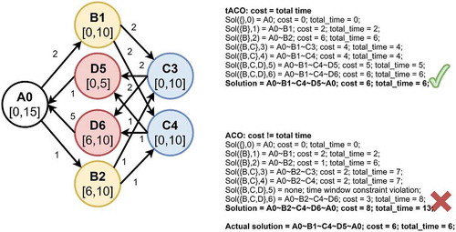
The ExtACO algorithm is not suited for solving the generic cost ACO as in that case the Optimization Invariant does not hold! It is easily conceivable that there could be cases where the overall optimal solution actually contains non-optimal subsolutions as a way of sacrificing a short-term utility gain in order to quickly reach a given time window and thus open up possibilities for later long-term gains. Otherwise we would encounter cases where minimal cost was chosen, but it would have made more sense to choose a more expensive subsolution in order to gain time and thus access to cheaper solutions later on. This kind of strategic long term forward planning is also known as the credit assignment problem (Sutton 1984). Forward constructing dynamic programming would only be possible with much more compute time and memory, because not only the minimum-cost subsolutions would have to be constructed at each stage, but the whole mincost-mintime Pareto front would also be necessary. Of course, the whole problem is avoided if cost equals time – as in tACO – because then the minimum cost subsolution corresponds to the minimum time subsolution and no gains can be made by visiting the same activities and arriving at the same destination – only somewhat later and at a higher cost. An illustration of the problem is given in Figure 1.

Figure 1. Illustration of the steps of the ExtACO algorithm and how it chooses the optimal solution when cost = time vs. how it gets lost when confronted with arbitrary costs (which it is not designed to handle). Letters denote activities and bold numbers denote location id’s. Time window intervals are given between square brackets. Missing arcs may be assumed to have cost and traveling time $\mathrm{\infty }$. Activity durations are integrated into the travel costs and the time windows

GTA*: a greedy time-aware heuristic (*with hints)

Both heuristics presented below work with the same assumptions as ExtACO, i.e. they solve the tACO problem as defined in Section 3.2.

GTA

The heuristic we developed as a baseline – intended to simulate human performance as a proxy for meaningful comparison – is very simple yet surprisingly effective (arguably even super-human). It is defining characteristic is that it requires access to all locations’ time windows and keeps track of the elapsed time as it greedily chooses the closest unprocessed activity location – not based on travel time, but based on estimated time of entry (i.e. travel time plus waiting time). Although it plans only one step in advance, it does so based on complete and precise travel time and opening hours information that is often not readily available to humans when they plan, or if available then not very easy to process en masse.

GTA*

There is a possibility, of course – given its inherently short-sighted strategy – that our greedy time-aware heuristic (GTA) does not find a solution even if there clearly exists (at least) one, as it could choose starting steps in a way that seems prudent at the moment, but makes finishing the tour impossible. It is hard to evaluate the improvement achieved upon a baseline algorithm that cannot solve the problem; therefore, we have modified the GTA algorithm with the following backup plan in case of failure: if regular GTA finds no solution, then run it once more using a fixed, user-given manual ordering of activities. We call this ordering a user ‘hint’, which in practice can either be already encoded in the ordering of records of the problem specification format (e.g. see Table 1) or it could be supplied as an instant feedback through a human-machine interface once the algorithm fails to find a solution unaided. GTA* thus denotes the enhanced version of our GTA algorithm, which employs user hints for activity ordering as a backup plan in case of failure.

Table 1. An example ACO problem instance specification with 5 + 1 activities

Activity	Dur.	DemandStart	DemandClose	FixedLat.	FixedLon.
Start/Goal	0	2019.02.11 6:30	2019.02.11 23:59	47.514895	19.032784
Bakery	5	2019.02.11 6:30	2019.02.11 10:00
Work	480	2019.02.11 6:30	2019.02.11 20:00	47.507163	19.047851
Grocery Store	15	2019.02.11 7:00	2019.02.11 22:00
Cosmetics Shop	20	2019.02.11 8:00	2019.02.11 18:00
Pub	90	2019.02.11 18:00	2019.02.11 23:59

GTA and GTA* both have a linear runtime complexity $O(mn)$ in the number of activities ($m$) and nodes ($n$). Their memory requirement is linear $O(n)$ in the number of nodes and constant $O(1)$ in the number of activities.

Experimental method

We measured the performance of our tACO solvers on real-world data and problems and conducted a statistical analysis of the findings. Although a worst case asymptotic analysis of ExtACO was already performed in Section 4.1, the additional statistical inspection reveals how the theoretical complexity results translate to execution times on a real computer and how the optimal routes compare with those produced by human-like simple heuristics.

Baseline

We define the sequence-hinted greedy time-aware (GTA*) heuristic as our baseline that simulates an extremely well-informed rational human who always makes the best next choice within a one-step-ahead horizon. In contrast with ExtACO, GTA* is still not guaranteed to find a solution if there exists one, but it has at least an increased chance of finding a solution compared to regular, unhinted GTA. We believe it makes sense to employ GTA* as a proxy for unaided human-level performance for two main reasons:

• planning only few steps ahead seems something humans are prone to due to biological limitation, and although one step seems like an over-simplification, it may be roughly counterbalanced by the completeness and precision of information available to the algorithm; and

• the implicit human knowledge of usual opening times of different facilities (e.g. pubs tend to be open in the evening and thus visiting a pub usually becomes a finishing activity for the day) becomes explicitly encoded in the activity sequence hint provided as a backup plan to the algorithm.

It would certainly make sense to conduct a large-scale study trying to pinpoint the most human-like performing algorithm from a given set or family of algorithms in order to establish an even better baseline, but this is beyond the scope of our current discussion. For the already outlined reasons, we treat GTA* as a sufficiently fair and objective baseline somewhat similar to unaided human performance and consider the measured results in terms of cost (i.e. time) reduction an informative estimate.

Real-world data

We downloaded the Budapest road network, public transportation and facilities information data from the online OSM database⁴ (Haklay and Weber 2008). The dataset contained location and opening hours information on 43,998 facilities within the city and the agglomeration. We filtered and cleaned the data with special regard to opening hours, which were stored in a semi-structured way and required us to split some locations into separate logical nodes to account for several time intervals within the same weekday. Thus, we ended up with a dataset of 57,351 locations that offered hundreds of activities. We merged some of the activity clusters based on conceptual likeness (e.g. ‘Café’ and ‘Coffe Shop’). Then, we chose the twenty most popular activities⁵ that also made sense to be considered as spatially flexible demand points (e.g. ‘Office’, ‘School’ and ‘Hospital’ did not make it on the list, as those would be typically spatially fixed activities performed mostly in the same location). For each chosen activity, we sampled 50 locations at random and thus ended up with a 1000-location extract, which formed the basis of all our further measurements. Then, we ran the 1000 nodes through a locally installed OpenTripPlanner⁶ (Hillsman and Barbeau 2011) server and downloaded the symmetric $1000\times 1000$ walking time matrix⁷ over the HTTP REST interface, saving it to disk for later rapid in-memory testing. Although we used walking time for demonstration purposes, our algorithm is independent of this fact and supports any transportation mode, even mixed ones like park & ride. Depending on the up-to-dateness of the data source, travel times might even include semi-dynamic influences like traffic jams and roadblocks. We used walking time for three main reasons, namely: (1) because not all locations were accessible by ‘Car’ or other OpenTripPlanner (OTP) modes like ‘Kiss&Ride’; (2) because of the speed of data access – walking was served most quickly by OTP; and (3) because of the spatial scale of the map and the problems: walking times would enable finer grained analysis of gains achieved in a crammed inner-city environment. We chose the number of exactly 1000 locations for two main reasons: (1) to be able to download the travel time matrix within reasonable time (it took 9–10 hours); and (2) because the smallest cardinality activities among our top-20 list had barely more than 50 entries. Downloading the full $57351\times 57351$ matrix⁸ via the same protocol would have taken $3.75$ years⁹, so we postponed this until we develop an inter-process custom protocol to access OTP functionalities more directly (bypassing TCP and HTTP overheads).

Problem specification format

We chose a minimalistic structured problem instance specification format that together with the extracted map data fully define an ACO problem instance. An example is provided in Table 1. The specification lists the required activities as records in no particular order with the exception of the starting location and activity, which has to be the first record. The activity names can be either one of the activities that already exist in the map or an entirely new kind of activity. In the latter case, fixed demand point coordinates have to be added in the last two columns to have at least one location to plan with. Desired activity duration is specified in minutes, and the activities’ earliest starting time and latest ending time (as preferred by the user who can be entirely unaware of available locations and actual opening hours) are entered in the ‘DemandStart’ and ‘DemandClose’ columns.

45 practical problem instances

We manually created 45 realistic ACO specifications of practical sizes (5–9 activities, 9 specifications for each problem size). All specified problems had one fixed activity (‘Work’), while other activities remained spatially flexible. We ran both algorithms (GTA* and ExtACO) on all of the problems.

Results

Here we present the results of our experiments. The computer running the calculations was an Intel® Core^TM i5-7300HQ CPU @ 2.50GHz$\times$4 64-bit system with 15.5 GiB of RAM. We measured the execution time of computations and the generated tour costs (travel times with and without wait times).

Improved tour quality

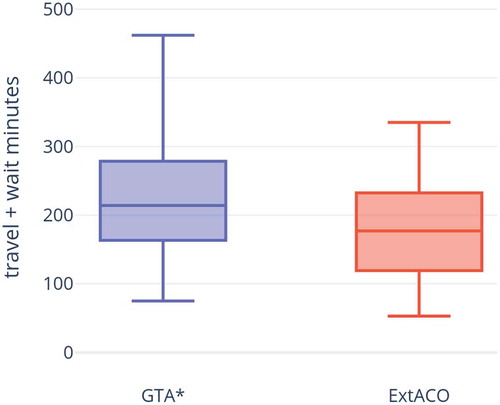
The measurements of the 45 practical problem trials show that GTA* consistently yields very good results that are mostly within $20\mathrm{\%}$ of the optimum. Conversely, the ExtACO exact algorithm delivers an average improvement of $16.65\pm 4.21\mathrm{\%}$ upon our baseline with $90\mathrm{\%}$ confidence. See Figure 2 for reference. Unhinted GTA failed to produce results on 16 out of 45 problems, while hinted GTA failed on 5 out of 45. Since there was no overlap in the failed cases, their sequential application (GTA*) was able to solve all 45 problems; thus, a clear baseline was established. The raw data are given in Appendix Table C1.

Figure 2. Practical 5–9 activity tour costs produced by our Greedy Time-Aware with Sequence-Hinted Backup (GTA*) heuristic and optimum costs produced by our ExtACO exact algorithm for the 45 example problems

Execution time

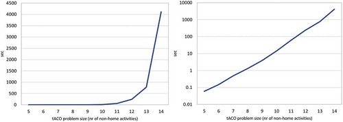
GTA* always runs in 0 seconds while the running time of ExtACO increases with problem size as expected (on average: 0.06, 0.15, 0.49, 1.32 and 3.90 seconds for problem sizes 5–9). ExtACO’s exponential runtime complexity is illustrated in Figure 3: solving a single problem of size 14 took 1 hour and 9 minutes. The detailed solution can be found in Appendix 9. Thus, it is clear that ExtACO can be used in online applications in the regular problem size range of 5–9 activities, while it can be run offline for problem sizes 10–15.

Figure 3. Extaco’s exponential runtime increase on a linear and logarithmic scale

Conclusion

In this paper, we have formally defined the ACO problem and have developed a dynamic programming based exact algorithm that solves the tACO variant of the problem to optimality, albeit with exponential running time $O(2^m{n}^2)$. We have shown that the exponential factor in the asymptotic runtime complexity bound depends only on $m-1$, the number of non-home activities, and since typically $m\ll n$, we claim that the ExtACO algorithm is viable for practical purposes. We are thus able to optimize activity chains of length 5–9 online and length 10–15 offline on maps that have hundreds or thousands of nodes. Our claim is reinforced by our experimental measurements made on 45 realistic problems on a real map of Budapest. The statistical analysis of the data also reveals the practical significance of our work: we achieve $16.65\mathrm{\%}$ average reduction of costs compared to an already quite sophisticated (and arguably super-human) baseline.

We would like to add a few notes on the static nature of our assumptions at this point, relating mainly to activity duration and travel durations but also dynamicity and flexibility in general. Firstly, user preferences like travel modes, activity durations, possible alternative locations and time windows for activities as well as starting and latest finishing times can vary from query to query. Thus, the user can encode their preferred travel mode along with activity location, time and duration preferences as part of the problem instance definition. The user may also apply some of their preferences after being presented with the results of an initial plan and request a more personalized itinerary in a second round of planning. Secondly, incidents like unforeseen store closures, traffic jams and roadblocks that happen only moments before the trip is planned may still find their way into our calculations depending on the up-to-dateness of the data source used. Thirdly, constant recalculation of the trip (which resource-wise is a cheap operation) can give a semblance of quasi-dynamicity as well. A dynamic recommender system could present the user with options regarding the choice of the immediate next target offering $k$ best next locations along with the best performance achievable via each option. Once the choice is made, the system would calculate and present the recommended options for the upcoming choice. This can be done before or even during actual travel, the user making decisions and incorporating their dynamically arising requirements on the fly. Finally, even optimal departure time choice can be performed via a brute-force approach by simply solving for all possible starting times, which is typically only a few hundred problem instances¹⁰.

As for the robustness of our method, it is somewhat implementation-dependent. We have implemented our algorithm such that it will always select the same optimum tour among several equally optimal solutions, so in this regard, we do have some reliability. We also see a practical opportunity in the fact that (mostly due to personal preferences leading to inescapable waiting times) there often are many optimal tours which can be wildly different. As a future development, we can envision advisory services that choose among equi-optimal tours and thus function as a form of unobtrusive marketing.

Future directions for our research will include further exploration of human-like baselines, automatic generation of realistic problems, and a stronger focus on large (more than 15 activities) ACO instances and their applications. We see several main directions for tackling these problem sizes while also remaining practical: either with improvement heuristics (like LKH) or with soft computing metaheuristic methods (genetic algorithms, ant colonies, reinforcement learning), or with linear programming methods that are guaranteed to find the exact solution and that also run fairly well in practice – with the only caveat being the theoretical runtime bound which is even looser than what we present here. An interesting possibility to explore would be to devise a polynomial-time $\epsilon$-approximation method that would give a fairly good starting point for a linear program or a heuristic and could also serve as a quick-fix for the impatient user until a better solution is produced.

We also plan to compare our relatively simple problem formulation that can be solved to optimality with limited resources with more complex and dynamic models. Our goal is to identify those particular circumstances and practical use-cases where our optimally solvable simple model outperforms more realistic ones.

Acknowledgments

The research reported in this paper was supported by the Higher Education Excellence Program of the Ministry of Human Capacities in the frame of Artificial Intelligence research area of Budapest University of Technology and Economics (BME FIKP-MI/SC).

Disclosure statement

No potential conflict of interest was reported by the authors.

Additional information

Funding

This work was supported by the BME FIKP-MI/SC [The research reported in this paper was supported by the Higher Education Excellence Program in the frame of Artificial Intelligence research area of Budapest University of Technology and Economics (BME FIKP-MI/SC).].

Notes

1. Unless $P=NP$.

2. The problem of choosing the best departure time from home (tour starting time).

3. The cutting edge Concorde solver performs the exponential-runtime simplex step an exponential number of times in the worst case (Applegate et al. 2011).

4. Map data and facilities’ opening hours data © OpenStreetMap contributors.

5. [’Restaurant’, ’Hair Salon’, ’Pub’, ’Bakery’, ’Coffee Shop’, ’Bank’, ’Playground’, ’Supermarket’, ’Grocery Store’, ’Fast Food’, ’Cosmetics Shop’, ’Post Office’, ’Smoke Shop’, ’Dessert Shop’, ’Pharmacy’, ’Electronics Store’, ’Park’, ’Gas Station’, ’Gym’, ’ Clothing Store’].

6. http://www.opentripplanner.org/.

7. Size = 2MB.

8. Size = 6.13GB.

9. Estimate arrived at by linear extrapolation: since accessing $\frac{1000\times 999}{2}=499500$ travel times took 10 hours, accessing $\frac{57351\times 57350}{2}=1644539925$ travel times should take $32924$ hours which is 3.75 years. Division by 2 is due to assumption of symmetricity of walking times in both directions.

10. Too early departures are excluded by problem definition, too late departures are excluded by impossibility due to activity durations. Assuming tour starting times are defined with minute precision, there can be at most a couple hundred viable starting times during a typical day, corresponding to a couple hundred problem instances.

Appendix A.

List of notations

Table A1. List of notations

${\mathcal{A}}_k$	activity cluster $k$ (set of all locations that provide activity $k$)
${\mathcal{A}}_z^{(l)}$	set of $l$ activity clusters (possible combinations denoted by index $z$)
$C_{ij}$	cost of travel between locations $i$ and $j$
$C_{ij}(t_i)$	cost function for choosing next location based on ready time at previous
$C(s)$	cost function for a solution sequence (itinerary)
$d$	final location of a subsolution that provides one of the chosen activities
${\delta }_j$	duration of performing activity at location $j$
$\mathcal{E}$	set of directed connections (edges, arcs) between locations
$\mathcal{G}=(\mathcal{V},\mathcal{E})$	directed graph of locations (nodes) and asymmetric connections (edges)
$l$	subsolution length
$m$	number of activities (not counting home)
$n$	number of locations (not counting home)
$N^{(k)}$	largest number of nodes in the union of any $k$ activity clusters
$s=⟨s_0,s_1,\dots ,s_m⟩$	solution sequence (itinerary): a sequence of $1+m$ locations
${\mathcal{S}}_d^{(l)}\left({\mathcal{A}}_z^{(l)}\right)$	$l$ long subsolution with chosen activities ${\mathcal{A}}_z^{(l)}$ and final destination $d$
$t_j$	ready time for departure from location $j$
${\hat{t}}_j$	arrival time at location $j$
${\hat{t}}_{0^{\prime }}$ and $t_{0^{\prime }}$	arrival and ready times when returning to the home vertex
$T_{ij}$	traveling time between locations $i$ and $j$ (${\delta }_j$ included)
$\mathcal{V}$	set of location vertices
$W_j=[w_j^{\prime },w_j^{{ }^{\prime \prime }}]$	time window of location $j$

Appendix B.

Optimal solution to ACO problem size 14

Table B1. ACO problem instance specification with 14 + 1 activities

Activity	Dur.	DemandStart	DemandClose	FixedLat.	FixedLon.
Start/Goal	0	2019.02.11 6:30	2019.02.11 23:59	47.514895	19.032784
Park	15	2019.02.11 6:30	2019.02.11 12:00
Gym	70	2019.02.11 6:30	2019.02.11 23:59
Work	240	2019.02.11 6:30	2019.02.11 16:00	47.507163	19.047851
Bank	30	2019.02.11 7:00	2019.02.11 16:00
Coffee Shop	15	2019.02.11 7:30	2019.02.11 19:00
Smoke Shop	3	2019.02.11 10:00	2019.02.11 23:59
Fast Food	45	2019.02.11 11:00	2019.02.11 14:00
Hair Salon	30	2019.02.11 12:00	2019.02.11 18:00
Post Office	15	2019.02.11 12:00	2019.02.11 20:00
Grocery Store	15	2019.02.11 12:00	2019.02.11 23:59
Playground	45	2019.02.11 16:00	2019.02.11 21:00
Pub	60	2019.02.11 18:00	2019.02.11 23:59
Bakery	10	2019.02.11 18:00	2019.02.11 23:59
Gas Station	10	2019.02.11 20:00	2019.02.11 23:59

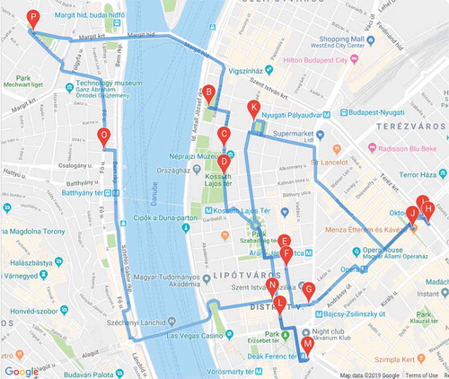
Figure B1. An optimal solution to the 14 + 1 activity problem instance. (P) = Start/Goal

Appendix C.

Experimental results: practical problem sizes (5–9 activities)

Table C1. Experimental results: practical problem sizes of hundreds of locations and 5–9 non-home activities

PID	Acts	Locs	GTA*	ExtACO	impr. %	GTA*-	ExtACO-	impr. %
1	5	179	208	177	14.90	99	119	−20.20
2	6	193	343	319	7.00	128	216	−68.75
3	7	265	255	226	11.37	108	104	3.70
4	8	296	142	77	45.77	137	77	43.80
5	9	328	172	99	42.44	172	99	42.44
6	5	179	199	177	11.06	86	82	4.65
7	6	193	329	315	4.26	151	191	−26.49
8	7	265	246	224	8.94	120	78	35.00
9	8	296	98	53	45.92	90	49	45.56
10	9	328	450	75	83.33	263	75	71.48
11	5	179	195	175	10.26	103	85	17.48
12	6	193	316	306	3.16	184	142	22.83
13	7	265	239	225	5.86	76	63	17.11
14	8	296	75	63	16.00	75	63	16.00
15	9	328	132	99	25.00	132	99	25.00
16	5	179	207	174	15.94	130	77	40.77
17	6	193	327	307	6.12	152	147	3.29
18	7	265	253	224	11.46	155	92	40.65
19	8	296	79	79	0.00	79	79	0.00
20	9	328	169	92	45.56	158	91	42.41
21	5	179	222	187	15.77	148	141	4.73
22	6	193	353	335	5.10	241	222	7.88
23	7	265	266	243	8.65	157	133	15.29
24	8	296	177	124	29.94	177	124	29.94
25	9	328	161	136	15.53	159	136	14.47
26	5	179	204	173	15.20	122	132	−8.20
27	6	193	343	318	7.29	263	206	21.67
28	7	265	248	232	6.45	128	116	9.38
29	8	296	129	129	0.00	128	129	−0.78
30	9	328	462	168	63.64	257	168	34.63
31	5	179	214	181	15.42	141	116	17.73
32	6	193	339	327	3.54	206	180	12.62
33	7	265	259	231	10.81	170	101	40.59
34	8	296	106	83	21.70	101	83	17.82
35	9	328	128	105	17.97	128	105	17.97
36	5	179	218	183	16.06	176	146	17.05
37	6	193	340	328	3.53	255	239	6.27
38	7	265	262	234	10.69	221	137	38.01
39	8	296	125	125	0.00	122	120	1.64
40	9	328	164	144	12.20	164	144	12.20
41	5	179	188	175	6.91	111	124	−11.71
42	6	193	332	307	7.53	254	172	32.28
43	7	265	233	217	6.87	111	100	9.91
44	8	296	113	99	12.39	113	98	13.27
45	9	328	164	128	21.95	164	128	21.95

PID stands for Problem IDs. Acts column contains number of non-home activities ($m-1$). The map contains 50 alternative locations for each activity. Locs column contains number of eligible non-home locations after first removing impossible locations that contradict the user’s activity duration and time window preferences ($n-1$). GTA*- and ExtACO- columns contain total travel times without waiting. ’impr. %’ columns denote improvement percentage compared to baseline GTA*(-).

References

- Abdelghany, A. F., and H. S. Mahmassani. 2003. “Temporal-Spatial Microassignment and Sequencing of Travel Demand with Activity-Trip Chains.” Transportation Research Record 1831 (1831): 89–97. Doi: 10.3141/1831-10.
- Applegate, D. L., R. E. Bixby, V. Chvatal, and W. J. Cook. 2011. The Traveling Salesman Problem: A Computational Study. Princeton University Press. https://press.princeton.edu/titles/8451.html
- Applegate, D. L., R. E. Bixby, V. Chvátal, D. G. William Cook, M. G. Espinoza, and K. Helsgaun. 2009. “Certification of an Optimal TSP Tour through 85,900 Cities.” Operations Research Letters 37 (1): 11–15. doi:10.1016/j.orl.2008.09.006.
- Barach, G., H. Fort, Y. Mehlman, and F. Zypman. 2012. “Information in the Traveling Salesman Problem.” Applied Mathematics 03 (08): 926–930. doi:10.4236/am.2012.38138.
- Cantelmo, G., and F. Viti. 2019. “Incorporating Activity Duration and Scheduling Utility into Equilibrium-based Dynamic Traffic Assignment.” Transportation Research Part B: Methodological 126: 365–390. doi:10.1016/j.trb.2018.08.006.
- Chettibi, T., H. E. Lehtihet, M. Haddad, and S. Hanchi. 2004. “Minimum Cost Trajectory Planning for Industrial Robots.” European Journal of Mechanics A/Solids 23: 703–715. doi:10.1016/j.euromechsol.2004.02.006.
- Christofides, N. 1976. Worst-case Analysis of a New Heuristic for the Travelling Salesman Problem. Technical Report 388. Graduate School of Industrial Administration, Carnegie Mellon University..
- Comi, A., and A. Nuzzolo. 2016. “Individual Utility-based Path Suggestions in Transit Trip Planners.” IET Intelligent Transport Systems 10 (4): 219–226. doi:10.1049/iet-its.2015.0138.
- Cook, W. J. 2012. In Pursuit of the Traveling Salesman. Princeton University Press. https://press.princeton.edu/titles/9531.html
- Dantzig, G., R. Fulkerson, and S. Johnson. 1954. “Solution of a Large-Scale Traveling-Salesman Problem.” Journal of the Operations Research Society of America 2 (4): 393–410. doi:10.1287/opre.2.4.393.
- Dantzig, G. B., A. Orden, and P. Wolfe. 1955. “The Generalized Simplex Method for Minimizing a Linear Form under Linear Inequality Restraints.” Pacific Journal of Mathematics 5 (2): 183–195. doi:10.2140/pjm.
- Esztergár-Kiss, D., Z. Rózsa, and T. Tettamanti. 2017. “Comparative Analysis of Test Cases of the Activity Chain Optimization Method.” Transportation Research Procedia 27: 286–293. doi:10.1016/j.trpro.2017.12.136.
- Esztergár-Kiss, D., Z. Rózsa, and T. Tettamanti. 2018. “Extensions of the Activity Chain Optimization Method.” Journal of Urban Technology 25 (2): 125–142. doi:10.1080/10630732.2017.1407998.
- Fazlollahtabar, H., and M. Saidi-Mehrabad. 2015. “Optimal Path in an Intelligent AGV-based Manufacturing System.” Transportation Letters 7 (4): 219–228. doi:10.1179/1942787514Y.0000000047.
- Grefenstette, J. J. 1985. Proceedings of the First International Conference on Genetic Algorithms and their Applications. Taylor and Francis. https://www.taylorfrancis.com/books/9781315799674
- Gutin, G., and A. Punnen. 2002. Travelling Salesman Problem and Its Variations. Kluwer Academic Publishers. http://site.ebrary.com/lib/wpi/reader.action?docID=10067445
- Hafezi, M. H., L. Liu, and H. Millward. 2018. “Learning Daily Activity Sequences of Population Groups Using Random Forest Theory.” Transportation Research Record 036119811877319. Doi: 10.1177/0361198118773197.
- Haklay, M., and P. Weber. 2008. “OpenStreet Map: User-generated Street Maps.” IEEE Pervasive Computing 7 (4): 12–18. doi:10.1109/MPRV.2008.80.
- Held, M., and R. M. Karp. 1962. “A Dynamic Programming Approach to Sequencing Problems.” Journal of the Society for Industrial and Applied Mathematics 10 (1): 196–210. http://epubs.siam.org/doi/10.1137/0110015
- Helsgaun, K. 2000. “Effective Implementation of the Lin-Kernighan Traveling Salesman Heuristic.” European Journal of Operational Research 126 (1): 106–130. doi:10.1016/S0377-2217(99)00284-2.
- Heydecker, B. G., and J. D. Addison. 2006. “Analysis of Dynamic Traffic Assignment.” In DTA2006 First International Symposium on Dynamic Traffic Assignment.
- Hilgert, T., M. Kagerbauer, T. Schuster, and C. Becker. 2016. “Optimization of Individual Travel Behavior through Customized Mobility Services and Their Effects on Travel Demand and Transportation Systems.” Transportation Research Procedia 19: 58–69. doi:10.1016/j.trpro.2016.12.068.
- Hillsman, E. L., and S. J. Barbeau. 2011. “Enabling Cost-Effective Multimodal Trip Planners through Open Transit Data.” may. https://rosap.ntl.bts.gov/view/dot/20542
- Kona, H., and A. Burde. 2015. “A Review of Traveling Salesman Problem with Time Window Constraint.” IJIRST-International Journal for Innovative Research in Science & Technology 2. www.ijirst.org
- Li, Z.-C., Y. Yin, W. H. K. Lam, and A. Sumalee. 2016. “Simultaneous Optimization of Fuel Surcharges and Transit Service Runs in a Multimodal Transport Network: A Time-dependent Activity-based Approach.” Transportation Letters 8 (1): 35–46. doi:10.1179/1942787515Y.0000000005.
- Li, Z. C., W. H. K. Lam, and S. C. Wong. 2014. “Bottleneck Model Revisited: An Activity-based Perspective.” Transportation Research Part B: Methodological 68: 262–287. doi:10.1016/j.trb.2014.06.013.
- Liao, F., T. Arentze, and H. Timmermans. 2013. “Incorporating Space-time Constraints and Activity-travel Time Profiles in a Multi-state Supernetwork Approach to Individual Activity-travel Scheduling.” Transportation Research Part B: Methodological 55: 41–58. doi:10.1016/j.trb.2013.05.002.
- Menger, K. 1931. “Bericht Über Ein Mathematisches Kolloquium 1929/30.” Monatshefte Für Mathematik Und Physik 38 (1): 17–38. http://link.springer.com/10.1007/BF01700678
- Miller, E. J., and M. J. Roorda. 2003. “Prototype Model of Household Activity-Travel Scheduling.” Transportation Research Record: Journal of the Transportation Research Board 1831 (1): 114–121. doi:10.3141/1831-13.
- Nadizadeh, A., and B. Kafash. 2019. “Fuzzy Capacitated Location-routing Problem with Simultaneous Pickup and Delivery Demands.” Transportation Letters 11 (1): 1–19. doi:10.1080/19427867.2016.1270798.
- Polak, J. W., and B. G. Heydecker. 2006. “The Dynamic Assignment of Tours in Congested Networks with Pricing.” In DTA2006 First International Symposium on Dynamic Traffic Assignment, http://dtasymposium.org/dtasymposia/DTA2006/dta2006_proceedings.pdf
- Rasouli, S., and H. Timmermans. 2014. “Activity-based Models of Travel Demand: Promises, Progress and Prospects.” International Journal of Urban Sciences 18 (1): 31–60. doi:10.1080/12265934.2013.835118.
- Rego, C., D. Gamboa, F. Glover, and C. Osterman. 2011. “Traveling Salesman Problem Heuristics: Leading Methods, Implementations and Latest Advances.” European Journal of Operational Research 211 (3): 427–441. doi:10.1016/j.ejor.2010.09.010.
- Robinson, J. B. 1949. On the Hamiltonian Game (A Traveling-Salesman Problem). Santa Monica: Rand Corp. http://www.rand.org/pubs/research_memoranda/RM303.html
- Sharmeen, F., T. Arentze, and H. Timmermans. 2013. “Incorporating Time Dynamics in Activity Travel Behavior Model.” Transportation Research Record: Journal of the Transportation Research Board 2382 (1): 54–62. doi:10.3141/2382-07.
- Smith, S. L., and F. Imeson. 2017. “GLNS: An Effective Large Neighborhood Search Heuristic for the Generalized Traveling Salesman Problem.” Computers and Operations Research 87: 1–19. doi:10.1016/j.cor.2017.05.010.
- Sutton, R. S. 1984. “Temporal Credit Assignment in RL.” Doctoral Dissertations Available from Proquest https://scholarworks.umass.edu/dissertations/AAI8410337
- Timmermans, H., P. van der Waerden, M. Alves, J. Polak, A. S. Scott Ellis, A. S. Harvey, and K. S. 2003. “Spatial Context and the Complexity of Daily Travel Patterns: An International Comparison.” Journal of Transport Geography 11 (1): 37–46. doi:10.1016/S0966-6923(02)00050-9.
- Timmermans, H., and J. Petrus. 2005. Progress in Activity-based Analysis. Elsevier. https://books.emeraldinsight.com/page/detail/progress-in-activitybased-analysis-by-harry-timmermansProgress-in-Activity-Based-Analysis/?k=9780080445816
- Voigt, B. F. 1831. Der Handlungsreisende, Wie Er Sein Soll Und Was Er Zu Thun Hat, Um Aufträge Zu Erhalten Und Eines Glücklichen Erfolgs in Seinen Geschäften Gewiss Zu Sein. Vol. 7. Schramm. https://books.google.hu/books?id=6zAgAAAACAAJ&dq=Der+Handlungsreisende+wie+er+sein+soll&hl=en&sa=X&ved=0ahUKEwib1qCGhK_gAhVHaVAKHSOACUwQ6AEILjAB
- Xie, C., and S. Waller. 2010. “Estimation and Application of a Bayesian Network Model for Discrete Travel Choice Analysis.” Transportation Letters 2 (2): 125–144. doi:10.3328/TL.2010.02.02.125-144.
- Yao, B., Q. Cao, Z. Wang, P. Hu, M. Zhang, and B. Yu. 2016. “A Two-stage Heuristic Algorithm for the School Bus Routing Problem with Mixed Load Plan.” Transportation Letters 8 (4): 205–219. doi:10.1080/19427867.2015.1110953.