Evaluating the mileage and time efficiency of ridesourcing services: Austin, Texas case

ABSTRACT

Although several studies have attempted to determine the mileage and time inefficiency of ridesourcing services due to concerns about traffic and environmental impacts of these services, all of them provide a point estimate, which does not reflect the uncertainties in the calculation of these estimates. As such this study aims to present the efficiencies as ranges, based on lower and upper limits by identifying drivers' daily activity schedule. Based on an analysis of 200 busiest RideAustin drivers’ trips data (around 282,037 trips over a 6 months period from 1 October 2016) the study finds that the mileage efficiency ranges from 44.3% to 71.6%, while time efficiency ranges from 42.8% to 58.4%. This means that for every 100-miles of a fare-payer passenger, drivers must travel an additional 40 to 126 miles empty. The heterogeneity of the efficiency at the driver level and the efficiency in the temporal dimension were also considered.

KEYWORDS:

• Ridesourcing
• ride-hailing
• transport network companies
• deadheading
• empty miles
• efficiency

Introduction

Ridesourcing services provided by the Transport Network Companies (TNCs, such as Uber and Lyft) have significantly disrupted our travel behavior in the past decade, including mode choice, daily activity, and trip patterns (Conway, Salon, and King 2018). These on-demand ride services enable travelers who request a ride in real-time to connect with potential nearby drivers willing to provide the transportation service via smartphone apps (Shaheen, Cohen, and Zohdy 2016).¹ There is a rapid rise of their popularity worldwide that can be attributed to the many advantages these services offer to the consumers: no need for searching and paying for parking own car, shorter waiting times, real-time tracking of the vehicles, ease of payment, greater availability, and flexibility and often lower costs than traditional taxi services, sometimes even lower than the public transit (Rodier 2018; Schaller 2017; Rayle et al. 2016).

Despite the advantages, there has been some criticism about the environmental sustainability of ridesourcing services, especially in the context of modal share and empty running between dropping off a passenger and picking up the next (Shaheen et al. 2020; Currie 2018). Because of this empty running – also known as deadheading – carbon emissions per passenger mile in a ridesourcing car can be substantially higher than that in a similar privately owned car. Given the rapid increase in ridesourcing, measuring of empty vehicle miles traveled (VMT) is becoming increasingly important in order to understand possible impacts on traffic and associated externalities in cities (Tirachini 2019; Rodier 2018).² The ratio of revenue-miles delivered to total vehicle miles traveled – defined as mileage efficiency here – is also important to understand the fare productivity and wage rate of drivers (Wang and Smart 2020).

There are now some studies investigating the empty running of ridesourcing vehicles based on large trip data (Wenzel et al. 2019; Komanduri et al. 2018; San Francisco County Transportation Authority 2017); however, all of these provide point estimates, which do not adequately reflect the uncertainties in these estimates. Yet, using a point estimate without acknowledging uncertainty can lead to erroneous results if these results are used in other modeling exercises. As such, the first objective of this paper is to address this gap and calculate the efficiencies of ridesourcing services as a range to reveal the uncertainty. This is done by examining the drivers’ daily activity patterns from trip-specific data and by using alternative assumptions about what the drivers do between dropping a passenger and picking up the next one. Also, so far, all the estimates are for one city at an aggregate level and little is known about the possibility that these empty running statistics could vary between days of the week, or between drivers. The second objective of the paper is to understand this potential heterogeneity in the efficiency estimates – both across different drivers, different times of the day and different days of the week. This would enable authorities to properly assess the outcomes of the ridesourcing by considering these uncertainties heterogeneity around empty running. Real trip dataset of RideAustin, a small nonprofit TNC in Austin, Texas has been used to address these research questions.

The rest of the paper is laid out as follows: Literature Reviewprovides an overview of the limited literature on research in this area. Methods and Data section presents a brief description of data and sample and an introduction of the data analysis methods. In Results Analysis and Discussion, the results of the analysis are presented and compared with those in literature. Finally, Conclusions presents some concluding remarks and outlines future work.

Literature review

There is a growing literature on the impact of ridesourcing services on various transportation metrics, e.g. mode choice and travel behavior (Bansal et al. 2019; Liu, Jones, and Adanu 2019; Alemi et al. 2018; Clewlow and Mishra 2017; Hampshire et al. 2017; Rayle et al. 2016); traffic congestion and VMT generation (Beojone and Geroliminis 2020; Tirachini and Gomez-Lobo 2019; Erhardt et al. 2019; Schaller 2017); parking (Wadud 2020a; Henao and Marshall 2019); energy use and greenhouse gas emissions (Wenzel et al. 2019; Rodier 2018); transport employment (Wang and Smart 2020; Xu et al. 2020); and vehicle ownership and equity (Wadud 2020b; Lee, Alemi, and Circella 2019; Ward et al. 2019; Brown 2018). There is an increasing recognition now that the potential benefits of ridesourcing services in terms of environmental and traffic system performance crucially hinges – in addition to the modal shift – on how much of additional ‘empty’ travel is needed to serve a ‘paid’ travel need of a customer (Shaheen et al. 2020; Tirachini 2019; Henao 2017; SFCTA, 2017). Given this importance, several recent studies have attempted to estimate these empty running distances or deadheading distances and corresponding durations.³ Table 1 summarizes the evidence from the literature on the efficiency of ridesourcing services. Ridesourcing efficiency is measured as the proportion of mileage (or time) for which there is a fare-paying passenger in the vehicle to the total distance (or duration) of operation of the vehicle. In other words, it is the ratio of revenue-vehicle-miles (duration) to the total vehicle-miles (duration), and the opposite of deadheading (empty miles/total miles). The reported mileage efficiency estimates run from 55% in Toronto (City of Toronto 2019) to 80% in San Francisco (San Francisco County Transportation Authority 2017). On the other hand, time efficiency varies between 41.3% in Denver (Henao 2017) and 54.3% in San Francisco (Cramer and Krueger 2016).⁴ These differences are primarily due to differences in urban and transport structure, popularity of ridesourcing services, data used and modeling methods and assumptions.

Table 1. A summary of evidence from the literature on the efficiency of ridesourcing services

	Sample description
Research	Driver sample size	Data type	Data period	City/Region	Service provider	Research findings*	Comments
Cramer and Krueger (2016)	Randomlyselected 2,000 UberX drivers	Unknown	December 1 2014 to December 1 2015	Los Angeles New York Seattle	Uber	Mileage efficiency is 55.2% for Seattle and 64.2% for Los Angeles.	The results are directly provided by Uber and potential inclusion of personal travel because if the app is open during those periods.
			From July to October 2015 Average of January 9, April 11, and July 13 in 2015	San Francisco Boston		Time efficiency is 50.3% for Los Angles, 43.6% for Seattle, 51.2% for New York, 54.3% for San Francisco, 46.1% for Boston.
SFCTA,(2017)	Unknown	API Data	Mid-November to Mid-December 2016, excluding dates around the Thanksgiving 2016 holiday.	San Francisco	Uber, Lyft	Mileage efficiency is around 80% for intra-city trips.	Analysis based on approximate vehicle locations at five-second intervals, estimated passenger pick-up times, and active vehicle time on the app. Potential overestimation because empty distances from ride request to pick-up locations were taken as passenger ride.
RockyMountain Institute, (2018) (as cited in Said (2018))	Unknown	Unknown	November 1 2016 to October 31 2017	Chicago New York San Francisco	Lyft	The average distances of cruising, over-heading, and passenger rides are indicated for all three cities.	Given the average distance data of each segment, efficiency in Chicago, New York and San Francisco can be measured as 59.5%, 59.3%, and 67.2%, respectively. Potential inclusion of personal travel in cruising parts.
Henao and Marshall (2019)	1 driver in both services	416 recorded trips data	14 weeks during fall 2016	Denver	Uber, Lyft	Mileage efficiency is 59.2%, while excluding the commuting part it is measured as 70.3%.	Conservative strategy followed to minimize the deadheading (e.g. using two different services at the same time, not taking a passenger whose location is farther than 15 miles, choosing specific start locations, and preferring to work during peak demand times of the day).
Henao (2017)	Same as above					Time efficiency is 41.3%, excluding commuting at the end shift.
George and Zafar (2018)	Unknown	Unknown	October 2017	California	Uber, Lyft	Mileage efficiency is around 60%.	Potential underestimation because most of the drivers use more than one apps at the same time (e.g. trip miles traveled on one platform may be recorded as deadhead miles on another). The results are directly provided by TNC operators.
Komanduri et al. (2018)	Appr. 5,000 drivers	1,494,125 recorded trips data	June 4 2016 to April 13 2017	Austin, Texas	RideAustin	Mileage efficiency is 67%, while time efficiency is 50%, including commuting parts.	Conservative deadhead measurement since the straight-line distances between rides was considered.
Xue et al. (2018)	13,985 drivers	Daily orders data	From the August to December (the year is unknown)	Beijing	DidiChuXing	The average trip distance is about 8.5 km, and the over-heading distance is nearly 25% of the total trip distance.	Given theinformation, overestimated efficiency can be measured as 80% because of excluding cruising part of deadheading.
Wenzel et al. (2019)	Appr. 5,000 drivers	Recorded trips data	October 27 2016 to April 13 2017	Austin, Texas	RideAustin	Mileage efficiency is 55%, including commuting parts, while 64.5% for less than 60 minutes in between consecutive rides.	Applied the correction factor on straight-line distances between locations to represent the street network distance.
Tu et al. (2019)	144,867 drivers	GPStrajectory data	November 24 2015 to November 30 2015	Beijing	Didi ChuXing	The average daily total travel distance of drivers is 129.4 km and the average trip length is 9.7 km, while average daily travel count is 9.	Given the average total travel distance and passenger ride distance, efficiency is estimated at 67.5% – (9x9.7)/129.4.
City of Toronto (2019)	Unknown	Unknown	For March 2017 and September 2018	Toronto	Uber	55% of the total VMT was spent in-service.	The results are directly provided by Uber and details of findings are not known.

it should be noted that some studies may include the pooled ridesourcing trip (e.g., UberPool and LyftLine) (Henao 2017; Henao and Marshall 2019). Clearly mentions inclusion of pooled trips, others do not explicitly mention anything about pooling.

It is important to note that even the same data led to different findings due to differences in modeling methods and underlying assumptions. For example, both Komanduri et al. (2018) and Wenzel et al. (2019) used RideAustin data but report efficiencies of 63% and 55%, respectively. This is because (1) Komanduri et al. (2018) assumed that the driver is off duty (i.e. taking a break) if the gap between two passenger trips is more than 30 minutes, while the cutoff point is 60 minutes in Wenzel et al. (2019); (2) Komanduri et al. (2018) assumed a 2 mile and 5-minute commute trips to the first and last trip of each shift, while Wenzel et al. (2019) attempt to identify driver’s residential location using the first trip locations; (3) Komanduri et al. (2018) assumed straight-line distances for empty trip lengths, while Wenzel et al. (2019) used a correction factor of 1.4 to straight-line distances. This clearly shows that the results can vary by as much as 15% even using the same data as a result of different modeling assumptions.

Each of the studies in Table 1 reports only a point estimate for the efficiencies, not recognizing the uncertainties associated with the assumptions in such estimates as revealed above. There are also no obvious ways of identifying which assumptions or estimates are closer to the reality, without further data. These studies are also focused on providing one average estimate overall and do not investigate the heterogeneity of ridesourcing efficiency between different drivers or different times. As such in this paper we focus on (a) measuring efficiency of ridesourcing as a range: the upper limit represents the best-case efficiency that is based on minimum traveling between a passenger drop-off and next pick-up, while the lower limit represents the worst-case efficiency that is calculated from a potential maximum traveling between rides (cruising); (b) identifying and calculating any heterogeneity of the efficiency estimates at a driver level; (c) investigating how the efficiency changes according to the day of the week and a certain period of the day. Like Komanduri et al. (2018) and Wenzel et al. (2019), RideAustin dataset was used in this study and similar strategy was followed to identify empty trips. But, in measuring empty trips, rather than using straight distance or a correction factor, the real street distance is considered by getting direction between locations via Google Distance Matrix API.

Methods and Data

Data source and sample description

Although some large taxi (e.g. yellow and green taxi trip records in NYC⁵) and ridesourcing (e.g. City of Chicago⁶) trip datasets are publicly available for some U.S. cities, only a few datasets are suitable to analyze the efficiency of service by considering empty trips of drivers. RideAustin trip record is one such dataset as it allows identifying a driver’s daily trip patterns by following a driver identifier (ID). RideAustin, a nonprofit TNC, entered the ridesourcing market in Austin, Texas in 2016, shortly after the two market leaders Uber and Lyft shut down their operations due to disagreements over local regulations (Hampshire et al. 2017). Their dataset consists of a total of 1,494,125 rides that are conducted by approximately 5,000 drivers for a period of 11 months from June 4 2016 to April 13 2017 (Ride Austin 2017). The data provides individual trip level information, including the location of trip origins and destinations (around 100 m accuracy to protect privacy), recorded trip length, corresponding fare, and the timestamp at following five points along each ride: when the ride request was dispatched to a driver; when the driver accepted the dispatched request; when the driver reached the passenger pick-up location; when the ride started; and when the ride was completed (Wenzel et al. 2019).

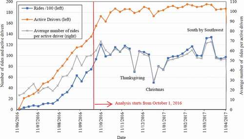
The analysis in this study focuses on data from 200 drivers who have the highest trip numbers in the dataset. The resulting cleaned dataset has data from 200 drivers covering 328,725 trips. Although this is only 4% of the drivers in the dataset, they serve around 20% of all trips. Figure 1 shows the weekly distribution of their total number of rides, active drivers each week, and the average number of rides per drivers. As can be seen in the figure, with the increasing number of active drivers in the system the total number of weekly rides increased significantly in the first 4 months and then stabilized around 10,250 weekly rides. The lowest ridership was during Christmas and the highest during a music festival South by Southwest. Our analysis focuses on the last 6 months of relatively stable period, starting from October 1 2016, covering 282,037 trips. Drivers completed an average of 1,410 trips during that whole period, ranging from 640 to 3,132 trips. The number of working days for drivers varied between 53 and 191 days, while the average number of worked was 140 days. Drivers completed on average 10 trips per working day, the busiest one carried out nearly 20 trips, while the lowest one served almost 5 trips.⁷

Figure 1. The total number of rides, active drivers, and the average number of rides per driver, by week of selected 200 drivers.

Analysis methods

Ridesourcing drivers travel patterns

The term deadheading refers to the distance traveled without passengers or freight and it is often used for the taxi and trucking industry. Exclusive to ridesourcing services, Henao and Marshall (2019) suggested four specific segments of deadheading: commuting from driver residence; cruising for a ride; from dispatch to the pick-up location (over-heading); and commuting at the end of shift. Although commuting is important for VMT and energy use calculations, the driver residences are not revealed due to privacy reasons. We also believe commuting is part of any other job (these drivers may have had to commute to their work had they not been driving for TNCs). As such we focus on driver travel pattern in-between time when the first ride was started and when the last ride was completed for each shift.

Based on the RideAustin dataset, there are two major uncertainties regarding the time between the trips: (a) whether the driver is actively seeking a ride, and (b) what is the driver doing when he/she is actively seeking a ride but does not have a passenger. For (a), we assume that the driver is active as long as the time gap is below 60 minutes (but we test the sensitivity using other durations); otherwise, he/she is taking a break or commuting. For (b) we use two opposing scenarios of Kontou et al. (2019): the driver is driving continuously in search of a passenger for the worst-case, and the driver waits for the next ride request in the last drop-off location for the best-case. While the reality is surely somewhere in between, without any evidence of what actually happens, we prefer to use these two extremes as the bounds of empty miles. Note that for our empty duration calculations, this problem is less important.

Sample of time flow of RideAustin drivers and travel segments between two rides and corresponding information on locations and time are shown in Figure 2. Two different situations are possible for deadheading according to time when the ride request was dispatched to the driver. The first one represents a new passenger ride request was dispatched to the drivers after the previous ride ends (Figure 2b). In this case, drivers follow these patterns, respectively: cruising for a new ride or wait for the new ride request while parking; ride request is dispatched to a driver; ride request is accepted by a driver; traveling to a passenger pick-up location. If a driver does not park after the end of a completed ride and he/she cruises around until the receipt of dispatching another request, this situation represents the maximum traveling case of a driver and the corresponding distance traveled between this period represents the maximum empty trips distance. On the other hand, the second case represents the new ride request is dispatched to drivers before the previous passenger ride ends (Figure 2b). In this situation, drivers know where to travel after the current ride ends. This eliminates the cruising for a ride segment of deadheading and represents the minimum traveling case. The time between previous passenger ride ends and reached on the passenger pick-up location represents to empty trip duration, while the distance between these two locations represents to conservative empty trip distance. This is also equivalent to parking and waiting until drivers get the next trip is dispatched for the first scenario (Figure 2c).

Figure 2. (a) Sample of RideAustin drivers’ working time flow, with empty trip segments shown in the dashed line. Travel segments of drivers in between two rides: (b) dispatched time after previous ride end; (c) dispatched time before previous ride end.

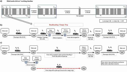
As it was earlier mentioned, RideAustin data includes the timestamp at five points along each ride. This provides an opportunity to calculate durations of all segments in the driver's travel pattern to be analyzed. Figure 2 shows the analysis of driving travel segments and corresponding duration and distance terms of ridesourcing components, which are explained in the below:

• t₁ = time from the previous ride was completed to when the next ride request was dispatched to a driver (Waiting or cruising for a ride).

• t₂ = time from ride request was dispatched to a driver to driver accepted the dispatched request (Driver response).

• t₃ = travel time from ride request location to passenger pick-up location (Over-heading).

• t₄ = waiting time for the ride start at pick-up location (Waiting for ride start).

• t₅ = travel time from the passenger pick-up location to drop-off location (Passenger ride duration).

• t₆ = estimated travel time from previous ride end location to next ride start location (conservative empty trip duration considering traffic condition based on Google Maps). This term is taken as t₃ if dispatched time before previous ride end (Figure 2c).

• d₁ = travel distance from the passenger pick-up location to drop-off location (Passenger ride distance).

• d₂ = distance from previous ride end location to next ride start location (Conservative empty trip distance based on Google Maps).

Given time and distance terms above, parameters, which are used in the calculation of ridesourcing efficiency, are calculated by following equations for each driver for each shift i and ride j:

(1) $Emptyduration=\sum _{i=1}^n\left(\sum _{j=2}^m{t}_{1\left(i,j\right)}+t_{2\left(i,j\right)}+t_{3\left(i,j\right)}+t_{4\left(i,j\right)}\right)$(1)

where m is the last ride of each shift i and n is the last shift;

(2) $Vehiclehourstravelledwithpassenger\left(PHT\right)=\sum _{i=1}^n\sum _{j=1}^m{t}_{5\left(i,j\right)}$(2)

(3) $Vehiclemilestravelledwithpassenger\left(PMT\right)=\sum _{i=1}^n\sum _{j=1}^m{d}_{1\left(i,j\right)}$(3)

(4) $Conservativeunoccupiedvehiclehourstravelled\left(cUVHT\right)=\sum _{i=1}^n\sum _{j=2}^m{t}_{6\left(i,j\right)}$(4)

(5) $Conservativeunoccupiedvehiclemilestravelled\left(cUVMT\right)=\sum _{i=1}^n\sum _{j=2}^m{d}_{2\left(i,j\right)}$(5)

The waiting time for the ride start at the pick-up locations (t₄) was taken as zero for the measurement of the maximum traveling scenario of a driver during an empty period (Eq. 1)(1) $Emptyduration=\sum _{i=1}^n\left(\sum _{j=2}^m{t}_{1\left(i,j\right)}+t_{2\left(i,j\right)}+t_{3\left(i,j\right)}+t_{4\left(i,j\right)}\right)$(1) . Apart from that, since analysis focuses on the period from the first ride starts time to last ride ends of each shift, ‘j’ starts from the second trip of each shift for the empty trip parts.

Ridesourcing efficiencies

The mileage efficiency range is determined by comparing the vehicle miles traveled with a passenger (PMT) versus total VMT for both minimum and maximum cruising scenarios. The lower limit of the range is calculated using Eq. (6(6) $Mileageefficiency\left(Lowerlimit\right)=\frac{PMT}{PMT+eUVMT}$(6) ).

(6) $Mileageefficiency\left(Lowerlimit\right)=\frac{PMT}{PMT+eUVMT}$(6)

where:

(7) $eUVMT=\frac{PMT}{PHT}\left(Averagetripspeed\right)\times Emptytripduration$(7)

Empty trip duration in Eq. (7(7) $eUVMT=\frac{PMT}{PHT}\left(Averagetripspeed\right)\times Emptytripduration$(7) ) represents the time from the previous ride ends to driver reached on the next passenger’s pick-up location (t₁ + t₂ + t₃).

While for the upper limit of bound:

(8) $Mileageefficiency\left(Upperlimit\right)=\frac{PMT}{PMT+cUVMT}$(8)

The time efficiency is defined here as the ratio of vehicle hours traveled with passengers (PHT) to total vehicle hours, and it is calculated by using the following equation:

(9) $Timeefficiency=\frac{PHT}{PHT+Emptyduration}$(9)

In calculating the efficiency of drivers, if passenger ride is completed in-between two empty duration that is exceeding the chosen time limit, passenger ride distance and duration were not included in the analysis (Figure 2a). Moreover, the additional VMT term is not considered if the new ride request is dispatched to drivers before the previous passenger ride ends (Figure 2c). In the calculation of eUVMT, the average trip speeds of drivers were used. However, in practice, drivers can drive more slowly during the empty-running period, or may not drive during the whole duration. Thus, the calculated maximum VMT is likely overestimated here, but this represents the theoretical worst-case scenario, which is the objective here.

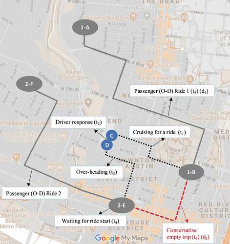
Components of a sample of two consecutive rides are displayed in Figure 3, which illustrates how conservative empty trip miles are estimated in this study. As mentioned earlier, the locations of the drivers in the dataset are not known when: (1) the ride request was dispatched to the driver (C) and (2) when the dispatched request was accepted (D) by the driver. For these reasons, conservative empty trip distances between rides were measured by getting directions from previous ride`s passenger drop-off locations (1-B) to next ride’s passenger pick-up locations (2-E) through Google Maps. This is indicated by the red dashed line in the figure and analyses of 200 drivers were performed by using Google Distance Matrix API considering historical traffic conditions according to departure time; therefore, empty trip lengths reflect the street network distance. The distances between two locations and estimated corresponding duration of traveling by vehicle were obtained at the end of this step. This represents the strategy that drivers park just after completing each ride and wait for the next request, instead of cruising around to reduce the empty trip distance. On the other hand, while calculating the maximum empty trip distance, it is assumed that drivers travel during the whole idle period without parking, which is indicated by the black dotted line (Figure 3).

Figure 3. Components of two consecutive trips sample (representational, does not reflect the actual ride performed)

Results Analysis and Discussion

Travel details of drivers based on fare-paid trips

Based on the data of the busiest 200 drivers in RideAustin, about 44% of total 282,037 passenger trips completed less than 3 miles long, while approximately 14% were longer than 10 miles. The average passenger trip length was 5.1 miles, while at an individual driver level it varies from 3.8 to 8.6 miles. Considering duration, around 71% of passenger trips were completed within 15 minutes, with a third completed between 5 and 10 minutes. The average paid trip duration was about 13 minutes. These results are broadly consistent with the findings of Schaller (2018), who reported that trip length is typically 6.1 miles in U.S. cities although trips in large, densely populated metro areas tend to be shorter (4.9 miles).

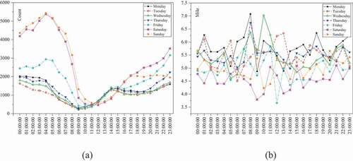
Majority of fare-paid trips were started at nights (8–12 p.m.) and late-nights and early-mornings (12 p.m–6 a.m.), compared to mornings (see Figure 4a). More than half of the passenger rides (60%) are completed between Friday and Sunday. This suggests that RideAustin users likely generally use this service for leisure or discretionary trips. While considering the average trip length, weekday trips are longer than weekend trips. Moreover, considering the time of day, generally morning peak trips in weekdays are longer than weekend trips (Figure 4b).

Figure 4. (a) The number of trips by the time of the day. (b) Average miles per trip by the time of day

Ridesourcing efficiency rate

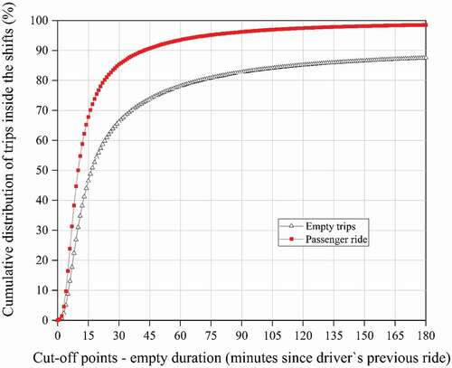
Figure 5 displays the cumulative distribution of passenger ride and empty trips that included in the analysis in drivers’ shift based on the cutoff points. In the figure, the black line with triangles represent the distribution of empty trips that were not undertaken during a break (or during commute), while the red line with square markers shows the cumulative distribution of passenger trips that were included in the shift (see Figure 2a). Black triangular dots also display the number of passenger trips that started within a defined period (on x-axis) after the last trip. More than half of all fare-paid rides (56%) were started within 20 minutes of the end of the previous passenger ride of the drivers, while approximately another 20% of rides were started between 20 and 45 minutes after the end of a driver’s previous ride. As mentioned earlier (in Section 3.2.1), we assume the cutoff point for active ride seeking by the drivers was 60 minutes, indicating nearly 78% of the started trips fall within this range. This means that approximately 22% of empty trips are outside the analysis for 60 minutes cutoff time limit and these trips are considered to be taking place at the start of the day or after the day or break periods (see Figure 2a). Given the number of passenger trips included in the shifts of each driver – the example is shown in Figure 2a – approximately 93% of the total passenger trips are included in the analysis. This indicates that about 7% of the total passenger ride is completed between two idle times that are longer than 60 minutes.

Figure 5. Cumulative distribution of passenger rides and empty trips in the drivers’ shift according to cutoff time limits (for 200 busiest drivers)

Mileage efficiency rate

Based on the analysis of 60 minutes limit in-between rides, the mileage efficiency ranges between 50.0% and 66.5%. This means that for every 100 miles of VMT, between 50 and 66.5 miles is fare-paid vehicle miles, or – borrowing from air transport management – revenue vehicle miles. This represents a 33% difference between the high and low efficiency estimates, which arises from the differing assumptions about what the drivers do in between two passenger rides.

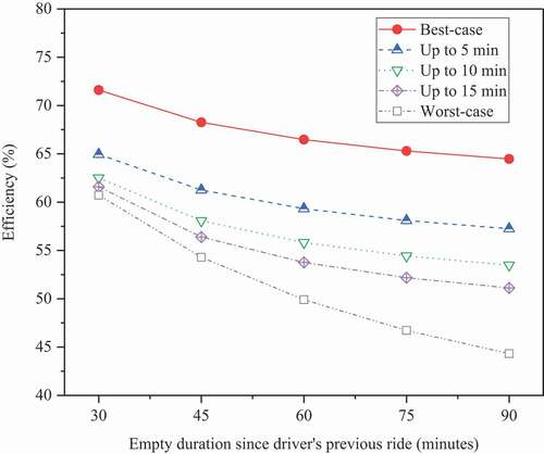
According to Wenzel et al. (2019), any travel started more than 60 minutes after the previous ride end includes at least some personal travel such as dropping off a child from school. On the other hand, Nair et al. (2020) emphasized that ridesourcing drivers could wait for the new request for more than an hour, based on anecdotal evidence from drivers’ forum. Due to this uncertainty, five different cutoff periods were investigated to understand how the efficiency estimates changes depending on the chosen break/commute cutoff periods. We also test three different scenarios for calculating empty VMT. Instead of cruising around during the whole idle time for our lower efficiency estimate, it is assumed that drivers continue to seek a new ride up to the first 5, 10, or 15 minutes and then park. Since drivers must travel between two passenger rides under these scenarios, the maximum empty trip distance was determined by the summation of conservative empty trip distance (Eq. (5)(5) $Conservativeunoccupiedvehiclemilestravelled\left(cUVMT\right)=\sum _{i=1}^n\sum _{j=2}^m{d}_{2\left(i,j\right)}$(5) ) and additional VMT. Here, additional VMTs were estimated by multiplying the average speed of drivers with additional times, which is time differences between empty duration and duration given by GoogleMaps. The results of these sensitivity tests are illustrated in Figure 6. As can be expected, higher efficiencies are calculated for lower cutoff limits of empty trips, and it is observed that the efficiency range is widening as we increase the cutoff limit. For the lower empty duration limits, cruising time is also short, and the estimated efficiencies (e.g. up to 15 minutes cruising) are relatively close to the worst-case line.⁸ However, cruising time have a significant impact on ridesourcing efficiency. For example, the estimated efficiencies of best-case scenario (immediate parking with no cruising) drop off remarkably even for 5 minutes of cruise time, which is a very realistic scenario. These findings may provide insight into the recent debate on the restriction of drivers ‘cruising time’ for new passengers (Hawkins 2019). Due to unknown cutoff time for break periods, the main inference from the figure is that the mileage efficiencies can vary between 44.3% and 71.6% that covers all assumptions, although both the extreme ends are highly unlikely. This equates that for every 100-miles with a fare-payer passenger, drivers must travel an additional in-between 40 and 126-miles. Here, additional empty miles boundaries – cUVMT and eUVMT – were estimated by using Eq6(6) $Mileageefficiency\left(Lowerlimit\right)=\frac{PMT}{PMT+eUVMT}$(6) and Eq8(8) $Mileageefficiency\left(Upperlimit\right)=\frac{PMT}{PMT+cUVMT}$(8) , where PMT was taken 100 miles. Given it is highly unlikely that the drivers continuously cruise or always park immediately after a trip, it is more likely that the mileage efficiency lies between 52% (75-minute cutoff, up to 15 min cruise) and 62% (45-minute cutoff, up to 5 min cruise) – this is still a difference of around 20%.

Figure 6. Mileage efficiency by time cutoff points for breaks

Our findings are broadly consistent with the efficiency estimates in previous studies (excluding the commuting segments of deadheading for a like-for-like comparison) stated in Table 1. Clearly, the mileage efficiencies of the two studies that use RideAustin data – Wenzel et al. (2019) and Komanduri et al. (2018) – fall within our range. Barring San Francisco, all mileage efficiency estimates in the literature fall within our range, despite differences in city characteristics. San Francisco efficiencies were clearly overestimated because their occupied miles actually included the empty miles from ride request to passenger pick-up locations. This suggests that the estimated range can be taken into account when evaluating the possible deadheading related effects of these mobility services. However, the findings of some cities may be underestimated because most of the drivers use more than one apps at the same time (Henao 2017). For instance, trip miles traveled on one ridesourcing platform may be recorded as deadhead miles on another. Apart from that, results may include personal travel such as running personal errands because if the app is open, miles driven by drivers during those periods were recorded as deadheading VMT (George and Zafar 2018). However, since the findings of RideAustin are based on the data collected when two sector giants (Lyft and Uber) in the USA were temporarily out of service in the city, the results are possibly more applicable for cities where drivers are permitted to use only one platform.

Driver heterogeneity of mileage efficiency

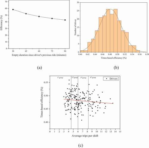
Even though the analysis in this study focuses on data from 200 busiest drivers, there can still be heterogeneity between drivers due to different working patterns. Figure 7 shows the distribution of the mileage efficiency of these 200 drivers for the 60 minutes limit between trips. Considering individual driver level, efficiency for best-case scenario varies from 59% to 77%, while for worst-case, which is continuous cruising without parking, differs between 45% and 59% (Figure 7a). However, it should be noted that the mileage efficiency of most drivers varies from 65% to 70% in the best-case, and 47% to 52% in the worst-case. In order to assess heterogeneity further, the effect of average shift duration and the average number of trips per shift on efficiency was also taken into account. Figure 7b displays the distribution of drivers according to their average shift duration, including the best fit lines. The figure shows that even though drivers consume almost the same amount of time per shift on average, there are significant differences in their efficiency. For example, across the drivers with an average of 150 minutes per shift, that there is nearly 10% difference in their best-case efficiency. Considering the average rides per shift a similar tendency is observed between drivers (Figure 7c). This heterogeneity is likely caused by drivers following different working strategies (e.g. preferring locations where there is a high probability of receiving a new ride request or time when rider demand is high). Using the best-case scenario, we observe a pattern of lower efficiencies for drivers who work longer and serve more trips. This is likely to be expected, as these drivers possibly work through periods of off-peak demand that result in longer gaps between journeys. On the other hand, drivers working for shorter periods likely to optimize when they drive and provide more service during peak periods. However, the uncertainties (differences between best and worst case) appear to reduce as number of trips per shifts increase (Figure 7d). Table 2 presents the average efficiencies for four quartiles of driver groups (50 drivers per group) based on trips per shift. It can be seen that the lower efficiency trend in best-case for drivers who make more trips per shift. On the other hand, no significant trend is observed in the worst-case scenario, which is almost the same for every driver group. It is difficult to compare their worst-case efficiency as there is high uncertainty about what drivers do in their empty time.

Figure 7. Distribution of the mileage efficiency of drivers for 60 minutes time limit: (a) by density; (b) by average working time per shift; (c) by the average number of trips per shift; (d) by the differences between scenarios

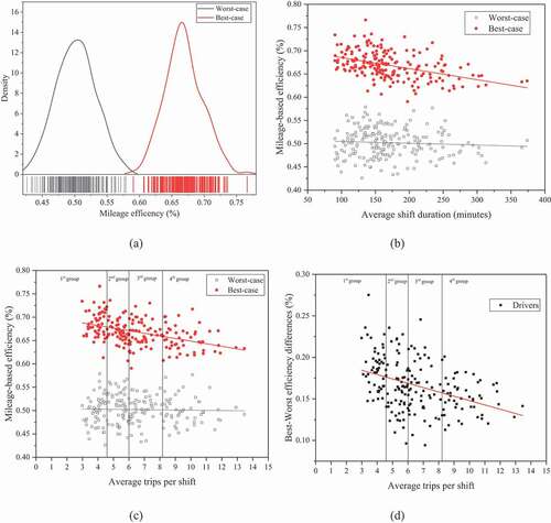
Table 2. Mileage efficiency rate statistic according to the category of drivers

Driver category	Trips per shift (n)	Average trips per shift	Worst-case mileage efficiency (%)				Best-case mileage efficiency (%)
			Min.	Max.	Mean	S.D.	Min.	Max.	Mean	S.D.
1^st group	n ≤ 4.6	4.0	42.62	57.90	50.02	3.21	61.33	76.63	68.70	2.84
2^nd group	4.6 ≤ n < 6	5.4	44.21	56.73	50.83	3.26	60.66	73.60	67.10	2.26
3^rd group	6 ≤ n < 8.2	6.8	43.30	54.83	50.06	2.80	59.05	73.01	66.45	2.78
4^th group	8.2 ≤ n	9.7	44.65	57.69	49.92	2.94	60.74	71.72	65.11	2.59

The average trip distances traveled per shift can be used to determine the total travel distance for drivers per shift, excluding commuting and personal trips during a break period. For example, drivers in group 4 (those with the highest trips per shift can give us more critical information about the battery range) traveled around 44 miles, where the minimum is 33 miles, and the maximum is 66 miles. Based on these efficiency findings, the average conservative total VMT of drivers per shift can be measured as about 68 miles (average PMT/mean best-case efficiency), while the maximum VMT of drivers is estimated around 88 miles (average PMT/mean worst-case efficiency). This can be important to evaluate the electrification of ridesourcing vehicles such as determining optimum battery range that will not affect drivers daily working progress.

Temporal heterogeneity of mileage efficiency

In addition to driver heterogeneity, understanding temporal differences in mileage efficiencies is also important in evaluating the impact of ridesourcing services on transport externalities. Figure 8 displays how the mileage efficiency changes according to the day of week and time of day. Although the efficiencies in the best-case scenario did not show a remarkable difference between days (except Monday and Tuesday), the highest efficiency is observed on Saturday (Figure 8a). However, their corresponding worst-case efficiency shows an increasing trend toward the end of the week (Figure 8b). In other words, the uncertainties (differences between best and worst case) appears to decrease through the weekends. This indicates that drivers worked more effectively on weekends compared to a weekday. On the other hand, the lowest efficiency is observed on Tuesday. This may be because drivers complete fewer trips on Tuesdays compared to other days of the week, as seen in Figure 4a. Also, the average trip miles on Tuesdays and Mondays are relatively higher than others, which may result in longer idle trips for the driver (see Figure 4b).

Figure 8. Mileage efficiency: by day of the week (a) worst-case, (b) best-case scenario; (c) by the time of day. (d) Number of drivers worked according to day of week and time of day

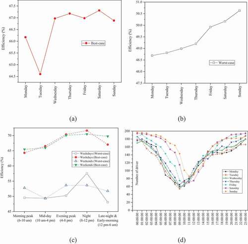
Considering the time of the day, high efficiency can be observed for night trips for all days of the week. For the weekdays, trips completed at night have higher efficiency compared to mid-day and evening peak for both scenarios, also late-night and early-morning trips are more efficient than morning peaks based on the conservative case (Figure 8c). Figure 8d shows the number of working drivers in days and hours during the analyzed period. In other words, the graph shows how many drivers were working among 200 drivers in a given day and time period. It is clear that more than half of the drivers did not work during morning rush hours. On the other hand, most of the drivers worked during early and late nights. Also, Fridays and weekends were the most popular working days for drivers.

Time efficiency rate

Unlike mileage efficiency, there is less uncertainty in time efficiencies, since no assumption is needed as to whether the vehicles are moving or parked in between fare-paying trips. Assuming a 60 minutes cutoff in-between two rides, ridesourcing efficiency in terms of times was estimated at about 48.0%. In other words, the deadhead times were measured as nearly 52.0%. This indicates that drivers spend more time without passengers than with one in the vehicle. However, there is no observation in the ridesourcing industry that provides a more accurate indication about the upper time limit of drivers that are able to wait for the new request. Therefore, it is measured that the efficiency is ranging between 42.8% and 58.4% based on different cutoff time limits (Figure 9a). This estimated range on time efficiency of ridesourcing due to uncertainties on drivers break time are broadly consistent with the previous studies that are stated in Table 1. Although many factors such as city and user characteristics, time of data acquisition and method of analysis are different, almost all time-based efficiency estimates in the literature fall within our range. This is not surprising, given the objective of this paper is to estimate the range to understand the uncertainty these estimates.

Figure 9. Time efficiency rate (a) by the time cutoff points for break (b) distribution of 200 drivers for 60 minutes time limit (c) by the average number of trips per shift

Driver heterogeneity of time efficiency

Time efficiency is especially important to understand driver earnings. Given the heterogeneity between the drivers, a difference of approximately 15% was measured between the efficiency of the drivers, and this difference ranged from 41% to 55% (Figure 9b). However, the time efficiencies of most drivers vary from 43% to 53%. The low-efficiency results are likely due to drivers working during off-peak periods that face low driving demand and results in a long wait between journeys. On the other hand, high efficiency can be observed in drivers who take more breaks or who do not work regularly. Approximately 75% of 200 drives have less than 50% efficiency. As the average number of trips per shift increases, the average time-based efficiency of the drivers reduces (Figure 9c). It would be useful to investigate if less-frequent drivers have a better time-efficiency given they would likely work only during the high-demand periods resulting in smaller wait times; however, that is beyond the scope of this work.

Temporal heterogeneity of time efficiency

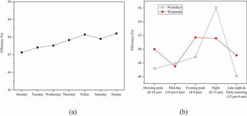
Considering the day of the week and time of the day, a similar trend was observed to mileage efficiency. The highest efficiency is estimated for Saturday trips (Figure 10a). Over weekdays, the highest efficiency is observed at nights compared to other time periods (Figure 10b). Moreover, Figure 10 shows that weekends trips are generally higher efficiency than a weekday. As it is expected, the results show that time efficiency has similar trends to worst-case mileage efficiency. This is because the worst-case scenario was calculated based on the empty durations, so it is highly related to time efficiency.

Figure 10. Time efficiency (a) by day of the week (b) by the time of day

Conclusions

This paper has made three contributions to our understanding of the efficiency of ridesourcing services. Firstly, we calculate the efficiency using actual road-network-based distances (unlike previous use of straight-line distances or correction factors). Secondly, we highlight the importance of assumptions in estimating the efficiencies and provide a range of estimates instead of point estimates as in previous literature in order to properly reflect the uncertainties. Thirdly, we estimate the heterogeneity in these efficiency estimates – both for different drivers and different times of the day and days of the week. Based on the analysis of RideAustin data, we estimate that the mileage efficiencies – excluding commuting – can vary between 44% and 71% depending on the underlying assumptions about cutoff time for breaks and end of shifts, and on whether the vehicle is parked between the trips or not. Our best estimate is narrower – between 52% and 62% – which still represents a difference of around 20%. This highlights the significance of assumptions in deriving these estimates and suggests caution while using single point estimates. Considering the time-efficiency, the estimates are narrower between 45% and 52%. Further research on drivers’ behavior in between the passenger rides will help narrow these ranges.

There is substantial heterogeneity in the efficiency estimates – particularly with respect to drivers, times of the day and days of the week. The highest efficiency was observed during weekends, which possibly reflects the higher volume of patronage during these days. Night trips had higher efficiencies compared to other times of the day, again reflecting the higher volume of trips during these times. These findings are consistent with previous studies showing that Uber and Lyft services are mostly preferred by users on weekends and night times (San Francisco County Transportation Authority 2017; City of Toronto 2019). Between drivers, those who work longer hours and more trips per shift on average tend to have lower efficiencies, although there is a wide variation between driving similar number of trips per shift. Given our results are based on around 20% of all RideAustin trips, further analysis of the full dataset may allow a deeper understanding of the heterogeneity.

Our results confirm previous findings that ridesourcing services generate substantial additional VMT in between two paid rides. Even in the best-case scenario where the driver immediately parks after a passenger drop-off, they still travel empty half of the miles for carrying passengers. Considering the whole activity scheme of the drivers, including commuting (e.g. Wenzel et al. 2019) a considerable amount of deadheading mileages is added to the urban transportation system. Therefore, at an individual trip level, even if the ridesourcing trip replaces an existing vehicle-mile, the implications for the system are substantially larger. As such there are reasons to remain concerned about their effects on congestion and associated vehicle emissions in the urban transportation network, especially for cities that have already congested streets.

Our results highlight the uncertainties associated with existing estimates of deadheading of ridesourcing services, with implications for increases in VMT, congestion or carbon emissions; however, the net effects on VMT or carbon emissions require further knowledge about the travel behavior of users (e.g. modal substitution effects) and passenger occupancy in the ridesourcing trips. Some of these have been addressed in a separate strand of literature (e.g. Clewlow and Mishra 2017; Henao 2017 for modal shift; Mohamed, Rye, and Fonzone 2020 for occupancy, etc.) and suggest the modal shift implications can also be adverse from an environmental and congestion perspective.

To reduce the empty miles of ridesourcing services, the implementation of effective curb space management is as important as increasing the occupancy level of these services (Shaheen et al. 2020). For example, designated short-time vehicle parking/waiting locations in dense areas, particularly in downtown recreational and sometimes employment areas, could help reduce the cruising of ridesourcing vehicles around cities with empty seats. Additionally, given the substantial wait between passenger trips, construction of electric charging stations at these waiting/curb spaces could enable drivers of electric vehicles to recharge and thus encourage electrification of the ridesourcing sector, thereby reducing their environmental impacts. The sensitivity of mileage efficiencies on the cutoff periods of empty cruising means that the recent proposal on the restriction of drivers ‘cruising time’ for new passengers could also be an effective strategy to reduce empty running of drivers, in particular for longer empty periods between rides (Hawkins 2019). However, this strategy does not address driver’s time efficiency and could penalize longer distance trips. Another potential strategy that could increase the mileage efficiency of ridesourcing services is the implementation of a stricter regulatory mechanism (Shaheen et al. 2020). Ridesourcing services generally are not subjected to strict regulatory controls on the number of drivers and vehicles like traditional taxi services, but monetary factor (surge factor) is applied in order for balancing their supply and demand (Wang and Yang 2019). However, limiting the number of active drivers in the system or scheduling drivers’ working time based on driving demand could be an effective way to reduce unwanted empty miles on the streets. This may also be important for achieving equitable earnings between drivers. However, this may have adverse implications for the availability of the services, especially in areas of low demand, which could be already underserved by public transportation. Further research is needed to reveal how the restriction of drivers ‘cruising time’ for new passengers and active driver number will affect efficiency and earning equity of drivers.

Disclosure statement

No potential conflict of interest was reported by the authors.

Notes

1. There are various terms used for this emerging mobility option such as ride-hailing, Transport Network Companies (TNCs), commercial transport apps, app-based rides and on-demand rides, among others (Henao 2017); however, ‘ridesourcing’ term is preferred in this study for referring to this mobility service. Ridesourcing can be defined as ‘prearranged and on-demand transportation services for compensation in which drivers and passengers connect via digital applications, which are typically used for booking, electronic payment, and ratings’ (SAE, 2018).

2. In this study, ridesourcing efficiency, which is the proportion of mileage/time for which there is a fare-paying passenger in the vehicle to the total distance/duration of operation of the vehicle, was defined as the inverse of deadheading percentage.

3. In many of the studies, deadheading ratios are directly provided by ridesourcing companies and authors simply reported it, rather than calculating from raw data due to the reluctance of the TNCs in sharing data.

4. Some of them are recalculated as efficiency from information provided in these papers.

5. https://www1.nyc.gov/site/tlc/about/tlc-trip-record-data.page

6. https://data.cityofchicago.org/Transportation/Transportation-Network-Providers-Trips/m6dm-c72p

7. Findings are based on the total number of rides completed by a driver divided by the total active working days in that driver’s data set. Therefore, they may not reflect the number of trips per shift periods.

8. The average duration from when the drivers accepted the ride request to when to ride start is about 6 minutes, while cruising or waiting for a ride segment is nearly 11 minutes for less than 1 hour between two rides.

References

- Alemi, F., G. Circella, S. Handy, and P. Mokhtarian. 2018. “What Influences Travelers to Use Uber? Exploring the Factors Affecting the Adoption of On-demand Ride Services in California.” Travel Behaviour and Society 13: 88–104. doi:https://doi.org/10.1016/j.tbs.2018.06.002.
- Bansal, P., Y. Liu, R. Daziano, and S. Samaranayake. 2019. “Impact of Discerning Reliability Preferences of Riders on the Demand for Mobility-on-demand Services.” Transportation Letters 12: 677–681. doi:https://doi.org/10.1080/19427867.2019.1691298.
- Beojone, C. V., and N. Geroliminis, 2020. “On the Inefficiency of Ride-sourcing Services Towards Urban Congestion” 1–26.
- Brown, A. E., 2018. “Ridehail Revolution: Ridehail Travel and Equity in Los Angeles”. https://escholarship.org/uc/item/4r22m57k
- City of Toronto, 2019. “Research & Analysis: The Transportation Impacts of Vehicle-for-Hire in the City of Toronto”. https://www.toronto.ca/wp-content/uploads/2019/06/96c7-Report_v1.0_2019-06-21.pdf
- Clewlow, R. R., and G. S. Mishra, 2017. “Disruptive Transportation: The Adoption, Utilization, and Impacts of Ride-Hailing in the United States”. https://trid.trb.org/view/1485471
- Conway, M., D. Salon, and D. King. 2018. “Trends in Taxi Use and the Advent of Ridehailing, 1995–2017: Evidence from the US National Household Travel Survey.” Urban Sciences 2: 79. doi:https://doi.org/10.3390/urbansci2030079.
- Cramer, J., and A. B. Krueger. 2016. “Disruptive Change in the Taxi Business: The Case of Uber.” American Economic Review 106: 177–182. doi:https://doi.org/10.1257/aer.p20161002.
- Currie, G. 2018. “Lies, Damned Lies, AVs, Shared Mobility, and Urban Transit Futures.” Journal of Public Transportation 21: 19–30. doi:https://doi.org/10.5038/2375-0901.21.1.3.
- Erhardt, G. D., S. Roy, D. Cooper, B. Sana, M. Chen, and J. Castiglione. 2019. “Do Transportation Network Companies Decrease or Increase Congestion?” Science Advances 5: eaau2670. doi:https://doi.org/10.1126/sciadv.aau2670.
- George, S. R., and M. Zafar, 2018. “Electrifying the Ride-Sourcing Sector in California. California Public Utilities Commission”. https://www.cpuc.ca.gov/ppd_work
- Hampshire, R. C., C. Simek, T. Fabusuyi, and X. Chen. 2017. “Measuring the Impact of an Unanticipated Suspension of Ride-Sourcing in Austin, Texas.” SSRN Electronic Journal 1–18. doi:https://doi.org/10.2139/ssrn.2977969.
- Hawkins, A. J., 2019. “Judge Blocks NYC’s Law Limiting Uber Drivers ‘Cruising’ for New Passengers”. https://www.theverge.com/2019/12/23/21035554/nyc-uber-lyft-law-limit-cruising-tlc-judge-blocked
- Henao, A. 2017. Impacts of Ridesourcing-Lyft and Uber-on Transportation Including VMT, Mode Replacement, Parking, and Travel Behavior. University of Colorado at Denver. https://digital.auraria.edu/content/AA/00/00/60/55/00001/Henao_ucdenver_0765D_10823.pdf
- Henao, A., and W. E. Marshall. 2019. The Impact of Ride-hailing on Vehicle Miles Traveled. Transportation 46, 2173–2194. doi:https://doi.org/10.1007/s11116-018-9923-2
- Henao, A., and W. E. Marshall. 2019. “The Impact of Ride Hailing on Parking (And Vice Versa).” Journal of Transport and Land Use 12: 127–147. doi:https://doi.org/10.5198/jtlu.2019.1392.
- Komanduri, A., Z. Wafa, K. Proussaloglou, and S. Jacobs. 2018. “Assessing the Impact of App-Based Ride Share Systems in an Urban Context: Findings from Austin.” Transportation Research Record 2672: 34–46. doi:https://doi.org/10.1177/0361198118796025.
- Kontou, E., V. Garikapati, Y. Hou, and C. Wang, 2019. “Reducing Empty Vehicle Travel in Ridesourcing by Future Demand Information Diffusion”, In: Transportation Research Board 98th Annual Meeting Proceedings, Washington DC, USA.
- Lee, L., F. Alemi, and G. Circella, 2019. “Investigating the Relationships between Use of Ridehailing and Car Ownership in the 2017 U.S. National Household Travel Survey”, In: International Choice Modelling Conference 2019.
- Liu, J., S. Jones, and E. K. Adanu. 2019. “Challenging Human Driver Taxis with Shared Autonomous Vehicles: A Case Study of Chicago.” Transportation Letters 12: 701–705. doi:https://doi.org/10.1080/19427867.2019.1694202.
- Mohamed, M. J., T. Rye, and A. Fonzone. 2020. “The Utilisation and User Characteristics of Uber Services in London.” Transport Planning and Technology 43: 424–441. doi:https://doi.org/10.1080/03081060.2020.1747205.
- Nair, G. S., C. R. Bhat, I. Batur, R. M. Pendyala, and W. H. Lam. 2020. “A Model of Deadheading Trips and Pick-Up Locations for Ride-Hailing Service Vehicles.” Transportation Research Part A: Policy and Practice 135: 289–308. doi:https://doi.org/10.1016/j.tra.2020.03.015.
- Rayle, L., D. Dai, N. Chan, R. Cervero, and S. Shaheen. 2016. “Just A Better Taxi? A Survey-based Comparison of Taxis, Transit, and Ridesourcing Services in San Francisco.” Transport Policy 45: 168–178. doi:https://doi.org/10.1016/j.tranpol.2015.10.004.
- Ride Austin, 2017. “Ride-Austin-june6-april13”. https://data.world/ride-austin/ride-austin-june-6-april-13
- Rodier, C., 2018. “The Effects of Ride Hailing Services on Travel and Associated Greenhouse Gas Emissions”.
- SAE J3163™, 2018. “Taxonomy and Definitions for Terms Related to Shared Mobility and Enabling Technologies”.
- Said, C., 2018. “Lyft Trips in San Francisco More Efficient than Personal Cars, Study Finds”. https://www.sfchronicle.com/business/article/Lyft-trips-in-San-Francisco-more-efficient-than-12476962.php
- San Francisco County Transportation Authority, 2017. “TNCs Today: A Profile of San Francisco Transportation Network Company Activity”. https://www.sfcta.org/projects/tncs-today
- Schaller, B., 2017. “Unsustainable? the Growth of App-based Ride Services and Traffic, Travel and the Future of New York City”.
- Schaller, B., 2018. “The New Automobility: Lyft, Uber and the Future of American Cities”.
- Shaheen, S., A. Cohen, and I. Zohdy, 2016. “Shared Mobility: Current Practices and Guiding Principles (No. FHWA-HOP-16-022). United States”. Federal Highway Administration.
- Shaheen, S., A. Cohen, J. Broader, R. Davis, L. Brown, R. Neelakantan, and D. Gopalakrishna 2020. “Mobility on Demand Planning and Implementation: Current Practices, Innovations, and Emerging Mobility Futures (No. FHWA-JPO-20-792)”. United States. Department of Transportation. Intelligent Transportation Systems Joint Program Office.
- Tirachini, A. 2019. “Ride-hailing, Travel Behaviour and Sustainable Mobility: An International Review.” Transportation. doi:https://doi.org/10.1007/s11116-019-10070-2.
- Tirachini, A., and A. Gomez-Lobo. 2019. “Does Ride-hailing Increase or Decrease Vehicle Kilometers Traveled (VKT)? A Simulation Approach for Santiago De Chile.” International Journal of Sustainable Transportation 14: 187–204. doi:https://doi.org/10.1080/15568318.2018.1539146.
- Tu, W., P. Santi, T. Zhao, X. He, Q. Li, L. Dong, T. J. Wallington, and C. Ratti. 2019. “Acceptability, Energy Consumption, and Costs of Electric Vehicle for Ride-hailing Drivers in Beijing.” Applied Energy 250: 147–160. doi:https://doi.org/10.1016/j.apenergy.2019.04.157.
- Wadud, Z. 2020a. “An Examination of the Effects of Ride-hailing Services on Airport Parking Demand.” Journal of Air Transport Management 84: 101783. doi:https://doi.org/10.1016/j.jairtraman.2020.101783.
- Wadud, Z. 2020b. “The Effects of E-ridehailing on Motorcycle Ownership in an Emerging-country Megacity.” Transportation Research Part A 137: 301–312. doi:https://doi.org/10.1016/j.tra.2020.05.002.
- Wang, H., and H. Yang. 2019. “Ridesourcing Systems: A Framework and Review.” Transportation Research Part B: Methodological 129: 122–155. doi:https://doi.org/10.1016/j.trb.2019.07.009.
- Wang, S., and M. Smart. 2020. “The Disruptive Effect of Ridesourcing Services on For-hire Vehicle Drivers’ Income and Employment.” Transport Policy 89: 13–23. doi:https://doi.org/10.1016/j.tranpol.2020.01.016.
- Ward, J. W., J. J. Michalek, I. L. Azevedo, C. Samaras, and P. Ferreira. 2019. “Effects of On-demand Ridesourcing on Vehicle Ownership, Fuel Consumption, Vehicle Miles Traveled, and Emissions per Capita In.” **Transportation Research Part C: Emerging Technologies 108: 289–301. doi:https://doi.org/10.1016/j.trc.2019.07.026.
- Wenzel, T., C. Rames, E. Kontou, and A. Henao. 2019. “Travel and Energy Implications of Ridesourcing Service in Austin, Texas.” Transportation Research Part D: Transport and Environment 70: 18–34. doi:https://doi.org/10.1016/j.trd.2019.03.005.
- Xu, Z., A. M. C. Vignon, D. Yin, and Y. Ye. 2020. “An Empirical Study of the Labor Supply of Ride-sourcing Drivers.” Transportation Letters 00: 1–4. doi:https://doi.org/10.1080/19427867.2020.1788761.
- Xue, M., B. Yu, Y. Du, B. Wang, B. Tang, and Y. M. Wei. 2018. “Possible Emission Reductions from Ride-Sourcing Travel in a Global Megacity: The Case of Beijing.” The Journal of Environment & Development 27: 156–185. doi:https://doi.org/10.1177/1070496518774102.