A Comparison of Randomization Methods for Multi-Arm Clinical Trials

Abstract

Randomized controlled trials are widely accepted as the best design for evaluating the efficacy of a treatment, due to the advantages of randomization. The objectives of randomization include removing bias in the assignment of treatments, balancing numbers allocated to arms, and balancing observed and unobserved covariates between arms. Different randomization procedures, each with varying properties of randomness and balance, are available and investigators must be careful to select one that will result in desirable properties. In this article, we use a simulation study, based on two real clinical trials, to empirically test several allocation procedures for multi-arm trials: simple randomization, permuted block randomization, stratified randomization with permuted blocks, urn design, block urn design, stratified block urn design, and minimization. We evaluate properties such as group size balance, covariate balance, loss of precision (i.e., increase in the variance of treatment effect estimates), and predictability of assignment. We also compare different definitions of statistical power relevant in multi-arm trials: marginal, disjunctive, and conjunctive powers. Based on the simulation results, the considered randomization methods have very little impact on the resultant powers. Consistently strong performance was seen across the performance metrics for stratified block randomization and the stratified block urn design.

Keywords:

• Conjunctive power
• Disjunctive power
• Maximal tolerated imbalance
• Minimization
• Permuted block
• Urn design

1 Introduction

Randomized controlled clinical trials (RCTs) are considered the gold standard for evaluating treatments, with randomization being a fundamental reason for this. Randomization is a process for assigning patients to treatment groups in order to (attempt to) ensure: (i) each patient has (typically at least unconditionally) a known probability (often equal) of being assigned to the different treatment arms; (ii) that patients in different treatment arms are similar in terms of baseline characteristics (covariates), both known and unknown, that are associated with the outcome data (Matthews 2006). Such covariates may include, for example, age, sex, disease stage/severity, and treatment center.

The simplest method of randomization is often referred to as complete or Simple Randomization (SR); this is a procedure that assigns each patient with a specified probability to each of the treatment arms, without consideration of previous assignments, covariate data, or other information. In a very large trial, SR provides a high likelihood that covariates are well-balanced across all treatment arms, meaning that differences observed between arms are due to treatment effects and not covariate imbalance. However, for a smaller trial, the likelihood of chance imbalance in important covariates can increase markedly for SR, as it does not take into account previous assignments. Furthermore, SR imparts a large possibility that the number of patients assigned to each treatment arm may differ notably, which may impact power. For these reasons, a variety of randomization routines have now been developed that seek to increase the likelihood of balance on specified covariates believed to be of principal importance and/or improve balance in the number of patients assigned to each treatment. We proceed by providing an overview of several more popular such methods, including permuted block randomization (PBR) (Matts and Lachin 1988), stratified block randomization (SBR) (Kernan et al. 1999), urn designs (UDs) (Wei 1977), block urn designs (BUDs) (Zhao and Weng 2011), stratified block urn designs (SBUDs) (Zhao 2014), and minimization (Taves 1962).

Wei (1977) proposed the UD to force a small trial to be better-balanced in terms of group size, but to provide behavior like SR as the size of the trial increases (Matts and Lachin 1988). In this approach, an (hypothetical) urn contains balls with different labels based on the number of treatments. To assign a patient to a treatment, a ball is selected randomly from the urn, its label is observed, and the patient allocated to the arm associated with this label. Then, the ball is returned to the urn, along with α more balls of the same label, and β more balls of each of the other labels. This drawing procedure is repeated for each new assignment. The values of α and β can be any nonnegative numbers. The UD can provide good allocation randomness whilst potentially increasing power due to improved balance in the number of patients on each treatment. However, it may cause time related biases (the absolute imbalance can increase as the sample size increases) (Zhao and Weng 2011).

Another proposed randomization method is block randomization, which assigns patients to treatment groups through “blocks” containing a specified number of allocations to each treatment arm in some given order. The size of each block is typically an integer multiple of the number of treatment arms, ensuring balance in the number of patients assigned to each arm within each block. PBR is a commonly used version of block randomization, in which each block has its own specified randomly ordered treatment assignments. Then, a patient enrolling into a trial is allocated using the next assignment in the current block. In PBR, the block sizes may also be varied and chosen randomly. This helps to overcome a potential problem with block randomization, at least for small block sizes, in which the next treatment assignment can become predictable.

Although they can help ensure balance in the number of patients assigned to each treatment arm, the UD and PBR do nothing to aid balance across the arms with respect to key covariates. A possible method for overcoming this issue is SBR, in which patients are divided into strata according to important covariates. Then, PBR is used to generate the allocation within each stratum. Unfortunately, when the number of strata is large, SBR can perform poorly with respect to ensuring balance across the treatment arms.

PBR is a highly popular allocation method in clinical trials because it is easy to implement, and it has consistent imbalance control. However, PBR imparts deterministic assignments. In contrast, the UD has high randomness, but does not guarantee balance across treatment arms. In order to achieve the conflicting requirements of treatment allocation balance and randomness of treatment assignments, the maximal tolerated imbalance (MTI) design (Berger, Ivanova, and Knoll 2003) was proposed, which is a restricted randomization design that controls the maximum treatment assignment imbalance between treatment arms, while providing high levels of randomization. There are several different methods within the MTI family, such as Chen’s procedure (Chen 1999), the maximal procedure (MP) (Berger, Ivanova, and Knoll 2003), the big stick design (Soares and Wu 1983), and the block urn design (BUD) (Zhao and Weng 2011). The big stick and Chen’s designs have, to the best of our knowledge, only to date been described for two-arm designs with 1:1 allocation. By contrast, the MP and the BUD have been proposed for multi-arm trials with balanced or unbalanced allocations. However, the MP is not applicable for stratified randomization procedures, because the size of the stratum is usually unknown before the end of the study (Zhao 2014).

We therefore focus on the BUD, as an MTI procedure that is relatively simple and that combines the advantages of the PBR and UD procedures that we also consider (Zhao and Weng 2011). The BUD can be understood by considering two urns, termed active and inactive. Assignments are made based on random draws from the active urn, while the algorithmic returning of balls from the inactive urn to the active urn enables myopic control of assignment imbalances. In a similar mold to the way SBR extends PBR, we also consider implementing the BUD within strata, to better balance covariates. We term this the stratified block urn design (SBUD).

Finally, an important class of clinical trial allocation methodology is adaptive randomization, which allows for changes in randomization probabilities throughout the trial according to treatment assignments for patients already in the trial, while protecting the study from bias and preserving inferential validity of the results. We consider one of the more widely used adaptive randomization classes, covariate adaptive randomization (Hu et al. 2014), which can provide balance over a large number of covariates. This methodology is also often referred to as minimization. It was first described by Taves (1962), and then later by Pocock and Simon (1975). In minimization, important covariates are identified before a trial starts and assignment of a new patient to a treatment arm is determined to minimize the differences between the arms in terms of these covariates. A number of metrics for evaluating such differences between arms have been proposed; each works in terms of a total imbalance across the specified covariates. In its purest form, minimization does not involve random allocation; knowledge of all patient covariates allows the treatment allocations to be entirely predicted. To avoid such predictability of assignment, in practice a random element is usually added to a minimization procedure. This is typically in terms of both using SR for some initial period of a trial, and in terms of allocating patients to the arm recommended by the minimization routine with only a certain nonguaranteed chance.

With numerous randomization routines available, previous works have sought to both describe exactly how these procedures work and also to compare their performance in terms of key metrics such as group size imbalance and lack of randomness. See, for example, Stigsby and Taves (2010) and Berger et al. (2021). Most of this work has been restricted to the context of two-arm RCTs. Multi-arm trials are now increasingly recommended due to their improved efficiency from the shared control arm, as well as other operational advantages. It is critical that investigators make deliberate, informed choices about allocation methods in the context of multi-arm trials, with it possible that variation in performance of available routines in a two-arm setting may be exacerbated further in a multi-arm domain.

Previous works that have addressed treatment allocation procedures within the context of multi-arm trials include Atkinson (2002), which compared seven allocation methods for multi-arm studies, each being extensions to biased coin designs, in terms of two performance metrics, loss of precision and selection bias. Ryeznik and Sverdlov (2018) also compared several restricted adaptive randomization methods in terms of allocation balance, randomness, and numerous other statistical operating characteristics such as covariate imbalance. Furthermore, Baldi Antognini and Zagoraiou (2011) proposed the covariate-adaptive biased coin design and compared it to Atkinson’s DA-biased coin design in terms of loss of precision and selection bias.

Note that, in particular, we are unaware of any previous work that has considered covariate imbalance under the more popular treatment allocation methods for multi-arm trials or evaluated whether different methods are more suited to studies with a certain number of treatment arms. Seeking to address these issues and more, our primary goal in this article is to guide researchers on how to best allocate patients to treatments in a multi-arm trial. To achieve this, as well as considering performance measures relevant to two-arm trials, we also consider the multi-arm specific issue of there being several types of statistical power.

This article is organized as follows. In Section 2.1, the assumed trial design and analysis setting is described. Then, in Section 2.2, several treatment allocation methods that will subsequently be compared are described. In Section 2.4, we describe the metrics we use to evaluate performance of these methods. Section 2.5 then describes the simulation study conducted, the results of which are presented in Section 3. Discussion and conclusions are provided in Section 4.

2 Methods

2.1 Data Analysis

We suppose that our trial contains K treatment arms, indexed by $k=0,\dots ,K-1$, where arm k = 0 is a shared control arm and arms $k=1,\dots ,K-1$ are experimental treatment arms. In the trial, N patients are to be allocated to one of the K treatments; we index the patients by $i=1,\dots ,N$. We assume that the ideal goal would be to achieve $1:1:1:\cdots :1$ allocation across the treatment arms. Alternative allocation targets could be treated similarly; we return to comment on such a setting in the Discussion. For each patient, J covariates will be measured, indexed by $j=1,\dots ,J$. We use $T_i=0,\dots ,K-1$ as an indicator variable for the treatment patient i was assigned to and $X_{i,j}$ as the value of covariate j for patient i. For brevity in what follows later, we denote by $N_{k,l}$ the number of patients on arm k among patients $i=1,\dots , l$ $$N_{k,l}\text{=}{\sum }_{i\text{=1}}^l\mathrm{I}\left(T_i\text{=}k\right).$$

Here, $I(A)$ is the indicator function on event A. For simplicity, we similarly set N_k as the number of patients in arm k on trial conclusion, that is, $N_k=N_{k,N}$.

Denoting the outcome variable from patient i by Y_i, the following model is used to analyze the data $$Y_i\text{=}\mu \text{+}{\sum }_{j\text{=1}}^J{X}_{i,j}{\beta }_j\text{+}{\sum }_{k\text{=1}}^{K-1}\mathrm{I}\left(T_i\text{=}k\right){\theta }_k\text{+}{ϵ}_i. (1)$$

Here, μ is a fixed intercept term, β_j is a fixed effect for covariate j, and θ_k is a fixed effect for the difference between experimental arm $k=1,\dots ,K-1$ and the control arm . We assume that ${ϵ}_i\sim N(0,{\sigma }^2)$, such that the above is a multiple linear regression model for the continuous outcomes Y_i. Our interest is assumed to be in performing two-sided tests for the difference between the experimental arms and the control. That is, in testing $$H_{0,k}: {\theta }_k\text{=0}, H_{1,k}: {\theta }_k\ne 0,$$

for $k=1,\dots ,K-1$. To perform these tests, we use a t-test, rejecting $H_{0,k}$ when $$\left|\frac{{\widehat{\theta }}_k}{\sqrt{\text{Var}\left({\widehat{\theta }}_k\right)}}\right|>{\Psi }_{N\text{-}J\text{-}\left(K-1\right)}^{-1}\left(\text{1-}\alpha \text{/2}\right).$$

Where ${\Psi }_{\nu }(x)$ is the cumulative distribution function of a central t-distribution on ν degrees of freedom evaluated at x. This provides a per-hypothesis Type I error rate of α.

For simplicity, and because many treatment allocation methods work in terms of strata defined through binary covariates, we assume $X_{i,j}=0,1$. We discuss extension to continuous covariates in Section 4.

In what follows, we will consider the impact of varying the values for many of the parameters above. Next, we describe seven distinct considered methods for assigning the treatment allocations T_i in the above-described type of multi-arm trial.

2.2 Considered Allocation Procedures

2.3 Simple Randomization

In SR, patients are allocated completely at random to one of the K treatment arms. That is, $P(T_i=k)=1/K$ for each patient $i=1,\dots ,N$ and each arm $k=0,\dots ,K-1$.

2.3.1 Permuted Block Randomization

For PBR, we assume that the blocks are of length B, and that each block contains B/K assignments to each treatment, based on a pre-specified (random) permuted block ordering. Furthermore, we assume that all possible blocks of length B are employed. For example, when B = 3 and K = 3, the permuted block used in each block could be any of 012, 021, 102, 120, 201, or 210. We will refer to this design as PBR($B)$.

Denote by $b_i=1,2,\dots$ the block to which patient i belongs. Then, the probability each patient is assigned to a given treatment is dependent only on the assignment of the previous patients in their block. Specifically, the probability of assignment to treatment k for patient i is given by $$\mathrm{P}\left(T_i\text{=}k\right)\text{=}\frac{B\text{/}K\text{-}{\sum }_{l\text{=1}}^{i-1}\mathrm{I}\left(b_l\text{=}{b}_i\right)\mathrm{I}\left(T_l\text{=}k\right)}{B\text{-}{\sum }_{l\text{=1}}^{i-1}\mathrm{I}\left(b_l\text{=}{b}_i\right)}.$$

2.3.2 Stratified Block Randomization

Often, PBR is used within pre-defined strata. This is SBR. We denote by $s_i=1,\dots ,S$ the strata to which patient i belongs. As for PBR, we assume that all possible blocks of length B are used within each stratum, and refer to this design as SBR($B)$. Then the probability patient i is assigned to treatment k is given by $$\mathrm{P}\left(T_i\text{=}k\right)\text{=}\frac{B\text{/}K\text{-}{\sum }_{l\text{=1}}^{i-1}\mathrm{I}\left(b_l\text{=}{b}_i\right)\mathrm{I}\left(s_l\text{=}{s}_i\right)\mathrm{I}\left(T_l\text{=}k\right)}{B\text{-}{\sum }_{l\text{=1}}^{i-1}\mathrm{I}\left(b_l\text{=}{b}_i\right)\mathrm{I}\left(s_l\text{=}{s}_i\right)}.$$

In what follows, we assume that the strata are defined based on all possible combinations of the presence/absence of covariates $j=1,\dots ,J_{\text{rand}}$, for $J_{\text{rand}}\le J$, such that there are $S=2^{J_{\text{rand}}}$ strata.

2.3.3 Urn Design

In the UD, the randomization algorithm dynamically changes the treatment assignment probabilities based on the degree of assignment imbalance, with the goal of achieving balance between treatment arms over time. It can be understood by supposing an urn contains balls with K different labels (e.g., $0,\dots .,K-1)$, with each label relating to a specific treatment. Initially, there are w balls with each label. When a new patient enters the trial, a ball is drawn randomly; if its label is k then this patient is allocated to arm k. This ball is then replaced. In addition, α balls of label k are added to the urn, as well as β balls with labels $k^{\prime }\ne k$. This procedure is repeated for each assignment. Although real urns may be used to demonstrate the procedure, in practice urns are simulated on a computer, especially when α or β are not integers. The probability of the first assignment is $P(T_1=k)=1/K$. Then, the probability of assignment to treatment k for patients $i=2,\dots ,N$ is given by $$\mathrm{P}\left(T_i\text{=}k\right)\text{=} \frac{w\text{+}\alpha N_{k,i-1}\text{+}\beta \left\{\left(i-1\right)\text{-}{N}_{k,i-1}\right\}}{Kw\text{+}\left\{\alpha \text{+}\beta \left(K-1\right)\right\}\left(i-1\right)}.$$

We will refer to an UD with particular parameter values as UD(w, $\alpha ,\beta )$.

2.3.4 Block Urn Design

The randomization process for the BUD, assuming equal allocation to the treatment arms is targeted, can be illustrated by a model with two urns, termed active and inactive. Suppose again that the block length is B, which is a multiple of K; explicitly, suppose that $B=\mathit{\lambda K}$, where λ is the number of “minimal balanced sets” in each block, which is pre-defined by investigators to control the imbalance between treatment arms. Note that when the block contains only one minimal balanced set (i.e., $\lambda =1)$, the BUD is equivalent to permuted block randomization (PBR). Then, the allocation procedure starts with an empty inactive urn and λ balls with K distinct labels (again $0,\dots .,K-1)$ in the active urn. When a treatment assignment is requested, a ball is randomly selected; if this is of label k then this patient is assigned to arm k. This ball is then placed in the inactive urn. This process is repeated for each assignment until a minimal balanced set is present in the inactive urn. Then, one ball of each label is returned to the active urn from the inactive. Other balls, if any, remain in the inactive urn. Then, balls are again drawn from the active urn and placed into the inactive urn until once more it contains at least one ball of each label, which are then again transferred to the active urn. This entire process is repeated until all patients have been assigned. In this case, it can be shown that $$\mathrm{P}\left(T_i\text{=}k\right)\text{=}\frac{\lambda \text{+}{N}_{l,i-1}\text{-}{N}_{k,i-1}}{B\text{+}K{N}_{l,i-1}\text{-}\left(i-1\right)}.$$

We will refer to a BUD using a particular value of λ as BUD($\lambda )$.

2.3.5 Stratified Block Urn Design

In SBUD, we apply BUD within pre-defined strata. As above, $s_i=1,\dots ,S$ denotes the strata to which patient i belongs. Furthermore, as for the BUD, we assume that all possible blocks of length $B=\mathit{\lambda K}$, with λ once more the number of ‘minimal balanced sets’ in each block, are used within each stratum. Then the probability patient i is assigned to treatment k is given by $$\mathrm{P}\left(T_i\text{=}k\right)\text{=}\frac{\lambda \text{+}{N}_{l,i-1,s_i}\text{-}{N}_{k,i-1,s_i}}{B\text{+}K{N}_{l,i-1,s_i}\text{-}\left\{{\sum }_{l\text{=1}}^i\mathrm{I}\left(s_l\text{=}{s}_i\right)-1\right\}}$$where $N_{k,i,s}$ is the number of patients that have been assigned to treatment k in stratum s, amongst the first i patients. That is $$N_{k,l,s}\text{=}{\sum }_{l\text{=1}}^i\mathrm{I}\left(T_i\text{=}k\right)\mathrm{I}\left(s_i\text{=}s\right).$$

Again, as for SBR we assume that the strata are defined based on all possible combinations of the presence/absence of covariates $j=1,\dots ,J_{\text{rand}}$, for $J_{\text{rand}}\le J$, such that there are strata. We will refer to a SBUD using a particular value of λ as SBUD($\lambda )$.

2.3.6 Minimization

Minimization can be illustrated as follows: set $N_{i,j,k,l}$ as the number of patients that have been assigned, amongst the first i patients, to treatment k, whose jth covariate takes the value l. That is $$N_{i,j,k,l}\text{=}{\sum }_{m\text{=1}}^i\mathrm{I}\left(T_m\text{=}k\right)\mathrm{I}\left(X_{m,j}\text{=}l\right).$$

Then, suppose that the next patient, patient $i+1,$ has covariate information $X_{i+1,1},\dots ,X_{i+1,J}$. The number of patients thus far at these levels, for arm k, is given by $N_{i,j,k,X_{i,j}}$ for $j=1,\dots ,J$. The marginal imbalance on each level of covariate j across all treatment arms can be measured by the range as follows $$\mathit{RG}\left(N_{i,j,0,X_{i,j}},\dots ,N_{i,j,K-1,X_{i,j}}\right)\text{=}{N}_{i,j,k,X_{i,j}}\text{-}{N}_{i,j,k,X_{i,j}}$$

For brevity, we focus here on the range as an intuitively simple measure of imbalance but note that other measures are also possible. See Jin, Polis, and Hartzel (2021) for further details.

The total hypothetical imbalance, if patient i + 1 is assigned to arm k, is then defined as a weighted sum of the level-based imbalances for covariates that are including in the minimization routine. We assume these are covariates $j=1,\dots ,J_{\text{rand}}$, where $J_{\text{rand}}\le J$ is the number of covariates included in the randomization scheme $$I_{i\text{+1},k}\text{=}\sum j{\text{=1}}_{\text{rand}}^J{w}_j\mathit{RG}\left(N_{i,j,0,X_{i,j}},\dots ,N_{i,j,k,X_{i,j}}\text{+1},\dots ,N_{i,j,K-1,X_{i,j}}\right)$$

Here, the weights w_j are pre-specified and indicate the relative importance of covariates in measuring the imbalance (Jin, Polis, and Hartzel 2021).

To incorporate a random component into the minimization routine, patient i is allocated to a treatment arm as follows $$\mathrm{P}\left(T_i\text{=}k\right)\text{=}\{\begin{array}{c}\frac{p_{\min }}{\left|\left\{I_{i-1,0},\dots ,I_{i-1,K-1}\right\}\right|}: k\in \left\{I_{i-1,0},\dots ,I_{i-1,K-1}\right\},\hfill \\ \frac{\left(\text{1-}{p}_{\min }\right)}{\left(K-1\right)\text{-}\left|\left\{I_{i-1,0},\dots ,I_{i-1,K-1}\right\}\right|}: \text{otherwise}. \hfill \end{array}$$

That is, probability $p_{\min }$ is dedicated to assigning patient i to one of the arms that minimizes the subsequent imbalance, probability $(1-p_{\min })$ to the remaining arms.

In this article, we also consider a modification to the algorithm above such that patients $i=1,\dots ,\lceil \mathit{qN}\rceil$ are allocated using SR (i.e., the first $100\mathit{q\%}$ of patients are allocated via $P(T_i=k)=1/K$; this is sometimes termed a “burn-in” period). Only after this is the minimization routine described above employed.

Later, we will fix q = 0.1, but will consider different values of $p_{\min }$ and thus will identify a particular minimization routine as Mini($p_{\min })$.

2.4 Performance Evaluation Metrics

The performances of the treatment allocation procedures are evaluated based on the (empirical) mean values of the following quantities.

2.4.1 Degree of Imbalance According to Group Sizes

The maximum absolute difference between the number of patients in each experimental arm and the shared control arm, $\max (\left|N_1-N_0\right|,\dots ,\left|N_{K-1}-N_0\right|)$, is used as our first performance metric.

2.4.2 Degree of Imbalance According to Patient Covariates

To evaluate the ability of the allocation techniques to balance covariate factors between arms, the proportion of patients in each arm with $X_{i,j}=1$ was calculated as $$c_{j,k}\text{=}\frac{N_{N,j,k,1} }{N_k}.$$

Then, the maximum absolute difference in these proportions for each experimental arm compared to the control, for each covariate j, was calculated as $$C_j\text{=}\max \left(\left|c_{j,1}\text{-}{c}_{j,0}\right|,\dots ,\left|c_{j,K-1}\text{-}{c}_{j,0}\right|\right).$$

The value of $\max (C_1,C_2,\dots ,C_J)$ is used as our second performance metric. Note that the range of j here is $j=1,2,\dots ,J$, that is, all covariates (not just those potentially used in the randomization routine) are used in computing the maximal covariate imbalance.

2.4.3 Maximal Treatment Effect Variance Inflation

“Loss” is one of the evaluation methods that has previously been used to compare different multi-arm trial randomization methods. It relates to the increase in the variance of treatment effect estimates due to the imbalance caused by randomization and is defined based on a general formula for the variance of the treatment estimates when accounting for such imbalance (Atkinson 2002; Baldi Antognini and Zagoraiou 2011). For ease of interpretation, we here work directly in terms of the treatment effect variances, examining the percentage by which they increase relative to their theoretical value under perfect balance.

To this end, note that in the case of perfectly balanced assignment (in terms of both arms and covariates), the variance of each treatment effect would be given by $2K{\sigma }^2/N$ (Atkinson 2002). Using this, the maximal treatment effect variance inflation is computed as follows, and used as our third performance metric $$\frac{\max \left\{\text{var} \left({\widehat{\theta }}_1\right),\dots ,\text{var} \left({\widehat{\theta }}_{K-1}\right)\right\}}{\frac{2K{\sigma }^2}{N}}.$$

2.4.4 Predictability

Predictability of the treatment allocation is a popular indicator that has been used to measure the lack of randomness of an allocation routine. The predictability is defined as the proportion of times an investigator correctly guesses the next patient assignment when the investigator is assumed to know the allocation of all previous patients and they guess the next allocation as whichever arm currently has the fewest assignments (randomly allocating when multiple arms have equal lowest assignment). Formally, this is that the investigator guesses the assignment of patient i, G_i, as $$\begin{array}{c}{G}_i \sim \text{Multinomial}\left(p_{i,0},\dots ,p_{i,K-1}\right)\\ p_{i,k}\text{=}\frac{\mathrm{I}\left\{N_{k,i-1}\text{=}\min \left(N_{0,i-1},\dots ,N_{K-1,i-1}\right)\right\}}{{\sum }_{l\text{=0}}^{K-1}\mathrm{I}\left\{N_{l,i-1}\text{=}\min \left(N_{0,i-1},\dots ,N_{K-1,i-1}\right)\right\}}.\end{array}$$

Then, the predictability, our fourth performance metric, is given by $$\frac{1}{N}{\sum }_{i\text{=1}}^N\mathrm{I}\left(T_i\text{=}{G}_i\right)$$

2.4.5 Power

It is also important to consider the statistical power of the trial to detect present treatment effects (when they exist) (Berger et al. 2021). As we are considering a multi-arm trial, power can be defined in various ways, each dependent on the value of the effects ${\theta }_1,\dots ,{\theta }_{K-1}$. We consider

• The marginal power for arm k, $P_k({\theta }_k)$: the probability of rejecting the null hypothesis $H_{0,k}$ $$P_k\left({\theta }_k\right)\text{=P}\left(\text{Reject} H_{0,k} | {\theta }_k\right).$$

• The disjunctive power $P_{\text{dis}}({\theta }_1,\dots ,{\theta }_{K-1})$: the probability of rejecting at least one of the null hypotheses $H_{0,1},\dots ,H_{0,K-1}$ $$\begin{array}{c}{P}_{\text{dis}}\left({\theta }_1,\dots ,{\theta }_{K-1}\right)\\ =P\left(\text{Reject} \text{at} \text{least} \text{one} \text{of} H_{0,1},\dots ,H_{0,K-1} | {\theta }_1,\dots ,{\theta }_{K-1}\right).\end{array}$$

• The conjunctive power $P_{\text{con}}({\theta }_1,\dots ,{\theta }_{K-1})$: the probability that all of the null hypotheses $H_{0,1},\dots ,H_{0,K-1}$ are rejected $$\begin{array}{c}{P}_{\text{con}}\left({\theta }_1,\dots ,{\theta }_{K-1}\right)\\ =P\left(\text{Reject} \text{all} \text{of} H_{0,1},\dots ,H_{0,K-1} | {\theta }_1,\dots ,{\theta }_{K-1}\right).\end{array}$$

The simulation results we present focus on the change in power. To contextualize this information across different settings we also consider the change in sample size this represents under the assumption of equal allocation across the arms. For example, a 1% difference in power from 60% to 61% does not represent a large change in sample size, but a change in power from 98% to 99% represents a much larger change in sample size.

2.5 Simulation Study

2.5.1 Parameter Assumptions

We use simulation to evaluate the performance measures discussed in Section 2.4 for the considered allocation methods. We chose two quite different real trials (Burant et al. 2012; Diacon et al. 2012) that motivate the simulation studies’ assumptions in terms of variation in sample size, the number of experimental arms, treatment effects, and the standard deviation.

The following summarizes the assumptions common across the two considered settings. We consider three values for N in each instance: taken to be half of, equal to, and twice that in the motivating real trial. All simulations were performed under the “global alternative hypothesis” in which ${\theta }_k=\delta >0$ for $k=1,\dots ,K-1$. We assumed the presence of four binary covariates ($J=4)$, with the value of $X_{i,j}$ drawn independently for all i and j as $X_{i,j} \sim \text{Bern}(0.25)$.

We assumed two different situations. First, we assumed all four binary covariates were used in the randomization methods (i.e., $J_{\text{rand}}=4)$. Second, we assumed only the first two covariates were used in the randomization methods (i.e., $J_{\text{rand}}=2)$; this allows assessment of how well covariates not included in the procedure are balanced.

We also assumed different effects of the four covariates, classified loosely as large, medium, small, and no effect on the mean of the outcome. This allowed us to determine how different randomization procedures affect the power in the presence of different covariate effect sizes. Specific values for the effect of the covariates on the mean of the outcome data were nominated as ${\beta }_1=\delta ,{\beta }_2=0.5\delta ,{\beta }_3=0.1\delta$, and ${\beta }_4=0$.

Each of the allocation methods discussed in Section 2.2 were examined. For the allocation methods using blocks (i.e., PBR and SBR) we considered B = K and $B=3K$. In the UD, we assumed $w=\alpha =1$ and β = 2, that is, UD(1,1,2). In BUD and SBUD, we assumed $\lambda = 3.$ For minimization, we considered q = 0.1 and $p_{\min }=0.7, 0.9$.

For each parameter combination, 10,000 replicates simulations were carried out to empirically estimate the performance metrics. R code for reproduction is available at https://github.com/Ruqayya20/allocation_methods-in-multi-arm-trial.

2.5.2 Motivating Trials

The two different settings we considered based on the real clinical trials were as follows. The first setting (Burant et al. 2012) (Setting 1) is a randomized, double-blind, controlled trial in outpatients with type 2 diabetes who had not responded to diet or metformin treatment. On the assumption of a standard deviation of 1.1% for the change from baseline in HbA1c, 420 patients were considered (for a 10% dropout rate) as sufficient to achieve at least 80% power to detect a relevant treatment effect of 0.6% between TAK-875 and placebo using a two-sample t-test at a 5% Type I error rate (i.e., no multiplicity adjustment was made). Ultimately, 384 patients were randomly assigned to receive one of seven treatments (i.e., $K=7)$: placebo, five doses of TAK-875, or glimepiride. In our simulation study, we considered 350 as the default total sample size distributed amongst the treatments, thus, considering $N=175, 350, 700$. Correspondingly, we set $\delta =0.006$ and $\sigma =0.011$.

The second setting (Diacon et al. 2012) (Setting 2) is a prospective RCT in which patients were recruited from outpatient clinics in Cape Town and randomized to receive one of the following treatments: bedaquiline, bedaquiline-pyrazinamide, PA-824-pyrazinamide, bedaquiline-PA-824, PA-824-moxifl oxacinpyrazinamide, or unmasked standard antituberculosis treatment as a positive control (i.e., $K=6)$. The primary outcome was the change in 14-day early bactericidal activity. Eighty-five eligible patients were planned for inclusion in the study, based on achieving 80% power for each comparison of an experimental arm against control at a standardized effect size of 1.2 with $\alpha =0.05$ (i.e., without multiplicity adjustment), allowing for a 20% dropout rate. In our simulation study, we therefore considered $N=43, 85, 170$, setting $\delta =1.2$ and σ = 1.

3 Results

3.1 Degree of Imbalance According to Group Sizes

The simulation results comparing the performance of the randomization methods with respect to balancing group sizes are illustrated in Figure 1. As expected, PBR($K)$, PBR(3$K)$, and BUD(3) have consistently low group size imbalance. In contrast, SR and UD(1,1,2) performed less well in both settings, with the maximum mean imbalance slightly higher in SR. As would have been anticipated, the larger the block size, the greater mean maximal imbalance in PBR and SBR. Furthermore, SBUD(3) performed slightly less well in both settings than the SBR procedures. The results indicate SBR(3$K)$ or SBUD(3) should potentially not be considered if group size balance is critical. Overall though, there is little difference between the PBR, SBR, BUD, and SBUD designs across the considered scenarios.

Fig. 1 The empirical mean maximum group size imbalance between the control arm and each of the experimental arms is shown by setting and the value of $J_{\text{Rand}}$

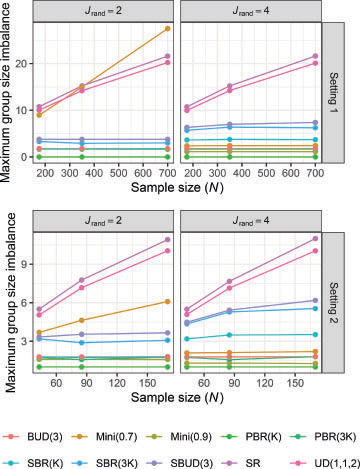
When $J_{\text{rand}}=2$, the mean maximum imbalance in the number of patients allocated to each arm for Mini(0.7) becomes much larger than its result with $J_{\text{rand}}=4$. Our findings indicate that for the smaller considered value of $J_{\text{rand}}$, Mini(0.7) performs more like SR and the UD, while it is more comparable to PBR/SBR/BUD/SBUD when $J_{\text{rand}}=4$. In contrast, Mini(0.9) has low mean maximal imbalance for both $J_{\text{rand}}=2$ and $J_{\text{rand}}=4$. This highlights the importance of careful choice of $p_{\min }$. To investigate this further, a small number of additional simulations were performed for minimization setting. They indicated, as would be expected, that the mean maximal imbalance increases as $p_{\min }$ decreases (as the procedure then functions more like SR).

3.2 Degree of Imbalance According to Patient Covariates

The simulation results comparing covariate imbalance for are displayed in Figure 2. As would be anticipated, the mean maximal covariate imbalance decreases for all methods as a function of the sample size. As many not have been anticipated, the degree of imbalance reduction as N is increased appears similar for each method.

Fig. 2 The empirical mean maximum covariate imbalance between the control arm and each of the experimental arms is shown by setting and the value of $J_{\text{rand}}$

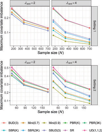
In both settings, SR, UD(1,1,2), the PBR designs, and BUD(3) have similar covariate imbalance based on our chosen metric. This is to be expected given none use covariate information in the patient allocation. For $J_{\text{rand}}=4$, Mini(0.9) is the best performing method. Mini(0.7) and SBR($K)$ are the next best methods, performing similarly. SBR(3$K)$ and SBUD(3) have slightly weaker, but still strong, performance. This indicates a large $p_{\min }$ may be necessary to outperform SBR and SBUD in some scenarios.

By contrast, for $J_{\text{rand}}=2$ we found that all considered allocation methods had similar mean maximal covariate imbalances, albeit with a small difference between randomization methods for the lowest sample size in both settings. SBUD(3) had arguably the best performance for $J_{\text{rand}}=2$. This highlights that methods which force balance on certain covariates provide no improvement in balance for other uncorrelated covariates of interest compared to simpler techniques such as SR and PBR.

To explore the influence of $p_{\min }$ on the performance of the minimization methods, Appendix, supplementary materials presents results for $J_{\text{rand}}=1, 2, 3, 4$. They indicate that, as we would anticipate, the imbalance for covariates not used in the allocation are unaffected by the value of $p_{\min }$. However, for those covariates used in the allocation, a large reduction in imbalance can be achieved by increasing $p_{\min }$. This is particularly true when $J_{\text{rand}}=1$.

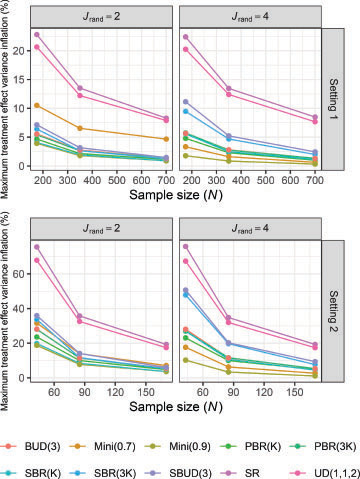
3.3 Maximal Treatment Effect Variance Inflation

The simulation results comparing the treatment effect variance inflation are displayed in Figure 3, given as empirical mean percentages. Reflecting the results in Figures 1–2, they show that the highest treatment effect variance inflation results from SR and UD(1,1,2), and that the inflation decreases as a function of the sample size. For setting 1 with $J_{\text{rand}}=2$, Mini(0.7) also performs poorly. SBR(3$K)$ and SBUD(3) are generally the next worst performing procedures. Mini(0.9) has consistently low maximum treatment effect variance inflation.

Fig. 3 The empirical mean maximum treatment effect variance inflation (given as a percentage) is shown by setting and the value of $J_{\text{Rand}}$

3.4 Predictability

Predictability of allocation is shown in Figure 4. It is clear that predictability is generally unaffected by the sample size. In Setting 1, the simulation results show that the lowest predictability results from using SR, UD(1,1,2), SBUD(3), or SBR(3$K)$. For these methods, the mean proportion of correct guesses is similar to guessing at random. By contrast, the predictability of PBR($K)$ is much higher.

Fig. 4 The empirical mean predictability is shown by setting and the value of $J_{\text{rand}}$

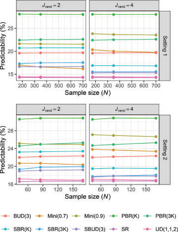
As expected, the predictability of Mini(0.7) is lower when compared to Mini(0.9). In Setting 2, notably, the predictability of Mini(0.7) is lower than PBR(3$K)$.

When $J_{\text{rand}}=2$, as opposed to $J_{\text{rand}}=4$, there was a small (3%–6%) decrease in predictability for minimization. For the SBR procedures and SBUD(3), predictability was instead lower for $J_{\text{rand}}=4$.

3.5 Power

Figure 5 displays the results for the marginal (for $H_{0,1})$, disjunctive, and conjunctive power when $J_{\text{rand}}=4$ (results for $J_{\text{rand}}=2$ are not shown but are very similar to Figure 5). As expected, all powers increase with the sample size for all allocation methods. In most cases there is evidently little difference in the resultant powers across the considered methods. The only possible exception to this is the smallest considered sample size in Setting 2.

Fig. 5 The empirical mean marginal, disjunctive, and conjunctive power are shown by setting, for $J_{\text{rand}}=4$.

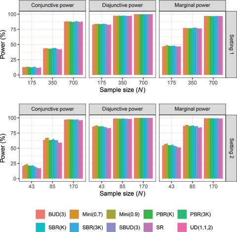
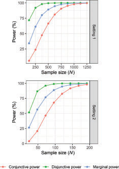
To examine whether the small observed variations in power observed in Figure 5 correspond to large changes in sample size, Figure 6 indicates how the powers vary under SR as a function of the sample size. Consider for example the marginal power in Setting 2 under Mini(0.9) when N = 85, estimated as approximately 88%. In contrast, UD(1,1,2) has the smallest marginal power, estimated as approximately 84%. Figure 6 tells us that an increase in marginal power from 84% to 88% may be considered as corresponding to an increase in sample size from approximately 86 to 96 under SR. Thus, the variations in power in Figure 5 do not represent a large change in trial total sample size.

Fig. 6 The estimated marginal, disjunctive, and conjunctive power under simple randomization is shown by setting as a function of the Trial’s total sample size.

4 Discussion

Various allocation methods have been proposed to minimize the imbalance between treatment arms according to group sizes and important patient covariates. However, there has been little consideration of their relative performance for multi-arm trials. Our study provides useful insights on this, with our results motivated by two real multi-arm trials.

The selection of an appropriate allocation method for a trial may be influenced by many factors, including the number of arms, the sample size of the trial, and the number of covariates considered. However, the goals for patient randomization in comparative clinical trials remain the same: to ensure the allocation is not predictable and to control imbalance in group sizes and according to key prognostic factors. Depending on the setting, these goals may be prioritized differently. To inform the selection of the most appropriate method, it is important to evaluate different options based on their performance.

In both settings, the best allocation methods for minimizing imbalance in the group sizes were the PBR procedures and the considered BUD (Figure 1). However, arguably there was little overall difference in the mean maximal group size imbalance when considered relative to the total sample size.

With regard to covariate imbalance, when $J_{\text{rand}}=2$, all allocation methods had similar maximal covariate imbalance in both settings, because of the two covariates not used in the allocation (Figure 2). This emphasizes an important point, discussed many times previously in the two-arm context, that SBR, SBUD, and minimization will not provide improved balance on covariates not included in the allocation routine that are uncorrelated with those included in the allocation routine. The effectiveness of SBR, SBUD, and minimization may thus be highly dependent on pretrial knowledge of which covariates may affect the outcome data.

We also highlight that using either PBR or BUD within strata (i.e., the SBR and SBUD designs) had similar, strong performance. The advantages of MTI procedures or PBR methods have been discussed extensively within the literature in relation to two-arm trials not attempting to balance for covariates (see, e.g., Berger, Bejleri, and Agnor 2016). Such advantages did not appear clear in the considered multi-arm setting with multiple strata.

We also highlight again that Mini(0.9) performed better than SBR($K)$ when $J_{\text{rand}}=4$ in terms of covariate balance. Thus, minimization can be more effective at balancing larger numbers of covariates. However, this comes at a large cost in terms of the predictability (see below and Figures 3 and 4).

Predictability of assignment provides a potential for a selection bias, which increases with a higher frequency of predictable assignments. Our simulation results demonstrate a differential effect in how the block size in the various methods has an impact on the mean predictability. Specifically, while the smaller block size increased predictability by a large amount for PBR, SBR was less effected. Significantly, the considered minimization routines had a much larger predictability than the considered SBR and SBUD routines when $J_{\text{rand}}=4$; evidencing a penalty of minimization noted above. We note though that this is for our particular definition of predictability and may not be the case if one assumes guesses are made with some knowledge of covariate data.

With regard to treatment effect variance inflation, a desirable allocation rule has low variance and a low selection bias “predictability.” However, these factors generally work against each other. As a result, the randomization rules with highest predictability typically had the lowest variances.

Despite some variation in the mean group size imbalances as well as in the covariate imbalance (Figures 1–2), our simulation results showed that the choice of allocation method did not have a major impact on the different types of power (Figure 5). The only notable differences appeared in Setting 2 due to the small assumed sample size. Thus, there is little need to consider power when choosing an allocation methodology in the considered design scenario (Wason, Stecher, and Mander 2014).

Providing a short precise summary of our findings is challenging given the volume of results and metrics considered. However, there are certain conclusions that we believe can be drawn. Evidently, the UD and SR had the highest imbalance in group sizes and covariates, causing them to have the largest treatment effect variance inflation. But they had the lowest predictability and may better balance unobserved covariates due to their increased randomness. PBR with a small block size is perhaps the most commonly used randomization method (McPherson, Campbell, and Elbourne 2012; Parmar, Carpenter, and Sydes 2014). Based solely on our considered metrics, a strong argument can be made that SBR is an overall better choice, providing the best trade off in performance overall and simplicity. The SBUD is theoretically superior, but such theoretical advantages may not outweigh the slight increased complexity in the multi-arm context unless the trial is very large in terms of both arms and strata. Despite controversy regarding the use of minimization in randomized trials (Treasure and MacRae 1998; Taves 2010), minimization was more successful in achieving a combination of group size balance and covariate balance compared to using either SBR or SBUD. Its predictability and treatment effect variance inflation were comparable to a considered PBR routine. However, its gains over SBR and SBUD may be considered insubstantial when weighed against a greatly increased predictability. A potential caveat to this statement is the dependence of the performance of minimization on the choice of parameter $p_{\min }$, though Figures 2 and 4 indicate that it would likely not be possible to find a value for $p_{\min }$ resulting in similar predictability to SBR or SBUD that retains an advantage in covariate balance.

We conclude with some limitations our work. In this article, we considered several popular randomization methods. These represent only a small subset of available methods, and examination of other methods such as maximal procedure can be considered for future work. In addition, we only considered balancing up to four binary covariates. Such categorical covariates are common in clinical trials. Even continuous covariates are typically discretized to be included in the randomization routine (Taves 2010). However, the breakdown of a continuous covariate into subcategories may lead to loss some of important information (Stigsby and Taves 2010). Therefore, there are several allocation methods that have been proposed (Su 2011; Ma and Hu 2013) to balance continuous covariates as well as categorical. Investigation of such methods within the context of multi-arm trials for allocation methods is left for further research. Moreover, we assumed all covariates impacting the outcome data were included in the final analysis model. When there is one or more unobserved covariate correlated with treatment assignment, the estimate for the treatment effect can be biased (Liu and Hu 2022). The effect of unobserved covariates on statistical inference under randomization procedures in multi-arm trials is thus also an important issue for future study. Furthermore, we considered the statistical analysis based on a continuous outcome, however, the results for other outcomes, such as binary or time to event, may differ. We also considered a statistical test based on population model assumptions. If randomization-based inference was applied instead, this could affect our conclusions. Thus, further aspects of interest include evaluation of how randomization-based inference would affect our conclusions as well as considering different types of outcomes. Furthermore, we only considered equal allocation ratios across all considered randomization methods. The choice of randomization procedure for RCTs with unequal allocation requires special additional considerations, such as the allocation ratio preserving property (Kuznetsova and Tymofyeyev 2012). Furthermore, adaptive changing of allocation ratios (i.e., (covariate) response adaptive randomization) has been increasingly commonly considered within the context of multi-arm trials (Sverdlov 2016; Park et al. 2020). The choice of adaptive randomization procedure for RCTs with unequal allocation requires special additional considerations, such as the allocation ratio preserving property (Kuznetsova and Tymofyeyev 2012). Comparison of the methods discussed here to such adaptive randomization methods is an additional potential topic for future work.

Supplementary Materials

The simulation results for the minimization method in terms of the number of covariates used in the allocation method ($J_{\text{rand}}$) and the assumed value of $p_{\min }$, can be found in Supplementary Appendix at the journal website.

Acknowledgments

The authors would like to thank the reviewers for their thoughtful comments that helped to improve the original manuscript.

Disclosure Statement

The authors have no conflicts of interest to disclose.

Additional information

Funding

This research is part of RA’s PhD studentship, funded by Umm Al-Qura University, Makkah, The Kingdom of Saudi Arabia.

References

- Atkinson, A. C. (2002), “The Comparison of Designs for Sequential Clinical Trials with Covariate Information,” Journal of the Royal Statistical Society, Series A, 165, 349–373. DOI: 10.1111/1467-985X.00564.
- Baldi Antognini, A., and Zagoraiou, M. (2011), “The Covariate-Adaptive Biased Coin Design for Balancing Clinical Trials in the Presence of Prognostic Factors,” Biometrika, 98, 519–535. DOI: 10.1093/biomet/asr021.
- Berger, V. W., Bejleri, K., and Agnor, R. (2016), “Comparing MTI Randomization Procedures to Block Randomization,” Statistics in Medicine, 35, 685–694. DOI: 10.1002/sim.6637.
- Berger, V. W., Bour, L. J., Carter, K., Chipman, J. J., Everett, C. C., Heussen, N., Hewitt, C., Hilgers, R. D., Luo, Y. A., Renteria, J., Ryeznik, Y., Sverdlov, O., and Uschner, D. (2021), “A Roadmap to Using Randomization in Clinical Trials,” BMC Medical Research Methodology, 21, 168. DOI: 10.1186/s12874-021-01303-z.
- Berger, V. W., Ivanova, A., and Knoll, M. D. (2003), “Minimizing Predictability While Retaining Balance through the Use of Less Restrictive Randomization Procedures,” Statistics in Medicine, 22, 3017–3028. DOI: 10.1002/sim.1538.
- Burant, C. F., Viswanathan, P., Marcinak, J., Cao, C., Vakilynejad, M., Xie, B., and Leifke, E. (2012), “TAK-875 versus Placebo or Glimepiride in Type 2 Diabetes Mellitus: A Phase 2, Randomised, Double-Blind, Placebo-Controlled Trial,” The Lancet, 379, 1403–1411. DOI: 10.1016/S0140-6736(11)61879-5.
- Chen, Y. P. (1999), “Biased Coin Design with Imbalance Tolerance,” Communications in Statistics. Part C: Stochastic Models, 15, 953–975. DOI: 10.1080/15326349908807570.
- Diacon, A. H., Dawson, R., von Groote-Bidlingmaier, F., Symons, G., Venter, A., Donald, P. R., van Niekerk, C., Everitt, D., Winter, H., Becker, P., Mendel, C. M., and Spigelman, M. K. (2012), “14-day Bactericidal Activity of PA-824, Bedaquiline, Pyrazinamide, and Moxifl Oxacin Combinations: A Randomised Trial,” The Lancet, 380, 986–993. DOI: 10.1016/S0140-6736(12)61080-0.
- Hu, F., Hu, Y., Ma, Z., and Rosenberger, W. F. (2014), “Adaptive Randomization for Balancing over Covariates,” WIREs Computational Statistics, 6, 288–303. DOI: 10.1002/wics.1309.
- Jin, M., Polis, A., and Hartzel, J. (2021), “Algorithms for Minimization Randomization and the Implementation with an R Package,” Communications in Statistics - Simulation and Computation, 50, 3077–3087. DOI: 10.1080/03610918.2019.1619765.
- Kernan, W. N., Viscoli, C. M., Makuch, R. W., Brass, L. M., and Horwitz, R. I. (1999), “Stratified Randomization for Clinical Trials,” Journal of Clinical Epidemiology, 52, 19–26. DOI: 10.1016/S0895-4356(98)00138-3.
- Kuznetsova, O. M., and Tymofyeyev, Y. (2012), “Preserving the Allocation Ratio at Every Allocation with Biased Coin Randomization and Minimization in Studies with Unequal Allocation,” Statistics in Medicine, 31, 701–723. DOI: 10.1002/sim.4447.
- Liu, Y., and Hu, F. (2022), “Balancing Unobserved Covariates with Covariate-Adaptive Randomized Experiments,” Journal of the American Statistical Association, 117, 875–886. DOI: 10.1080/01621459.2020.1825450.
- Ma, Z., and Hu, F. (2013), “Balancing Continuous Covariates Based on Kernel Densities,” Contemporary Clinical Trials, 34, 262–269. DOI: 10.1016/j.cct.2012.12.004.
- Matthews, J. N. (2006), Introduction to Randomized Controlled Clinical Trials, London: Chapman and Hall/CRC.
- Matts, J. P., and Lachin, J. M. (1988), “Properties of Permuted-Block Randomization in Clinical Trials,” Controlled Clinical Trials, 9, 327–344. DOI: 10.1016/0197-2456(88)90047-5.
- McPherson, G. C., Campbell, M. K., and Elbourne, D. R. (2012), “Use of Randomisation in Clinical Trials: A Survey of UK Practice,” Trials, 13, 198. DOI: 10.1186/1745-6215-13-198.
- Park, J. J., Harari, O., Dron, L., Lester, R. T., Thorlund, K., and Mills, E. J. (2020), “An Overview of Platform Trials with a Checklist for Clinical Readers,” Journal of Clinical Epidemiology, 125, 1–8. DOI: 10.1016/j.jclinepi.2020.04.025.
- Parmar, M. K., Carpenter, J., and Sydes, M. R. (2014), “More Multiarm Randomised Trials of Superiority Are Needed,” The Lancet, 384, 283–284. DOI: 10.1016/S0140-6736(14)61122-3.
- Pocock, S. J., and Simon, R. (1975), “Sequential Treatment Assignment with Balancing for Prognostic Factors in the Controlled Clinical Trial,” Biometrics, 31, 103. DOI: 10.2307/2529712.
- Ryeznik, Y., and Sverdlov, O. (2018), “A Comparative Study of Restricted Randomization Procedures for Multiarm Trials with Equal or Unequal Treatment Allocation Ratios,” Statistics in Medicine, 37, 3056–3077. DOI: 10.1002/sim.7817.
- Soares, J. F., and Wu, C. F. (1983), “Some Restricted Randomization Rules in Sequential Designs,” Communications in Statistics - Theory and Methods, 12, 2017–2034. DOI: 10.1080/03610928308828586.
- Stigsby, B., and Taves, D. R. (2010), “Rank-Minimization for Balanced Assignment of Subjects in Clinical Trials,” Contemporary Clinical Trials, 31, 147–150. DOI: 10.1016/j.cct.2009.12.001.
- Su, Z. (2011), “Balancing Multiple Baseline Characteristics in Randomized Clinical Trials,” Contemporary Clinical Trials, 32, 547–550. DOI: 10.1016/j.cct.2011.03.004.
- Sverdlov, O. (2016), “An Overview of Adaptive Randomization Designs in Clinical Trials,” in Modern Adaptive Randomized Clinical Trials: Statistical and Practical Aspects, ed. O. Sverdlov, pp. 3–44, New York: Chapman and Hall/CRC. DOI: 10.1201/b18640.
- Taves, D. R. (1962), “Minimization: A New Method of Assigning Patients to Treatment and Control Groups,” Nordisk Medicin, 67, 5–7.
- Taves, D. R. (2010), “The Use of Minimization in Clinical Trials,” Contemporary Clinical Trials, 31, 180–184. DOI: 10.1016/j.cct.2009.12.005.
- Treasure, T., and MacRae, K. D. (1998), “Minimisation: The Platinum Standard for Trials?: Randomisation Doesn’t Guarantee Similarity of Groups; Minimisation Does,” BMJ, 317, 362–363. DOI: 10.1136/bmj.317.7155.362.
- Wason, J. M. S., Stecher, L., and Mander, A. P. (2014), “Correcting for Multiple-Testing in Multi-Arm Trials: Is It Necessary and Is It Done?” Trials, 15, 364. DOI: 10.1186/1745-6215-15-364.
- Wei, L. J. (1977), “A Class of Designs for Sequential Clinical Trials,” Journal of the American Statistical Association, 72, 382–386. DOI: 10.1080/01621459.1977.10481005.
- Zhao, W. (2014), “A Better Alternative to Stratified Permuted Block Design for Subject Randomization in Clinical Trials,” Statistics in Medicine, 33, 5239–5248. DOI: 10.1002/sim.6266.
- Zhao, W., and Weng, Y. (2011), “Block Urn design - A New Randomization Algorithm for Sequential Trials with Two or More Treatments and Balanced or Unbalanced Allocation,” Contemporary Clinical Trials, 32, 953–961. DOI: 10.1016/j.cct.2011.08.004.