A novel smart steel strand based on optical-electrical co-sensing for full-process and full-scale monitoring of prestressing concrete structures

ABSTRACT

As the main load bearing component, the steel strand has a significant impact on the safety of civil infrastructure. Real-time monitoring of steel strand stress distribution throughout the damage process is an important aspect of civil infrastructure health assessment. Hence, this study proposes an optical-electrical co-sensing (OECS) smart steel strand with the DOFS and CCFPI embedded in. It can simultaneously measure small strains in the initial damage phase with high accuracy and obtain information in the large deformation phase with relatively low precision. Several experiments were carried out to test its sensing performance. It shows both DOFS and CCFPI have good linearity, repeatability and hysteresis. In comparison to DOFS, CCFPI has a relatively lower accuracy and resolution, but a large enough measurement range to tolerate the large strain in the event of a steel strand failure. To verify the reliability of the proposed smart steel strand in real structures, the strand strain distribution in the full damage process of bonded prestressed beams under four-point bending loading was monitored using the smart steel strand as a prestressing tendon. The strain measured by the OECS steel strand is shown to reflect the deformation and stiffness variation of prestressed beams under different load.

GRAPHICAL ABSTRACT

KEYWORDS:

• Distributed optical fiber sensor (DOFS)
• Coaxial cable fabry–perot interferometer (CCFPI)
• Smart steel strand
• Prestress monitoring
• Optical-electrical co-sensing

1. Introduction

Over the last 30 years, with the development of smart materials and information technology, Structural Health Monitoring (SHM) has continued to be a hot area worldwide. It has become a key method for reducing uncertainty in structural prediction models, assessing the reliability of structures and better designing new structures. Steel strands can be used as bridge cables, messenger wires, geotechnical anchor cables, cable nets and internal and external prestressing elements. In fact, as the most important load-bearing component, they have a major impact on the safety and security of civil infrastructure. The mechanical properties of the steel strands will deteriorate over time as a result of long-term stress and environmental influences. Monitoring the stress state of the steel strand in real time throughout its life cycle is therefore very important. Currently, a number of techniques have been proposed to monitor stress in the steel strand. These include vibration methods, impedance-based methods, elasto-magnetic methods, acoustoelastic methods, strain-based methods and static nondestructive testing (NDT) methods. Among them, vibration methods[[1], [2]] have low sensitivity to prestressing changes, impedance-based methods based on piezoelectric transducers [3–5] can currently only consider prestressing changes in the vicinity of the anchorage, elasto-magnetic methods [6] are not suitable for in-situ monitoring due to poor instrumentation feasibility, acoustoelastic methods [7–12] also have low sensitivity to prestressing changes and can’t monitor the distribution of prestressing along a prestressed concrete structure, static NDT methods [13] do not require direct measurement of the prestressing in the tendon, but require vertical deflections to an accuracy of 0.01 mm, which is not easy to obtain in-situ. In summary, strain-based methods [14] offer the greatest promise for monitoring prestress due to the maturity of sensing technology and the good relationship between strain and stress. Because of the relative maturing of strain-based methods in sensors and algorithms, the current research focus is on the universal implementation of strain sensors. Fiber optic sensors have been rapidly developed in recent years and are used to monitor prestress loss due to their stable sensing characteristics, high accuracy, high temperature resistance, corrosion resistance, small physical dimensions, light weight and resistance to electromagnetic interference [15-] [18]]. Optical fiber sensors were first adopted to monitor the tension of two 35-meter-long stay cables in Stork’s Bridge in Switzerland [19]. Bare fiber Bragg grating (FBG) sensors were fixed on steel strands, graphite rods and carbon fiber reinforced plastics rebars respectively to monitor the stress of prestressed tendons in six pre-stressed concrete beams of the Beddington highway bridge [20]. Gao J et al. [21] bonded Brillouin-OTDR sensors to one steel strand and three aramid fiber reinforced plastic (AFRP) cables to measure the stress of post-tensioning cables. Researchers from Harbin Institute of Technology installed 12 FBG strain sensors and 3 temperature sensors during the construction of prestressed box beam of Hulan River Bridge in Heilongjiang Province. The sensors are used to monitor the strain variation of the prestressed box beam during the tension process, and the strain increment and distribution of the box beam in the static load test [22]. Butler et al. [23] captured the early age behavior of four 11.9 m prestressed concrete bridge beams utilizing both distributed and discrete FBG arrays.

The bare fiber is made of silicon dioxide, which has a very weak shear and torsion resistance and generally need to be packaged to survive in the harsh construction and service environment of civil engineering. Zhou et al. [24–26] embedded distributed optical fiber sensor (DOFS) or fiber Bragg grating (FBG) sensors into fiber-reinforced polymer rods which were used to replace the core wire of ordinary steel strands. Thus, a new type of FRP-DOFS/FBG intelligent steel strand was proposed. It can monitor the stress state of steel strand well in the range of 75% of the proportional limit strain. But, the replacement method also provoked various problems, such as the cooperative working ability of the replaced central FRP rods and the outer steel wire under high prestress state, low mechanical properties compared with ordinary steel strand [27]. Zhu et al. [28] set a groove in the core wire of a steel strand, into which the FBG sensors can be inserted when the central wire is being stretched. This enabled the optimum range expansion of the FBG sensors with a maximum strain measurement of 12,361 με. However, the maximum total elongation of the steel strand for prestressed concrete needs to be more than 3.5% according to the correlation standard [29]. Only 30% of the maximum total elongation of the steel strand can be monitored by the optical fiber limited to its low measuring range. Local large deformation is the main cause of structural failure, and its performance is often manifested as strong nonlinear (geometric and material nonlinear) and strong coupling effect, such as bridge deck dislocation and steel cable yield under earthquake or strong wind. For the structures under extreme loads or disasters, the strain they bear can be as high as 5%-20% or even higher. Monitoring large local deformation of prestressed structures, such as bridges, is of great significance for safety assessment and maintenance decisions after suffering extreme loads or disasters. It can make people grasp the state of structural safety as soon as possible and make Bridges and other important infrastructure play their important roles in disaster relief as soon as possible. All current smart steel strands based on optical fiber have not enough measurement range to monitor the strain of the steel strand when a local large deformation occurs in the structure. Thus, they cannot assess the damage degree of the prestressed structure under extreme load loads or disasters.

This limitation is mainly determined by the material properties of low elongation of optical fiber. Coaxial cable with high elongation (strain up to 15%, more than steel yield deformation) have similar electromagnetic (EM) theory to optical fiber except for the frequency of the electromagnetic waves that travel within them, which has been greatly developed in recent years. A series of coaxial cable-based sensors have been developed including coaxial cable Bragg gratings (CCBGs) [30–33], long-period Bragg gratings (LPBGs) [34] and coaxial cable Fabry-Perot interferometer (CCFPI) [35–37]. CCFPI sensor has the advantages of small spatial resolution and adjustable gauge length, which is superior to other coaxial cable sensors [38].

The DOFS and CCFPI have good complementarity in strain measurement. The DOFS has high accuracy and small measuring range, whereas the CCFPI has large measuring range and low precision. Based on this, Jiao et al. [39] proposed an optical-electrical co-sensing tape (OECST) by encapsulating the DOFS and CCFPI sensors in a high-elastic polyurethane tape to measure the cross-sectional deformation of shield tunnels.

Given the analysis above, an optical-electrical co-sensing (OECS) smart steel strand was designed and manufactured in this paper. It can simultaneously measure small strains in the initial damage phase of a structure with high accuracy and obtain information in the large deformation phase of the structure with relatively low precision. Then, the sensing performances of the OECS smart steel strand were characterized by serious experiments. Finally, in order to verify the reliability of the proposed smart strand in real structures, the strand strain distribution in the full damage process of bonded prestressed RC beams under four-point bending loading was monitored using the smart strand as a prestressing tendon.

2. Development of OECS smart steel strand

2.1. Sensing principle of DOFS and CCFPI

2.1.1. Sensing principle of DOFS

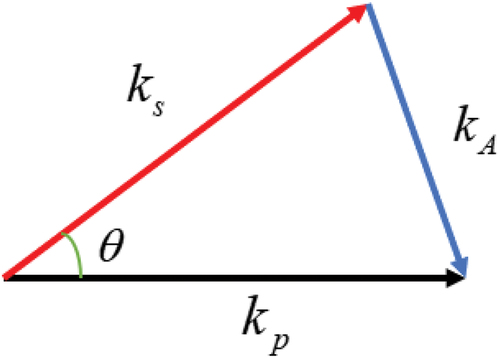
The DOFS is demodulated by Brillouin Optical Time domain Analysis (BOTDA), which is based on optical time domain reflectometry (OTDR) and stimulated Brillouin scattering (SBS). SBS can be considered in quantum mechanics as a process in which an incident photon annihilates and generates an acoustic phonon and a Stokes photon. The process satisfies the conservation law of momentum and energy, and the frequencies and wave vectors of the incident pulsed light (pump light), Stokes light, and acoustic waves can be expressed by Equation [1]:

(1) $\left\{\begin{array}{c}{\mathrm{\Omega }}_B={\omega }_p-{\omega }_s\\ k_A=k_p-k_s\end{array}\right.$(1)

Where ${\mathrm{\Omega }}_B$、${\omega }_p$、${\omega }_s$ are the frequencies of the acoustic, pump and Stokes light, respectively, and $k_A$、$k_p$、$k_s$ are the wave vectors of the acoustic, pump and Stokes light, respectively. Figure 1 illustrates the wave vector relationship between them.

Figure 1. Wave vector relation in stimulated Brillouin Scattering.

The relationship between the acoustic frequency ${\mathrm{\Omega }}_B$ and the wave vector $k_A$ is satisfied as follows:

(2) ${\mathrm{\Omega }}_B=v_A\left|k_A\right|$(2)

Where v_A is the speed at which the sound wave travels through the fiber.

Assuming $\left|k_p\right|\approx \left|k_s\right|$, this is obtained according to Figure 1:

(3) $\left|k_A\right|\approx 2\left|k_p\right|sin\frac{\theta }{2}$(3)

Substituting Equation [3] into Equation [2] gives:

(4) ${\mathrm{\Omega }}_B\approx 2v_A\left|k_p\right|sin\frac{\theta }{2}$(4)

From Equation [1], the frequency shift of the Stokes light with respect to the pump light is equal to the acoustic frequency ${\mathrm{\Omega }}_B$, i.e. the Brillouin frequency shift. Light in single-mode fibers can generally only be transmitted forward or backward, i.e. $\theta$ in Equation [4] can only be taken as 0° or 180°. Thus, the SBS produces only backward scattering, and the expression of the backward Brillouin frequency shift is shown in Equation [5]:

(5) $v_B={\mathrm{\Omega }}_B/2\pi =\frac{2n_{eff}{v}_A}{{\lambda }_p}$(5)

Where ${\lambda }_p$ is the wavelength of the pump light and $n_{eff}$ is the effective refractive index of the fiber core.

The speed of sound v_A can be expressed by Equation [6]:

(6) $v_A=\sqrt{\frac{(1-k)E}{(1+k)(1-2k)\rho }}$(6)

Where E, k and ρ are the elasticity modulus, Poisson’s ratio and density of the fiber, respectively.

Optical fibers have an elasto-optical and thermo-optical effect. Changes in strain and temperature alter the effective refractive index of the fiber core and the properties of the fiber such as Young’s modulus, Poisson’s ratio and density. From Equation [6], it can be seen that changes in strain and temperature can also lead to changes in the speed of sound in the fiber. The effective refractive index $n_{eff}$, elasticity modulus E, Poisson’s ratio k and density ρ of the optical fiber can therefore be expressed as functions of strain and temperature $n_{eff}(\epsilon ,T)$, $E(\epsilon ,T)$, $k(\epsilon ,T)$ and $\rho (\epsilon ,T)$, respectively. Then, substitute Equation [5] into Equation [6] and rewrite it as:

(7) $v_B(\epsilon ,T)=\frac{2n_{eff}(\epsilon ,T)}{{\lambda }_p}\sqrt{\frac{(1-k(\epsilon ,T))E(\epsilon ,T)}{(1+k(\epsilon ,T))(1-2k(\epsilon ,T))\rho (\epsilon ,T)}}$(7)

Assuming that the temperature of the fiber is kept constant, the effective refractive index of the fiber changes due to the elasto-optical effect when the strain on the fiber changes. Similarly, changes in the strain of the fiber will lead to corresponding changes in the elasticity modulus, Poisson’s ratio and density of the fiber. Equation [7] can be rewritten as:

(8) $v_B(\epsilon ,T_0)=\frac{2n_{eff}(\epsilon ,T_0)}{{\lambda }_p}\sqrt{\frac{(1-k(\epsilon ,T_0))E(\epsilon ,T_0)}{(1+k(\epsilon ,T_0))(1-2k(\epsilon ,T_0))\rho (\epsilon ,T_0)}}$(8)

When a very small strain is applied to the fiber, a Taylor series expansion of the above equation at $\epsilon =0$, neglecting higher order terms of 2nd order and higher, leads to a Brillouin frequency shift expression related only to the strain ε:

(9) $v_B(\epsilon ,T_0)=v_B(0,T_0)[1+(\mathrm{\Delta }{n}_{\epsilon }+\mathrm{\Delta }{\rho }_{\epsilon }+\mathrm{\Delta }{E}_{\epsilon }+\mathrm{\Delta }{k}_{\epsilon })\epsilon ]=v_B(0,T_0)(1+C_{\epsilon }\epsilon )$(9)

Similarly, the effective refractive index of the fiber changes with the temperature of the fiber due to the thermo-optical effect. Assuming that the fiber strain remains constant, the elasticity modulus, Poisson’s ratio and density of the fiber will also be affected by changes in temperature. Equation [7] can be rewritten as:

(10) $v_B({\epsilon }_0,T)=\frac{2n_{eff}({\epsilon }_0,T)}{{\lambda }_p}\sqrt{\frac{(1-k({\epsilon }_0,T))E({\epsilon }_0,T)}{(1+k({\epsilon }_0,T))(1-2k({\epsilon }_0,T))\rho ({\epsilon }_0,T)}}$(10)

The Taylor series expansion of Equation [10] at T = T₀ for small change in fiber temperature, ignoring higher order terms of 2nd order and higher, leads to a temperature-dependent Brillouin frequency shift expression only:

(11) $v_B({\epsilon }_0,T)=v_B({\epsilon }_0,T_0)[1+(\mathrm{\Delta }{n}_T+\mathrm{\Delta }{\rho }_T+\mathrm{\Delta }{E}_T+\mathrm{\Delta }{k}_T)\mathrm{\Delta }T]=v_B({\epsilon }_0,T_0)(1+C_T\mathrm{\Delta }T)$(11)

From the previous analysis of the relationship between Brillouin frequency shift and strain and temperature, it can be seen that the change of Brillouin frequency shift is proportional to the change of fiber strain and temperature. From Equations [9] and [11], the Brillouin frequency shift versus strain and temperature is given by:

(12) $v_B(\epsilon ,T)=v_B({\epsilon }_0,T_0)+C_{\epsilon }\mathrm{\Delta }\epsilon +C_T\mathrm{\Delta }T$(12)

Where Δε and ΔT are the change of strain and temperature, C_ε and C_T are strain and temperature coefficients, and $\mathrm{\Delta }{v}_B$ is the change of Brillouin frequency shift which are obtained using BOTDA.

2.1.2. Sensing principle of CCFPI [35]

As shown in Figure 2, the CCFPI sensor is essentially a coaxial cable with N (N ≥ 2) impedance discontinuities served as partial reflectors. The incident electromagnetic wave will be partially reflected at the impedance discontinuities. The two electromagnetic waves reflected at any adjacent reflectors meet each other to generate an interferogram in the spectrum domain. Assuming that the reflected electromagnetic waves at the two weak reflection points have the same frequency, the same vibrational component, the same or similar amplitude and a constant phase difference, the two reflected waves U1 and U2 can be written as:

Figure 2. The structure of CCFPI.

(13) $\left\{\begin{array}{c}{U}_1=\mathrm{\Gamma }(f)e^{-\alpha z}cos(2\pi ft)\\ U_2=\mathrm{\Gamma }(f)e^{-\alpha z}cos[2\pi f(t+\tau )],\tau =\frac{2L\sqrt{{\epsilon }_r}}{c}\end{array}\right.$(13)

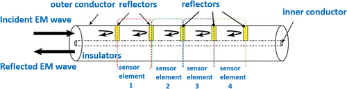
Where $\mathrm{\Gamma }(f)$ is the reflection coefficient at the reflection point, f is the frequency of the electromagnetic wave propagating in the coaxial cable, α is the propagation loss factor, z is the cable axial direction, τ is the time delay difference between the two reflected waves, L is the distance between the two reflection points, ${\epsilon }_r$is the relative dielectric constant of the dielectric material in the cable and c is the speed of light in vacuum.

The two reflected waves have a time delay difference which is related to the distance between the two reflectors and the phase speed of the wave. The interference signal U is the sum of the two reflected waves and can be written as:

(14) $U=2\mathrm{\Gamma }(f)e^{-\alpha z}cos(2\pi f\tau )cos[2\pi f(t+\tau )]$(14)

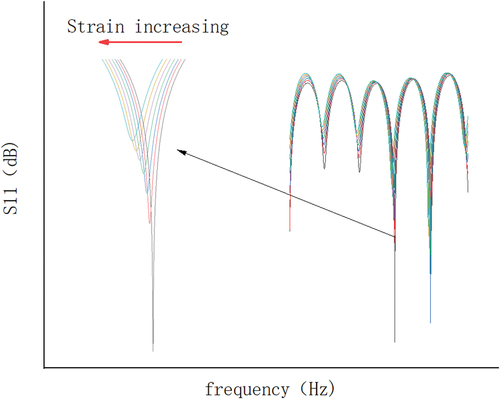
Equations [14] represents an interferometric spectrum with amplitude $2\mathrm{\Gamma }(f)e^{-\alpha z}cos(2\pi f\tau )$ and phase $2\pi f\tau$, whose amplitude and phase vary with the frequency and time delay difference. By tracking the offset of the interferogram, changes in the parameters can be detected, as shown in Figure 3.

Figure 3. The interferogram of CCFPI.

The frequency of the Nth resonant peak can be deduced from Equation [14] as:

(15) $f_N=\frac{Nc}{2L\sqrt{{\in }_r}}$(15)

Where ∈r is the relative dielectric constant of the insulating layer.

Typically, stretching of the coaxial cable leads to elongation of the cable and a reduction in the dielectric constant due to the elasto-optical effect. These are the main factors that further affect the interferogram. The strain ε can therefore be expressed in terms of the distance variation of the coaxial cable and the relative dielectric constants:

(16) $\epsilon =\frac{\mathrm{\Delta }L}{L}\begin{array}{ccc}\hspace{0.17em}& \hspace{0.17em}& \frac{\mathrm{\Delta }{\in }_r}{{\in }_r}\end{array}\simeq -P_{eff}\epsilon$(16)

Where $P_{eff}$ is the effective elasto-optical coefficient of the coaxial cable insulation.

The expression of the Nth resonant frequency shift $\mathrm{\Delta }{f}_N$ can be derived from Equations [15] and [16] as:

(17) $\mathrm{\Delta }{f}_N=\frac{\mathrm{\partial }{f}_N}{\mathrm{\partial }s}\mathrm{\Delta }s+\frac{\mathrm{\partial }{f}_N}{\mathrm{\partial }{\in }_r}\mathrm{\Delta }{\in }_r$(17)

Substituting Equation [16] into Equation [17] yields the relationship between the frequency shift $\mathrm{\Delta }{f}_N$ and the strain ε:

(18) $\mathrm{\Delta }{f}_N=f_N(\frac{P_{eff}}{2}-1)\epsilon =K_{\epsilon }\epsilon$(18)

According to Equation [18], the relationship between the resonant frequency shift and strain is linear, and the vector network analyzer (VNA) can be used to track the Nth resonant frequency shift.

2.2. The concept of optical-electrical co-sensing

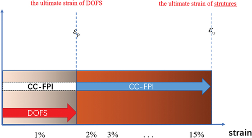
The DOFS has high accuracy but small measuring range. In contrast, the CCFPI has a relatively low accuracy but a wide range of measurement. Combining the DOFS and CCFPI for sensing can make them complement each other. In this way, optical-electrical co-sensing can not only monitor the small strain with high precision at the initiation stage of structural damage but also obtain the information of the full process of structure failure with relatively low precision.

The DOFS and CCFPI are packaged in the same matrix in parallel. When the measured structure is in the stage of small deformation, both DOFS and CCFPI can be used for strain measurement. Due to the high accuracy of DOFS, the measurements of DOFS are preferred, and the measurements of CCFPI are taken as supplements. When the measured structure develops to the stage of large deformation and the DOFS is failed, the CCFPI will take over the DOFS for the large deformation measurements subsequently. In the large deformation stage, the measurement accuracy can be appropriately reduced, and CCFPI can meet the needs of both measurement accuracy and range. Therefore, the optical-electrical co-sensing method can achieve high precision measurements in the structural initiation damage stage and relatively low precision measurements throughout the full-process of structural failure just like Figure 4.

Figure 4. Conceptual illustration of optical-electrical co-sensing method.

2.3. Fabrication of optical-electrical co-sensing smart steel strand

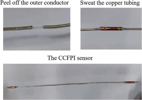
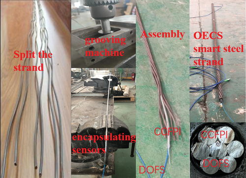
The DOFS was made of common single-mode optical fiber, and the CCFPI sensor was fabricated using SF047 coaxial cable through the cavity method as shown in Figures 5 and 6. The fabrication process of the CC-FPI sensor was as follows [1]: A section of SF047 coaxial cable was intercepted and the positions of two reflectors were marked 20 cm apart [2]; Peel off the outer conductor 6 mm at the marked position [3]; The thin-walled copper pipe with an inner diameter of 1.3 mm, a thickness of 0.1 mm and a length of 10 mm is set at the position of the reflector, then the copper pipe and the outer conductor are welded as one with solder paste.

Figure 5. Structural diagram of the CC-FPI sensor.

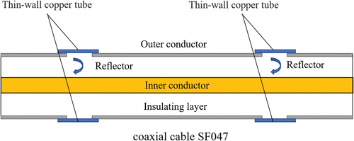
Figure 6. Fabrication process of the CC-FPI sensor.

The steel strand used is of the standard type 1 × 7, which is twisted by one central wire with a diameter of 5.2 mm and six edge wires with a diameter of 5 mm around the central wire. The nominal diameter of the steel strand is 15.2 mm, the cross-section area is 140 mm², the tensile strength is 1860 MPa, the non-proportional extension force is 234 kN, the ultimate bearing capacity is greater than or equal to 260 kN. The specific fabrication steps of the OECS smart steel strand are as follows [1]: Disassemble the ordinary steel strand and pull the core wire out [2]; Make two grooves in the core wire in longitudinal direction. One of the grooves is 0.5 mm deep and 0.7 mm wide, and the other is 1.8 mm deep and 1.8 mm wide [3]; Stretch the center wire straight, then fix one DOFS and a coaxial cable containing several cascaded CCFPI sensors in the shallow groove and deep groove with epoxy resin, respectively [4]; In order to protect the transmission parts of optical fiber and coaxial cable, both ends of the central wire are covered with armored wire tubes. Then, fill the armored wire tubes with hot melt adhesive to fix the transmission parts, as shown in Figure 7 [5]; After the epoxy resin sets, the core wire, encapsulating the DOFS and CCFPI sensors, and the edge wires are twisted to assemble into an OECS smart steel strand, as shown in Figure 9. The cross-section of the OECS smart steel strand is shown in Figure 8.

Figure 7. The armored wire tubes at both ends of the central wire.

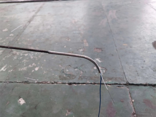
Figure 8. The schematic representation of the cross-section of the OECS smart steel strand.

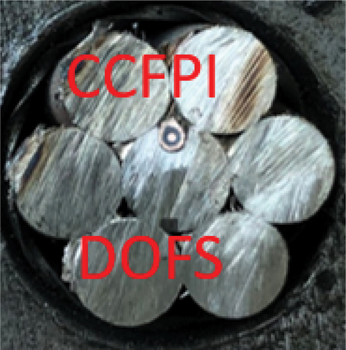
Figure 9. Fabrication process of OECS steel strand.

Due to the use of epoxy resin to encapsulate the sensor in the central wire, the long-term sensing performance of the OECS smart strand needs to take into account the effects of epoxy aging.

3. Performance of the OECS smart steel strand

3.1. Mechanical properties of the OECS steel strand

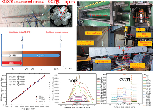
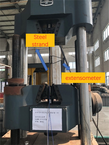
The tensile tests of the smart steel strands were carried out by using the universal material test machine as shown in Figure 10. The specimens included one standard seven-wire strand and three OECS smart steel strands. The length of the specimens were 1.1 m, the length of the fixture of the test machine was 200 mm, and the test length of the specimens was 700 mm. The specimens were uniformly stretched at a rate of 2kN/s until fracture. The force transducer and extensometer with gauge length of 100 mm of the test machine were used to measure the load and the deformation, respectively. Then, the stress strain curves of the specimens were obtained as shown in Figure 11.

Figure 10. Test of mechanical properties of steel strand.

Figure 11 shows the stress strain curves of the ordinary steel strand and the OECS smart steel strands. It can be seen from the figure that the stress strain curves of the two types steel strands show similar ductility failure trend. The elastic modulus, yield stress and maximum stress of the smart steel strands are both slightly lower than the ordinary steel strand. This is due to the slotted center wire of the smart steel strand which has smaller cross-sectional area. The main mechanical properties of the ordinary steel strand and smart steel strand are shown in Table 1. The tensile strength of the smart steel strand is 95.9% of that of the ordinary steel strand, and the elastic modulus is 95.5% of that of the ordinary steel strand, which are both close to that of the ordinary steel strand. The results show that the mechanical properties of the smart steel strand are less than 5% different from those of the ordinary steel strand. Therefore, it is expected that the OECS smart steel strand can replace the ordinary steel strand in practical engineering.

Figure 11. Stress strain curve.

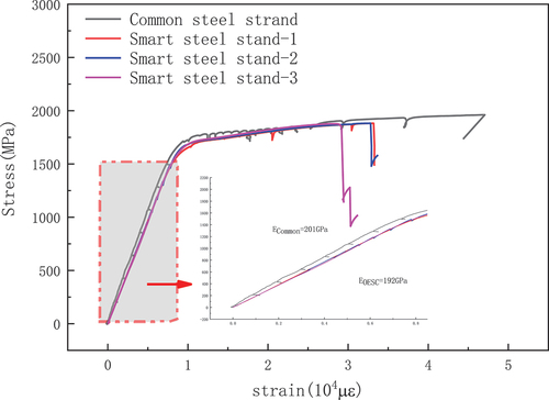
Table 1. The main mechanical properties of steel strand.

Specimen	Yield force (kN)	maximum force (kN)	Maximum elongation (%)	ultimate strength (MPa)	Elasticity modulus (GPa)
Common steel strand	246	274	4.71	1960	201
OECS steel strand	236	263	3.33	1880	192

3.2. Sensing properties

3.2.1. Linear elastic stage

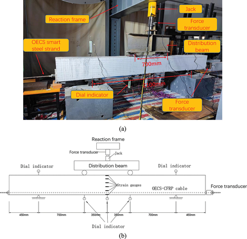
Two 2.6 m long OECS smart steel strands named S1 and S2 with three cascaded CCFPI sensors were prepared, and the experimental setup was shown as Figure 12. The gauge length of CCFPI sensors on both sides was 40 cm, and that of the CCFPI sensor in the middle was 20 cm. The spatial resolution of the BOTDA was 20 cm. An electric resistance strain gage was attached longitudinally to the outer wire in the middle of the steel strand, whose measurements serve as the true values.

Figure 12. Diagram of sensing performance experiment setup.

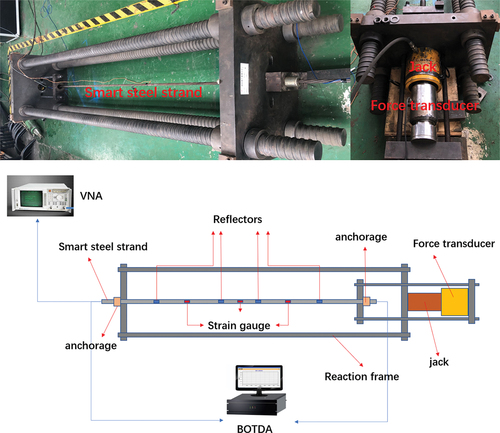
In order to evaluate the force sensing properties of the smart steel strand, three groups of cyclic loading and unloading tests were carried out. The tensile force of the smart steel strand was increased from 0 to 180 kN step by step by 30 kN, then decreased to 0 with the same loading step size. The tension was held for 5 min at each step of loading. During this time, the frequency shift of DOFS and CCFPI were acquired by BOTDA and VNA.

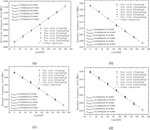
The load frequency shift curves in Figures 13 and 14 show the linear relation between load and frequency shift of DOFS and CCFPI in linear elastic stage of the smart steel strand. As shown in Figures 13(a) and 14(a), the force sensitivities of DOFS in specimen S1 vary from 1.8062 to 1.8318 MHz/kN, and the average value is 1.8120 MHz/kN. That in specimen S2 vary from 1.7221 to 1.7419 MHz/kN, and the average value is 1.7290 MHz/kN. It can be seen that the brillioun frequency shift curves have good consistency, linearity and no obvious lag.

Figure 13. Signal responses of DOFS and CCFPI in specimen S1 during loading-unloading cycles. (a) the signal response of DOFS. (b) the signal response of CCFPI-1. (c) the signal response of CCFPI-2. (d) the signal response of CCFPI-3.

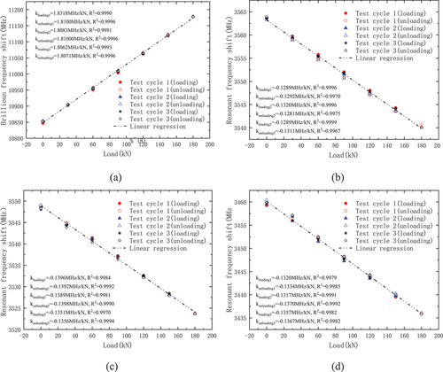
As shown in Figure 13 (b)~(d) and Figure 14 (b)~(d), the CCFPI resonant frequency shift curves of three groups of cyclic loading and unloading are in good agreement too. The high overlap of data points can be clearly observed in the plots, exhibiting a high linear response and excellent repeatability with no obvious sign of hysteresis at the end of the test. The force sensitivities of CCFPI in specimen S1 varied from 0.1281 to 0.1320 MHz/kN, 0.1351 to 0.1398 MHz/kN and 0.1317 to 0.1370 MHz/kN, respectively. The average values of which are about 0.1297 MHz/kN, 0.1380 MHz/kN and 0.1344 MHz/kN, respectively. The average force sensitivity of CCFPI in specimen S2 are about 0.1677 MHz/kN, 0.1241 MHz/kN and 0.1352 MHz/kN. The resonant frequency shift curves of CCFPI also have reasonable consistency, linearity and no obvious lag, but which are all worse than that of DOFS.

Figure 14. Signal responses of DOFS and CCFPI in specimen S2 during loading-unloading cycles. (a) the signal response of DOFS. (b) the signal response of CCFPI-1. (c) the signal response of CCFPI-2. (d) the signal response of CCFPI-3.

According to the Chinese National Standard, ‘Methods for calculating the main static performance specification of transducers’ (GB/T 18,459–2001), the main static performance indexes of the smart steel strand presented in this paper are calculated as shown as Table 2. As shown in Table 2, the maximum linearity of DOFS and CCFPI are 2.36% FS (full-scale) and 5.46% FS, the maximum hysteresis are 2.07% FS and 4.67% FS, the maximum repeatability are 1.12% FS and 3.46% FS, the maximum resolutions are 0.12kN and 1.62kN, respectively. It can be seen that the main static performance indexes of DOFS and CCFPI meet the requirements of civil engineering. Compared with CCFPI, DOFS has better linearity, hysteresis and repeatability, and higher resolution.

Table 2. The main static performance indexes of the smart steel strand.

Sensor	Linearity	Hysteresis	Repeatability	Resolution/kN
DOFS-S1	2.36%	2.07%	1.12%	0.11
DOFS-S2	1.76%	0.44%	0.85%	0.12
CCFPI-1-S1	5.46%	4.67%	2.38%	1.54
CCFPI-2-S1	3.93%	3.15%	2.41%	1.46
CCFPI-3-S1	5.35%	4.90%	3.46%	1.48
CCFPI-1-S2	4.96%	2.82%	3.08%	1.44
CCFPI-2-S2	2.64%	3.36%	2.72%	1.62
CCFPI-3-S2	4.38%	4.06%	2.51%	1.48

3.2.2. Large deformation stage

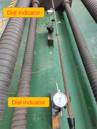
After three sets of cyclic loading and unloading tests, the full process tension damage tests of the two OECS smart steel strands were carried out to verify the whole course monitoring capability of the smart steel strands. In the test, two dial indicators were used to monitor the length change of the smart steel strand, as shown in Figure 15. The initial distance between the two dial indicator measuring points is 1000 mm, and the resolution of the dial indicators are 0.01 mm.

According to Figures 13 and 14, the tension of the smart steel strands can be calculated as follows:

(19) $F=\frac{\mathrm{\Delta }f}{k_F}$(19)

Where F is the tension of the smart steel strand, Δf is the frequency shift of DOFS or CC-FPI, k_F is the tension sensitivities of DOFS or CC-FPI.

The strain of the smart steel strand can be calculated as follows:

(20) $\epsilon =\frac{F}{EA}=\frac{\mathrm{\Delta }f}{EA{k}_F}=\frac{\mathrm{\Delta }f}{k_{\epsilon }}$(20)

Where E is the elasticity modulus of the smart steel strand, 192GPa, A is the sectional area of the smart steel strand, 140 mm², k_ε = EAk_F is the strain sensitivities of DOFS or CCFPI.

Figure 15. Deformation measurement of the OECS smart steel strand.

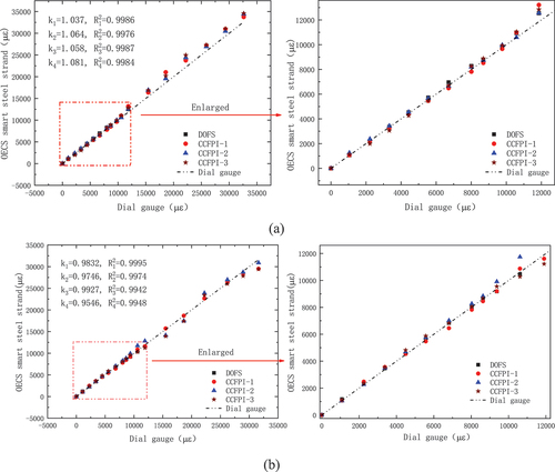
A comparison of the strain measured by the OECS smart steel strand and the dial indicator is shown in Figure 16. As can be seen from the figure that the measurement range of the DOFS in the smart steel strands is less than 12,600με, and that of the CCFPI sensors exceed the ultimate strain of the smart steel strand. The slopes of the fitting curves are all close to 1, which means the OECS smart steel strand has good strain-sensing ability throughout the whole tension damage process.

Figure 16. Comparison of the strain measured by the OECS smart steel strand and the dial indicator. (a) specimen S1; (b) specimen S2.

3.3. Prestressing monitoring methods comparison

We know that the OECS smart steel strand has the advantages of simple production, easy layout, high sensitivity of cable force perception and so on from the previous test analysis. In addition, it can monitor the strand failure stage. Table 3 compares the key features of the existing prestress monitoring methods with that of the OECS smart steel strand proposed in this paper, including spatial distribution (such as point or distributed measurement), accuracy, ambient temperature impact, cost, applicability to the prestressed reinforced concrete structure, etc.

Table 3. Comparing methods for monitoring prestressing.

Methods	Sensitivity to changes in the prestressing force	Force distribution along the structure	Accuracy	Effects of environmental temperature	cost		Applicability to the prestressed reinforced concrete structure
					sensor	Instrument
PZT-interface	High (locally)	Local but only at anchorage	Low	High	High	High	Only applicable to unbonded prestressed concrete structures
Acoustoelastic methods	Low	Not feasible, global	Medium	Not explored	None	High	Only applicable to extracorporeal prestressed concrete structure
Elasto-magnetic methods	High	Feasible, local	High	High (can be calibrated)	High	High	Only applicable to extracorporeal prestressed concrete structure
FBG sensors	High	Feasible, local	High	High (can be compensated)	High	Medium	Cable normal use phase only
DOFS	High	Feasible, Distributed	High	High (can be compensated)	Low	High	Cable normal use phase only
CC-FPI	Medium	Feasible, local	Medium	High (can be compensated)	Low	Medium	Cable normal use phase and failure stage
OECS smart steel strand	High	Feasible	High	High (can be compensated)	Low	High	Cable normal use phase and failure stage

4. Experimental study on monitoring of the bonded prestressed RC beam

4.1. Design of the bonded prestressed RC beam

An bonded prestressed RC beam with a cross-section of 200 mm × 300 mm and a span of 3000 mm was tested in this research. Figure 17(a) is the section size and reinforcement diagram of the test beam. Concrete strength grade for the test beam was C40. Four HRB400 steel reinforcements with a diameter of 10 mm were arranged in the compression zone and tension zone of the section. A metallic bellows with a diameter of 50 mm was embedded in the RC beam to serve as the prestressed channel. In order to eliminate the stress concentration of the beam, steel plates of 20 mm thickness, 120 mm × 120 mm section and spiral bars of a diameter of 6 mm, spiral inner distance of 110 mm, and five hoops were embedded in the tension and anchorage area of the beam. The mechanical properties of concrete and steel reinforcement are shown in Tables 4 and 5. A four-point bending load test on the bonded prestressed RC beam was carried out. The loading pattern and boundary conditions of the test beam are shown in Figure 17(b).

Figure 17. Cross-section of RC beam and locations of DOFS and CCFPI sensors. (a) Cross-section of RC beam; (b) Elevation view of RC beam; (c) Location of DOFS and CCFPI sensors.

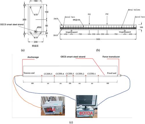
Table 4. Mechanical properties of concrete.

Age (d)	fcu,k (MPa)	fck (MPa)	Ec (MPa)	υ
28	42.2	26.9	3.26×10^4	0.31

Table 5. Mechanical properties of steel reinforcement.

Diameter (mm)	fyk (MPa)	fstk (MPa)	Es (MPa)
C10	476	644	2.10×10^5

One OECS smart steel strand proposed in Section 2.3 was passed through the prestressed channel. There were one DOFS and five CCFPI sensors along the smart steel strand, as shown in Figure 17(c). The gauge length of CCFPI sensors on both sides was 400 mm, and that of CCFPI sensor in the middle was 200 mm. A force transducer was used to measure the tension of the smart steel strand.

4.2. Tension monitoring of the smart steel strand

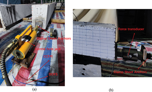
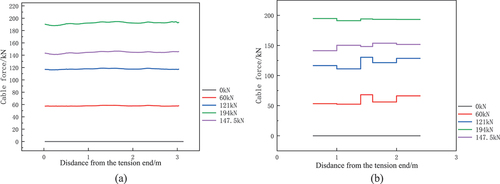
A center hole jack was used to apply the prestress to the smart steel strand of the bonded prestressed RC beam as shown in Figure 18. The tensioned and fixed ends of the steel strand are both anchored with Clip anchors. Clip anchor is a kind of anchor tool composed of clip, anchor plate and anchor cushion plate. Two or three-part clips form a pair of anchor plugs and jointly hold a strand. When the steel strand stress reached the control stress value, the jack was slowly released and the anchor clamp was brought into the conical hole of the anchor cup by the uniform retracting movement of the steel strand, forming an anchorage unit. OVM type two-hole two-part clip anchor manufactured by Liuzhou OVM Machinery Co., LTD, was selected as the anchor in this experiment. A force transducer (BLR-1) with accuracy of 0.5% FS (full-scale) and a range of 50t was mounted on the fixed end of the steel strand to measure the cable force during tensioning. The control stress was set to 1386 MPa, the corresponding tension was 194 kN. The tensile load increases in 3 steps from 0 to 194 kN, each with a load of 60 kN, 121 kN and 194 kN, respectively. The tension was held for 5 min at each step. During this time, the frequency shifts of the DOFS and CCFPI were acquired through BOTDA and VNA, as well as the cable force was measured by the force transducer. The stress in the steel strand was transferred to the test beam through the anchor cups and anchor plates to form the prestressing force. The cable force distribution along the length direction of the steel strand under different tensions is shown in Figure 19.

Figure 18. Prestress application. (a) Tension end; (b) Fixed end.

As can be seen from Figure 19, with the tension load increasing gradually, the cable force measured by DOFS and CCFPI in the steel strand also increases. In the process of prestress application, the cable force of the steel strand was roughly unchanged along the length direction of the RC beam.

Figure 19. Cable force distribution of steel strand during tension. (a) Measured by DOFS; (b) Measured by CCFPI.

A comparison of the effective prestress measured by the OECS smart steel strand and force transducer is shown in Table 6. It can be seen that the effective pretension force measured by the force transducer is 147.5 kN, and the corresponding effective prestress is 1053.6 MPa. Compared with the measurements of the force transducer, the absolute errors of the measurements of the five CCFPI sensors are respectively 44.3MPa, 20.0MPa, 5.0MPa, 44.3MPa and 30.0MPa, and the relative errors are 4.20%, 1.90%, 0.47%, 4.20% and 2.85%. The mean absolute error of all CCFPI sensor measurements is 28.7MPa, and the mean relative error is 2.72%. The absolute error of DOFS relative to the force transducer is 9.3MPa, and the relative error is 0.88%. The results show that the OECS smart steel strand can effectively monitor the effective prestress of the steel strand. In the process of prestress application, the measurement accuracy of DOFS sensor is higher than that of CCFPI sensors, so the measurements of DOFS sensor should prevail at this stage.

Table 6. Comparison of the effective prestress measurements.

Sensors	Effective pre-tensioning force (kN)	Effective prestress (MPa)	Absolute error (MPa)		Relative error (%)
CCFPI-1	141.3	1009.3	44.3	28.7 (Average value)	4.20%	2.72% (Average value)
CCFPI-2	150.3	1073.6	20.0		1.90%
CCFPI-3	148.2	1058.6	5.0		0.47%
CCFPI-4	153.7	1097.9	44.3		4.20%
CCFPI-5	151.7	1083.6	30.0		2.85%
DOFS	146.2	1044.3	9.3		0.88%
Force transducer	147.5	1053.6	0		0

4.3. Load carrying capacity calculation of the prestressed concrete beam

According to the Chinese National Standard, ‘Code for design of concrete structures’ (GB 50,010–2010), the Concrete cracking load and ultimate load of the test beam were calculated as follows.

4.3.1. Concrete cracking load calculations

The normal stress ${\sigma }_{pc}$ of the concrete produced by the prestressing force at the resultant force point of the prestressing tendons is shown in Equation [19]:

(21) ${\sigma }_{pc}=\frac{N_p}{A_n}+\frac{N_p{e}_{pn}^2}{I_n}$(21)

Where A_n is the net cross-sectional area, i.e. the sum of the total cross-sectional area of the concrete and the converted concrete cross-sectional area of the longitudinal non-prestressed tendons, N_p is the resultant force of the prestressing tendons, e_pn is the distance from the center of the net cross-section gravity to the resultant force point of the prestressing tendons, I_n is the net cross-sectional moment of inertia.

The stress increment $\mathrm{\Delta }{\sigma }_{py1}$ of the prestressing tendons from loading to concrete cracking is shown in Equation [20]:

(22) $\mathrm{\Delta }{\sigma }_{py1}=n({\sigma }_{pc}+f_{tk}\frac{e_{pn}}{y_{nb}})$(22)

Where f_tk is the standard value of the tensile strength of the concrete, n is the ratio of the elasticity modulus of the prestressing tendons to that of the concrete, y_nb is the distance from the tensile edge of the section to the gravity axis of the net section.

The stress increment$\mathrm{\Delta }{\sigma }_{c1}$of the concrete at the tensile edge of the section from the start of loading to the cracking of the concrete is shown in Equation [21]:

(23) $\mathrm{\Delta }{\sigma }_{c1}=f_{tk}+\frac{N_p}{A_n}+\frac{N_p{e}_{pn}}{I_n}{y}_{nb}$(23)

The bending moment $M_{\mathrm{c}\mathrm{l}}$ and load $P_{cl}$ when the concrete is cracked are shown in Equations [22] and [23], respectively:

(24) $M_{\mathrm{c}\mathrm{l}}=\frac{\mathrm{\Delta }{\sigma }_{\mathrm{c}1}{I}_n}{y_{nb}}+\mathrm{\Delta }{\sigma }_{py1}{A}_p{e}_{pn}$(24)

(25) $P_{cl}=\frac{4M_{cl}}{l_0-l_p}$(25)

Where l₀ is the distance between the two pivot points of the test beam, l_p is the distance between the two loading points.

4.3.2. Calculation of ultimate bearong

When the load reaches the ultimate bearing of the test beam, according to the force balance, there is:

(26) ${\alpha }_1{f}_{c}bx=f_{\mathrm{s}\mathrm{t}\mathrm{k}}{A}_s-f_{yk}^{\prime }{A}_s^{\prime }+f_{py}{A}_p$(26)

Where f_py is the ultimate strength of the prestressing tendon, $f_{yk}^{\prime }$ is the standard value of the yield strength of the compressive tendons, $f_{\mathrm{s}\mathrm{t}\mathrm{k}}$ is the standard value of the ultimate strength of the tensile tendons, $A_s$, $A_s^{\prime }$ are the cross-sectional areas of the tensile and compressive tendons respectively, $f_{ck}$ is the standard value of the compressive strength of the concrete, b is the cross-sectional width, x is the height of the compressive zone, ${\alpha }_1$ is the coefficient taken according to the specification.

The normal section ultimate bearing of the bonded prestressed concrete beam is calculated according to Equation [25] and [26]:

(27) $M_{ul}=f_{py}{A}_p\cdot (h-a_p)+f_{stk}{A}_s\cdot (h-a_s)-{\alpha }_1{f}_{c}bx\cdot \frac{x}{2}-f_{yk}^{\prime }{A}_s^{\prime }\cdot a_s^{\prime }$(27)

(28) $P_{ul}=\frac{4M_{ul}}{l_0-l_p}$(28)

According to the calculation method, combined with the reinforcement diagram in Figure 17 and the material parameters in Tables 4, 5, and the measured values of the effective prestress in Table 6, the cracking and ultimate bearing of the test beam can be obtained as 85.5 kN and 229 kN, respectively.

4.4. Loading test of the bonded prestressed RC beam

4.4.1. Test design

Once the steel strand had been tensioned, cement slurry was grouted into the prestressing apertures so that the prestressing steel strand was combined with the concrete of the beam as a whole, as shown in Figure 20. The grouting material adopted was produced by Zhongde Xinya, whose 28-day compressive strength is greater than or equal to 50MPa.

Figure 21(a) shows the actual loading setup. The total length of the RC beam was 3000 mm, the distance between the two hinge supports on both sides was 2100 mm, and the distance between the two loading points was 700 mm. One force transducer was installed between the jack and the distribution beam to measure the load in real time. In addition, another force transducer was installed at the end of the OECS smart steel strand to monitor the tension of the steel strand. Six strain gauges were uniformly arranged at midspan of the beam along the beam height direction. A total of five dial indicators were respectively arranged at the hinge supports, the midspan and two loading points of the beam. The locations of the measuring points along the beam were shown in Figure 21 (b). The strain gauges, force transducers and dial indicators were all demodulated with a sampling frequency of 1 Hz by the static stress strain test and analysis system DH3818Y.

At the beginning of loading, increased the load to 80 kN step by step by 20 kN. Then, the load was increased step by step by 10 kN until the bonded prestress beam had been completely destroyed. After that the loading mode was changed to displacement control until the midspan deflection reached 60 mm. The load was held for 5 min at each step. During this time, data acquisitions were performed.

Figure 20. Grouting of prestressed holes in bonded prestressed concrete beams.

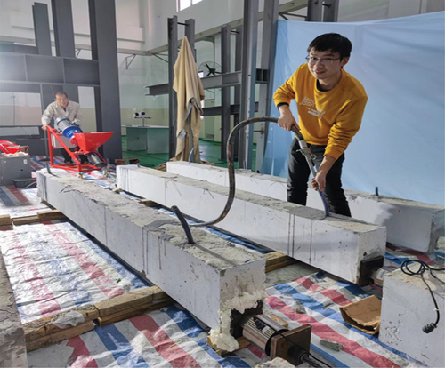
Figure 21. Setup of loading test. (a) Physical map; (b) the locations of the measuring points along the specimens.

4.4.2. Results and discussion

4.4.2.1 Cracking performance

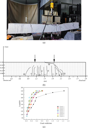
Figure 22 shows the development of cracks in the prestressed concrete beam during four-point bending load test. Figure 22(a) shows a physical view of the crack distribution of the prestressed beam at the end of the test. It can be seen from the figure that the vertical cracks in the prestressed beam were mainly concentrated in the purely bending section between the two loading points and symmetrically distributed along the midspan position. A transverse crack appeared between the midspan and the right loading point. Figure 22(b) shows the coordinates of the cracks in the prestressed beam. The crack numbers in the diagram indicate the order in which the cracks appeared. Figure 22(c) shows the variation of the width of the eight major cracks with load. As can be seen, the earliest and fastest developing crack is No. 1 near the right loading point. The Transverse crack in the prestressed beam also occured between the midspan and the right loading point. This is due to that the left support of the test beam was a sliding hinge support and the right-hand support was a fixed hinge support, which lead the test beam to translate to the left during loading and thus deflected the load to the right. It can also be seen from Figure 22(c) that the cracking load of the prestressed beam was 90 kN, and the development rate of the crack width increased rapidly after the load reached 200kN. This is due to the fact that the ordinary reinforcements in the tensile zone of the prestressed beam yielded when the load reached 200 kN and the stiffness was reduced.

Figure 22. Cracking performance. (a) Physical map; (b) the locations of the cracks along the beam; (c) Crack width development.

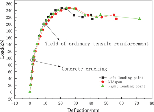
4.4.2.2 Deflection load curves

The deflection load curves for the beam at the two loading points and midspan are shown in Figure 23. The ultimate bearing of the test beam was 247 kN. Before the ultimate load was reached, the deflection increased with increasing of the load. After the ultimate load was reached, the load gradually decreased and the deflection increased rapidly. It can be seen that the slope of the deflection load curves changes abruptly at 90 kN and 200 kN. The former is the cracking load of the prestressed beam, and the latter is the load when the tensile reinforcement yielded. This is also verified by the crack width curve in Figure 22(c).

It can also be seen that the deflection at midspan is greatest, with the deflection at the right loading point being slightly greater than the deflection at the left loading point. This indicates that the deformation on the right side of the test beam is greater than that on the left side, which is also corroborated by the fact that the location of the maximum vertical crack and the transverse crack occured between the mid-span and the right loading point.

Figure 23. Load deflection curves.

4.4.2.3 Strain distribution of the smart steel strand

Figure 24(a-b)respectively shows the strain distribution of the smart steel strand measured by DOFS and CCFPI under different load. Both DOFS and CCFPI could monitor the steel strand strain until the ultimate load was reached. Once the ultimate load had been reached, the test beam entered the ductile phase where the load gradually decreased and the deformation increased rapidly. At this phase, the steel strand strain had exceeded the range of the DOFS and only the CCFPI sensor continued to monitor the strain of the steel strand. When the ultimate load was reached, the steel strand strains at midspan measured by DOFS and CCFPI were 14,094 με and 14,878 με, respectively. When the test was stopped, the load on the test beam had dropped to 214.8 kN, and the strain of the steel strand at midspan was 23,907με which was monitored by CCFPI.

Figure 24. Strain distribution of the OECS smart steel strand under different load. (a) Strain distribution measured by DOFS. (b) Strain distribution measured by CCFPI. (c) Results of midspan and loading points measured by DOFS. (d) Results of midspan and loading points measured by CCFPI.

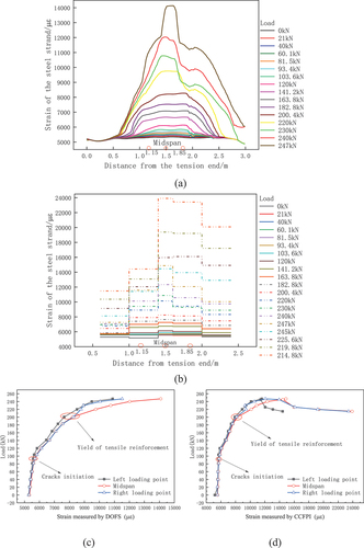
It is clear that the strain of the steel strand is greatest at the middle span, and gradually decreases from the midspan to both sides. With the load increasing gradually, the strain measured by DOFS and CCFPI sensors in the steel strand also increases. With the increase of load, the strain distribution curves of the steel strand show a tendency from dense to sparse.

From Figure 24(c) and (d), the strain of the steel strand at the midspan and loading points measured by DOFS and CCFPI increases with increasing loads. The tensile stress was borne by the steel strand, the bottom tensile reinforcements and the concrete in tension area of the test beam in the initial stage, thus the strain of the steel strand increased slowly. When the load increased to 90kN, cracks were generated in the tensile area of the pure bend section of the test beam, and the tensile stress was borne by the steel strand and the bottom tensile reinforcements. Thus, the stiffness of the test beam reduced, and the strain of the steel strand increased faster. However, when the load increased to 200 kN, the bottom tensile reinforcements yielded, and the tensile stress increment was borne by the steel strand only. Thus, its stiffness again reduced, and the strain increased faster. In addition, the strain of the steel strand at the right loading point was slightly greater than that at the left loading point. Both of these results can be verified by the cracking performance in Figure 22 and the load deflection curves in Figure 23. Which means that the strain measured by the OECS steel strand can reflect the deformation and stiffness variation of prestressed beams under different load.

The relationship between the strain of the steel strand and the flexural stiffness of the prestressed beam can be obtained by Equation [27] and [28]:

(29) $\mathrm{\Delta }{\epsilon }_p=\frac{\mathrm{\Delta }M\cdot y}{E{I}_n}=\frac{\mathrm{\Delta }P(l_0-l_p)}{K_{pc}}$(29)

(30) $K_{pc}=\frac{\mathrm{\Delta }{\epsilon }_p}{\mathrm{\Delta }P(l_0-l_p)}$(30)

Where l₀ is the distance between the two pivot points of the test beam, l_p is the distance between the two loading points, K_pc is the flexural stiffness of the prestressed beam, ΔP is the load increment of the prestressed beam, Δε_p is the strain increment of OECS smart steel strand in midspan.

5. Conclusions

This paper proposed a novel smart steel strand based on optical-electrical co-sensing for full-process and full-scale prestress monitoring of structures. Then, the sensing performance of the OECS smart steel strand was characterized by serious experiments. Finally, the OECS smart steel strand was used for the prestress monitoring of a bonded prestressed RC beam. The results show that the DOFS and CCFPI in the smart steel strand both have a good linearity of 2.36% FS and 5.46% FS, a repeatability of 1.12% FS and 3.46% FS, and a hysteresis of 2.07% FS and 4.67% FS. Compared with DOFS, CCFPI has relative lower accuracy and resolution but enough measurement range to tolerate large strain when the steel strand fail. In the loading test of the bonded prestressed RC beam, the OECS smart steel strand can effectively monitor the stress and strain distribution of the steel strand during the entire loading process. The results show that the strain measured by the OECS steel strand can reflect the deformation and stiffness variation of prestressed beams under different load.

Acknowledgments

This work was financially supported by the National Natural Science Foundation of China under Grant No. 52178282.

Disclosure statement

No potential conflict of interest was reported by the author(s).

Data availability statement

All data and models generated or used during the study appear in the published article.

Additional information

Funding

The work was supported by the National Natural Science Foundation of China [52178282].

References

- Noble D, Nogal M, Pakrashi V. The effect of prestress force magnitude and eccentricity on the natural bending frequencies of uncracked prestressed concrete beams. J Sound Vibr. 2016;365:22–44. doi: 10.1016/j.jsv.2015.11.047
- Sony S, Laventure S, Sadhu A. A literature review of next‐generation smart sensing technology in structural health monitoring. Struct Control Health Monit. 2019;26(3):e2321. doi: 10.1002/stc.2321
- Le TC, Phan TTV, Nguyen TH, et al. A low-cost prestress monitoring method for post-tensioned RC beam using piezoelectric-based smart strand. Buildings. 2021;11(10):431. doi: 10.3390/buildings11100431
- Voutetaki ME, Naoum MC, Papadopoulos NA, et al. Cracking diagnosis in fiber-reinforced concrete with synthetic fibers using piezoelectric transducers. Fibers. 2022;10(1):5. doi: 10.3390/fib10010005
- Chalioris CE, Providakis CP, Favvata MJ, et al. Experimental application of a wireless earthquake damage monitoring system (WiAMS) using PZT transducers in reinforced concrete beams. WIT Trans Built Environ. 2015;152:233–243.
- Zhang S, Zhang H, Zhou J, et al. Alternating prestress monitoring of steel strands based on the magnetoelastic inductance method. Measurement. 2022;194:111024. DOI:10.1016/j.measurement.2022.111024
- Jiao Y, Zhang Y, Shan W, et al. Damage fracture characterization of reinforced concrete beam subjected to four-point bending with parametric analysis of static, dynamic, and acoustic properties. Struct Health Monit. 2020;19(4):1202–1218. doi: 10.1177/1475921719881756
- Mpalaskas AC, Matikas TE, Aggelis DG, et al. Acoustic emission for evaluating the reinforcement effectiveness in steel fiber reinforced concrete. Applied Sciences. 2021;11(9):3850. doi: 10.3390/app11093850
- Mpalaskas AC, Aggelis DG, Matikas TE. Monitoring the fracture behavior of epoxy resin repaired fiber reinforced concrete specimens by acoustic emission[C]//sensors and smart structures technologies for civil, mechanical, and aerospace systems 2021. SPIE. 2021;11591:461–474.
- Yim J, Wang ML, Shin SW, et al. Field application of elasto-magnetic stress sensors for monitoring of cable tension force in cable-stayed bridges. Smart Struct Syst. 2013;12(3_4):465–482. doi: 10.12989/sss.2013.12.3_4.465
- Aggelis DG, Mpalaskas AC, Matikas TE. Acoustic emission signatures of damage modes in concrete. Smart Sensor Phenomena, Technol, Networks, Syst Integ 2014. 2014;9062:208–215. SPIE.
- Aggelis DG, Mpalaskas AC, Matikas TE. Acoustic monitoring for the evaluation of concrete structures and materials. In: Acoustic Emission and Related Non-Destructive Evaluation Techniques in the Fracture Mechanics of Concrete. Woodhead Publishing; 2015. pp. 269–286. DOI:10.1016/B978-1-78242-327-0.00013-1.
- Tang Y, Huang Z, Chen Z, et al. Novel visual crack width measurement based on backbone double-scale features for improved detection automation. Eng Struct. 2023;274:115158. DOI:10.1016/j.engstruct.2022.115158
- Abdel‐Jaber H, Glisic B. Monitoring of prestressing forces in prestressed concrete structures—An overview. Struct Control Health Monit. 2019;26(8):e2374. doi: 10.1002/stc.2374
- Bonopera M, Chang KC, Lee ZK. State-of-the-art review on determining prestress losses in prestressed concrete girders. Appl Sci. 2020;10(20):7257. doi: 10.3390/app10207257
- Dong Y. High-performance distributed Brillouin optical fiber sensing. Photonic Sens. 2021;11(1):69–90. doi: 10.1007/s13320-021-0616-7
- Zhang H, Zhou D, Wang B, et al. Recent progress in fast distributed Brillouin optical fiber sensing. Appl Sci. 2018;8(10):1820. doi: 10.3390/app8101820
- Yang H, Huang Y, Zhou Z, et al. Long-term performance of packaged fiber Bragg grating sensors for strain monitoring inside creep medium. Int J Smart Nano Mater. 2022;13(1):42–63. doi: 10.1080/19475411.2022.2027548
- J. Meissner, W. Nowak, V. Slowik, and T. Klink, “Strain Monitoring at a Prestressed Concrete Bridge,” in 12th International Conference on Optical Fiber Sensors, Vol. 16 of 1997 OSA Technical Digest Series (Optica Publishing Group, 1997), paper OThC1.
- Maaskant R, Alavie T, Measures RM, et al. Fiber-optic Bragg grating sensors for bridge monitoring. Cement And Concrete Composites. 1997;19(1):21–33. doi: 10.1016/S0958-9465(96)00040-6
- Gao J, Shi B, Zhang W, et al. Monitoring the stress of the post-tensioning cable using fiber optic distributed strain sensor. Measurement. 2006;39(5):420–428. doi: 10.1016/j.measurement.2005.12.002
- Ou JP, Zhou Z, Wu ZH, et al. Intelligent monitoring technology of optical fiber grating of heilongjiang hulanhe bridge[J]. J Civil Eng. 2004;(1):45–49+64.
- Butler LJ, Gibbons N, He P, et al. Evaluating the early-age behaviour of full-scale prestressed concrete beams using distributed and discrete fibre optic sensors. Construction And Building Materials. 2016;126:894–912. DOI:10.1016/j.conbuildmat.2016.09.086
- Zhou Z, Ou JP, Smart FRP-OFBG bars and their application in reinforced concrete beams[C]. Proceedings of the First International Conference on Structural Health Monitoring and Intelligent Structure, 2003, pp. 861–866.
- Zhou Z, He JP, Chen GD, et al. A smart steel strand for the evaluation of prestress loss distribution in post-tensioned concrete structures. Intell Mater Syst Struct. 2009;20(16):1901–1912. doi: 10.1177/1045389X09347021
- Lan CG, Zhou Z, Ou JP. A novel GFRP-FBG smart steel strand and its properties research. Appl Mech Mater. 2012;105:1087–1091. doi: 10.4028/www.scientific.net/AMM.105-107.1087
- Qin HY, Shen QX, Zhu WX, et al. Range‐expansion technology and fatigue performance study on the self‐sensing steel strand with an embedded fibre Bragg grating sensor. Strain. 2020;56(5):e12354. doi: 10.1111/str.12354
- Qin H, Shen Q, Ou J, et al. Long-term monitoring reliability and life prediction of fiber bragg grating-based self-sensing steel strands. Adv Civil Eng. 2020;2020:1–12. DOI:10.1155/2020/7687039
- GB/T5224-2014. Steel strand for prestressed concrete. Beijing: Standards Press of China; 2014.
- Wei T, Wu S, Huang J, et al. Coaxial cable Bragg grating. Appl Phys Lett. 2011;99(11):113517. doi: 10.1063/1.3636406
- Huang J, Wei T, Lan X, et al. Coaxial cable Bragg grating sensors for large strain measurement with high accuracy[C]. sensors and smart structures technologies for civil, mechanical, and aerospace systems 2012. Spie. 2012;8345:840–848.
- Huang J, Wei T, Wu S, et al. Coaxial cable bragg grating sensors for structural health monitoring. Int J Pavement Res Technol. 2012;5(5):338.
- Huang J, Wei T, Fan J, et al. Coaxial cable Bragg grating assisted microwave coupler. Rev Sci Instrum. 2014;85(1):014703. doi: 10.1063/1.4856695
- Stevan SL Jr, Mendes Júnior JJA, Janzen FC, et al. Long period Bragg grating in coaxial transmission lines. J Microw Optoelectron Electromagn Appl. 2015;14(1):28–39. doi: 10.1590/2179-10742015v14i1424
- Huang J, Wang T, Hua L, et al. A coaxial cable Fabry-Perot interferometer for sensing applications. Sensors. 2013;13(11):15252–15260. doi: 10.3390/s131115252
- Cheng B, Zhu W, Hua L, et al. Distributed torsion sensor based on cascaded coaxial cable Fabry–Perot interferometers. Meas SciTechnol. 2016;27(7):075103. doi: 10.1088/0957-0233/27/7/075103
- Zhu C, Gerald RE, Huang J. On the Sensitivity of Microwave Fabry–Perot Interferometers for Displacement Detection. IEEE Trans Microwave Theory Techn. 2022;70(8):3943–3953. doi: 10.1109/TMTT.2022.3183566
- Jiao T, Zhou Z, Liu J, et al. Large strain-tolerated smart steel strand with built in coaxial cable Fabry–Perot interferometer. Measurement. 2020;151:107019. doi: 10.1016/j.measurement.2019.107019
- Jiao T, Zhou Z. An optical-electrical co-sensing tape for cross-sectional deformation monitoring of shield tunnels. Tunn Undergr Space Technol. 2021;117:104148. doi: 10.1016/j.tust.2021.104148