Examining healthy food accessibility and disparity in Baton Rouge, Louisiana​​​​

ABSTRACT

Disparities in healthy food accessibility have long been a public health concern. This study used the 2-step floating catchment area method to measure healthy food accessibility in East Baton Rouge Parish, Louisiana. The research creatively integrated the population with and without private vehicle to measure spatial accessibility. The overall disparities in healthy food access were firstly exhibited by a series of weighted average accessibility under different demographic groups. Furthermore, the relationships between healthy food access and other non-spatial socio-economic characteristics were examined by ordinary least squares regression and geographically weighted regression to model the non-stationarity processes and understand the spatial variation of non-spatial socio-economic factors. The research shows that the suburb areas near the periphery of the urbanized area have the highest healthy food access; within urbanized areas, the middle-south part fares better than the rest, while the rural areas suffer from poor healthy food access. The local pockets in central city score lower than the south of the study area despite higher density of population and number of food store. Socio-economically disadvantaged population suffers from poorer accessibility because of relatively lower percentage of private vehicle ownership and they fare even worse in neighbourhoods without transit access. Such findings indicate that people are experiencing disparities in healthy food access not only because of ‘where they are’ but also ‘who they are’. These results can help planners and policymakers scientifically design strategies to improve healthy food accessibility and eliminate inequalities.

KEYWORDS:

• Spatial accessibility
• disparity
• healthy food access
• 2SFCA
• GWR

1. Introduction

Food accessibility refers to people’s ability to obtain the food providers’ services. Poor access to reasonably priced, nutritious and good-quality food may lead to poor diet with low consumption of fruits and vegetables and high consumption of energy-dense, nutritionally inferior food (Dai and Wang 2011). Low accessibility of healthy food in some geographic areas and demographic groups increases the risk of health problems such as obesity, diabetes and cardiovascular diseases (Darmon, Ferguson, and Briend 2002; Helling and Sawicki 2003; Kyle and Blair 2007; Pearce, Witten, and Bartie 2006), and has increasingly become a severe public health concern. Previous literature suggests that people with better access to providers of healthy (high-quality, fresh, low-fat and nutritious); however, affordable food, such as supermarkets and fruit and vegetable markets, tend to have healthier diets and lower levels of obesity (Zenk et al. 2006). With the growing health concern for adolescents, children and adults in the United States and other countries, the issue of food desert, as well as the influence of neighbourhood food environment on human health, has been widely discussed in the literature (Michimi and Wimberly 2010).

The term ‘food desert’ refers to an area characterized by relatively poor access to healthy and affordable food. It may contribute to social disparities in diet and diet-related health outcomes (Wrigley 2002). While the research of food desert focuses on the insufficiency of food providers in a defined area, its natural extension examines the healthy and affordable food accessibility difference between socio-economically advantaged and disadvantaged areas and population group (Beaulac, Kristjansson, and Cummins 2009). These spatial accessibility barriers are often linked to and interact with non-spatial factors such as race and poverty issues, partly because of people with specific ages and income have limited mobility, and partly because uneven geographic distributions of providers and consumers force people to travel far away to purchase healthy food (Wang and Luo 2005).

To properly demonstrate the local healthy food environment, the choice of accessibility measure is essential since accessibility is a function of the indicators used (Talen and Anselin 1998; Talen 1998). The Risk Factor Monitoring and Methods Branch at the National Cancer Institute (http://epi.grants.cancer.gov/mfe/categorizing-the-food-environment) recommends two simple measures of accessibility – the nearest distance to food stores in order to evaluate immediate proximity, and counts of the number of food stores within a specific area, to evaluate the richness of food providers for cities and towns across the United States. While these two methods capture some intuitional characteristics of local food environment, they neither consider customer’s choice of food retail nor population’s share of food store capacity. A number of studies in the United States have asserted that people in rural (Kaufman 1999; Morton and Blanchard 2007; Powell et al. 2007; Sharkey and Horel 2008), low-income (Baker et al. 2006; Jetter and Cassady 2006; Morland, Roux, and Wing 2006; Powell et al. 2007; Zenk et al. 2006) and minority-concentrated (Morland and Filomena 2007; Powell et al. 2007) residential communities are most affected by food access inequalities. One major reason is that people in these areas experience more competition for food as the population density is high and/or supermarkets and quality grocery stores with healthy food are few.

Accounting for consumers’ choices and population’s share of food store capacity, many existing studies (Michimi and Wimberly 2010) use a measure that calculates the ratio of the number of food providers to population within an administrative unit, or a defined area within a fixed range from a residential area by the floating catchment area method. Although this method is straightforward and considers the match ratio between population and food resources, it comes short in capturing the spatial interaction between them. Specifically, it ignores two aspects in interaction across boundaries of residential areas: competition for food stores from adjacent neighbourhoods and competition for customers from food stores in nearby residential units (Dai and Wang 2011). Luo and Wang (2003) developed the popular 2-step floating catchment area (2SFCA) method to measure spatial accessibility by accounting for the match ratio between supply and demand and possible spatial interaction beyond boundaries of analysis units.

When measuring food accessibility, most of the literature did not separate the population by mobility, or availability to private vehicles. However, walking or taking the public transit would be the only choice that carless population has to rely on for food purchasing. Such part of population, although composes only small portion of the total, should not be neglected since their limited mobility may force them to choose unhealthy diets and turn them into the major force of some health problems like obesity. Regarding transit system’s role, pioneering research was conducted by Farber, Morang and Widener (2014) and Widener et al. (2015) to measure food accessibility in Cincinnati, Ohio based on transit network focusing on the carless population. However, their research only focuses on the carless population and neglects the comparison between the car-owning and the carless population that can reveal how access to food store can be deprived because not owning a private vehicle. It is also necessary to have an integral view of overall food-retailing environment for both car-owning and carless population groups.

Food accessibility varies across spatial and non-spatial dimensions. Many studies identified the relationships between food accessibility and spatial/non-spatial variables, which include, but are not limited to mobility, distance, social capital and economic and behavioural factors (i.e. preference for convenient food) (Widener, Metcalf, and Yaneer 2013). Some researchers focus on spatial factors such as urban versus rural areas, drawing the conclusion that rural areas are under the risk to become food desert (Morton and Blanchard 2007). Others emphasize non-spatial factors such as income and ethnicity (Powell et al. 2007). On a national scale of the United States, low-income neighbourhoods’ availability to chain supermarkets is 25% lower than mid-income neighbourhoods. In terms of ethnicity, the white neighbourhoods enjoy twice the availability as the African-American neighbourhoods, while the Hispanic communities have only one-third availability as those are not. Since food accessibility is intrinsically a ‘spatial’ problem, spatial autocorrelation may exist in the variables and influence the analysis results. Thus, particular spatial statistics methods are needed to better quantify the spatial effects. Dai and Wang (2011) used the spatial lag model to control the spatial autocorrelation effects of the food accessibility and socio-economic indices in South-west Mississippi. From the ordinary least squares (OLS) regression and spatial lag regression results, they concluded that low food accessibility in the rural areas was the result of geographic impedance rather than socio-economic and demographic characteristics, while in urban areas, lack of mobility and impaired financial status mainly contributed to poor access. This is an early attempt to account for spatial autocorrelation effects by using spatial regression techniques in modelling spatial accessibility and socio-economic factors. The obvious next step is to apply other spatial statistic methods such as spatial filtering (Griffith and Peres-Neto 2006) or geographically weighted regression (GWR) (Fotheringham, Brunsdon, and Charlton 2002; Zhao et al. 2016) to further examine how spatial effects influence the relationships between spatial accessibility and socio-economic factors. Of particular interest in this research, GWR has the advantages to model the spatial non-stationarity processes as well as understand the local effects from individual socio-economic factors to the spatial accessibility.

Based on the literature review above, the major contributions of this study include: (1) we integrated both scenarios of population with and without private vehicles when measuring healthy food accessibility, with the utilization of public transit incorporated for the carless scenario; (2) we explored both spatial and non-spatial disparities in healthy food access by using GWR. Considering that the scope of this study is not to examine or develop new accessibility metrics, we adopt the original 2SFCA method developed by Luo and Wang (2003) to measure the healthy food accessibility in East Baton Rouge Parish, Louisiana. The results from the research will help policymakers and urban planners scientifically design healthy food access strategies and eliminate dietary barriers.

2. Study area and data

2.1. Study area

This research selects East Baton Rouge Parish as the study area. A parish is a county-equivalent unit in Louisiana. The City of Baton Rouge is the parish seat of East Baton Rouge Parish with the largest area and population. In order to account for possible edge effect (i.e. interaction between consumers and food resource beyond the parish boarder), the study area is expanded by a 25-min driving distance – the travel time threshold discussed in Section 3.3 – buffer zone around East Baton Rouge Parish to include the population demand, food stores and road network in adjacent cities. The study area includes the whole spectrum of urban, suburb and rural areas.

2.2. Demographic and socio-economic data

The census data at the block group level are obtained from the 2010–2014 American Community Survey 5-Year Estimates (https://www.census.gov/geo/maps-data/data/tiger-data.html). This study is based primarily on the block group level because it is the smallest census unit with socio-demographic variables needed for the analysis such as race/ethnicity, gender, housing status, family structure, income, education, employment and an important variable: private vehicle availability. The block group-based data also can well reflect the patterns of social interaction that evolve with street and road networks (Grannis 1998).

There are 302 resided block groups in the study area consisting a population of 439,662 in 2014. Figure 1 shows that the highest population density is around the city centre and the population density gradually decreases as the distance from the city centre increases. The un-resided area in the middle-north part of the study area, donated by the black–white shade, is the Baton Rouge Airport. Population-weighted mean centre is used as the centroid for each block group to represent its location more accurately. As suggested by Hwang and Rollow (2000), the population centroid would provide more accurate estimate in trip distance or travel time between areal unit comparing with the geometric centroid.

Figure 1. Population density in block groups of East Baton Rouge Parish.

2.3. Food store classification

The food store data with geographic coordinates are gathered from the Reference U.S.A. database service (http://www.referenceusa.com/). According to the categorization defined by the National Cancer Institute, the ‘food store environment’ consists of grocery stores, supermarkets, convenience stores, snack bars, specialty food stores, farmer’s markets, bodegas and food banks. After a field survey for all recorded stores, convenience stores, snack bars, bodegas and food banks are excluded from analysis, as this study treats food store selling fresh goods as healthy food retail. There are 227 remaining healthy food retails within the study area and its extension. In a study conducted by Breza and Liberman (2017), the business capacity of the food store could be represented by the logarithm of food retail’s sales volume. We adopted this measure as the service capacity of healthy food store.

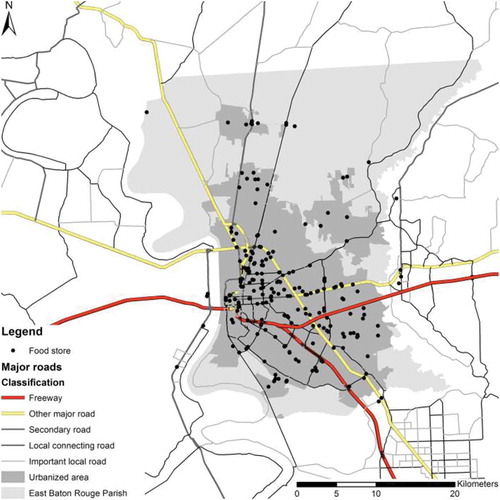
Figure 2 shows the distribution of food stores as well as the urbanized area in the East Baton Rouge Parish. The vast majority of the food stores are located inside the urbanized areas, especially the southern part of the study area – the City of Baton Rouge.

Figure 2. Food store locations.

2.4. Road and public transit network

The road network data set is originally from the 2012 Esri Streetmap data set (http://www.esri.com/data/streetmap) that includes all levels of roads and streets with essential information such as speed limits and directions. People without access to private vehicles may walk or utilize the public transit system to purchase food. Figure 3 shows the study area’s transit system, provided by Baton Rouge’s Capital Area Transit System (http://www.brcats.com/). The transit system majorly operates in the urban area. The measure of spatial impedance is the shortest vehicular travel time through the road network by following the speed limits. The comfortable walking speed for a healthy human is set at approximately 4.68 km/h (Bohannon 1997; Nishimori and Ito 2014). For people relying on the public transit system, the total travel time is approximated as the network travel time on the transit network.

Figure 3. Transit routes in Baton Rouge.

3. Methods

3.1. Estimating population with and without vehicle

The accessibility measure differs between the population groups with private vehicles and those without. Denoted by , the population without access to private vehicles at residential site is approximated as:

(1)

where is the ratio of the number of households that do not own a private vehicle, , to the total number of households at block group , ; and is the total population within that block group. From the census data discussed in study area and data section, and at the household level are available but at the individual level is not available. The above approximation assumes that each individual block group has a uniform household size within it.

Obviously, the population with access to vehicles, is estimated as:

(2)

Based on Equations (1) and (2), Figure 4 shows the distribution of population without access to a private vehicle. The overall carless percentage is 7.249% but the neighbourhoods in the central city are facing major lack of private vehicles – as high as 47.3%.

Figure 4. Percentage of population without private vehicles.

3.2. Measuring spatial accessibility – 2SFCA method

The 2SFCA method was first developed by Luo and Wang in 2003 and was utilized in this research. The details of this method are illustrated as follows (Luo and Wang 2003):

First, for each food store (supply location), search all block group centroids (demand locations) that are within a travel time threshold from the food store location to form a catchment area, and sum the total population within the catchment area up as the availability for this food store . Then compute the store-to-population (supply-to-demand) ratio within each catchment area to measure the availability of each store:

(3)

where is the total demanding population of the block group whose centroid falls into the catchment area of the store (); is the travel time between the store and each block group while is the aforementioned travel time threshold; is the capacity score for the store .

Next, for each block group , search all food stores that are within the same travel time threshold as in the first step and sum up again the store-to-population ratio to obtain the accessibility at the block group:

(4)

where is the availability of stores that fall into the catchment area of the block group ; is the travel time between block group and the store .

With population separated by mobility, the population served by stores should be calculated separately. The availability of food store in Equation (6) is updated as:

(5)

Similarly, food stores’ accessibility of each block group should be the weighted average of accessibility of both population groups in the block group:

(6)

3.3. Defining travel time threshold

In the above formulations for spatial accessibility, it is critical to define the threshold travel time . According to Hamrick and Hopkins (2012), the mean value for an average urban American’s driving time to grocery store is approximately 15 min, while it is 25 min averagely for rural residents, according to a survey conducted by Smith et al. (2010). So this study sets the threshold travel time by personal vehicle as 15 min for urbanized areas, and 25 min for rural areas. For walking, Yang and Roux (2012) suggested a 15-min range for everyday purposes, which is adopted as for this study.

For consumers that rely on public transits, a food-purchasing trip is composed of walking between house/store and transit stop and outbound/inbound transit ride, in substitution of walking. According to a study about the walking distance to light-rail stations (O’Sullivan and Morrall 1996), the preferred walking distance threshold is suggested as 326 m. Inside and outside the study area, 254 block groups (out of 359) and 111 food stores (out of 227) are beyond this threshold from any transit stations, and are thus considered inaccessible and excluded from our transit analysis. The bus-riding time is computed similarly to the travel time by private vehicle. The walking time from and to bus stops is not incorporated in the total travel time since measuring the precise travel time is beyond the scope of this study. The bus-riding time threshold for one-way trips was also set at 15 min.

4. Results

4.1. Spatial accessibility to healthy food

Figure 5 shows the map of standardized accessibility scores by the 2SFCA model for population with private vehicles and those without, respectively. The scores are normalized to a scale of 0–100 for convenience to compare.

Figure 5. Spatial accessibility for different scenarios: (a) with vehicles and (b) without vehicles.

Because the travel time threshold is greater in rural areas, the accessibility score of rural neighbourhoods adjacent to urbanized areas (suburb areas) is the highest. Within urbanized area, the neighbourhoods in the middle-south area enjoy the best access to healthy food in the study area, while those in the central city with the densest population do not fare as good since large food stores and chain supermarkets tend to be located in areas with lower land price, better transportation and higher median household income. The real rural areas distant from urbanized areas have the poorest access to healthy food. Above is for the scenario through car-travelling. For the small yet significant portion of population without private vehicle, they only have limited access (lower than 60) in limited areas (in and around central city). Those who neither have access to a private vehicle nor public transit fare even worse.

The overall accessibility is mapped in Figure 6 using Equation (5). The distribution of accessibility scores shows a sectional pattern: low healthy food accessibility is pervasive in the north-eastern rural areas; the central city only has mediocre access to healthy food, while the suburb areas around urbanized areas and the middle-south part enjoys better. This sectional pattern is​​​​ similar to the driving scenario shown in Figure 5(a) because population without access to private only accounts for a small percentage, as discussed in Section 3.1. The pattern of healthy food accessibility largely coincides with the distribution of food store.

Figure 6. Healthy food accessibility in Baton Rouge.

4.2. Ordinary least squares regression analysis

To better understand the potential relationships between healthy food accessibility and socio-economic factors, the OLS regression was used to examine such relationships. Based on previous literatures (Baker et al. 2006; Dai and Wang 2011), eight socio-economic variables are selected and their descriptive statistics are reported in Table 1.

Table 1. Descriptive statistics of accessibility and socio-economic factors.

Variable	Abbreviation	Minimum	Maximum	Average	Standard deviation
Dependent variable
Accessibility		5.749	98.588	46.514	13.152
Independent variable
Female–male ratio	Gender	0.504	2.969	1.141	0.362
Non-white (%)	Race	2.020	100	55.280	34.610
Divorce (%)	Divorce	0	48.903	11.904	7.920
Female householder (%)	Householder	0	74.255	19.943	15.019
Poverty rate (%)	Poverty	0	87.294	19.055	16.757
No high school diploma (%)	Education	0	50	13.872	11.987
Unemployment rate (%)	Job	7.246	74.286	33.376	11.192
Renter-occupied housing (%)	Renter	0	100	38.090	27.220

The initial assessment adopted OLS regression to analyse the relationship between the spatial accessibility scores and demographic/socio-economic variables within the whole study area. Spatial accessibility metrics from 2SFCA model are used as dependent variables in the OLS regression analysis. After the stepwise model selection process, variables including poverty rate, unemployment rate and renter-occupied housing percentage are chosen to use in the OLS regression analysis. Table 2 shows the OLS regression analysis results.

Table 2. OLS regression analysis results (2SFCA model).

Parameter	Parameter estimate	Standard error	t-value	p-value	VIF
Intercept	40.498	2.749	14.729	0	–
Poverty	−0.123	0.066	−1.877	0.062	2.14
Job	0.130	0.073	1.779	0.076	1.18
Renter	0.104	0.038	2.680	0.008	1.99

Adjusted  = 0.017, p-value < 0.1, AICc = 2414.187.

The regression analysis results indicate that lower accessibility scores tend to be associated with higher rate of poverty and unemployment indicates lower healthy food access. Neighbourhoods with higher percentage of renter-occupied housing have higher health food access. These results give us a general idea about how socio-economic factors influence the spatial food accessibility in our study area.

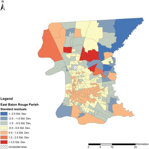
The map of OLS regression standard residuals (Figure 7) shows a noticeable spatial autocorrelation exists in the study area. The global Moran’s I is 0.164 with a standard normal z-score of 17.692 (p = 0.000), indicating that a clustered pattern of standard residuals is found.

Figure 7. Standard residuals from OLS model.

4.3. Geographically weighted regression

To eliminate spatial autocorrelation and better understand the local effects of socio-demographic factors to spatial accessibility, GWR was applied to further calibrate the regression model. GWR is a local statistical modelling method to explore and analyse the spatially varying relationships (Fotheringham, Brunsdon, and Charlton 2002). It releases the underlying spatial stationarity assumption of the OLS regression to spatial non-stationarity. More details on the mechanics of GWR are beyond the scope of this paper and are provided elsewhere (e.g. Fotheringham, Brunsdon, and Charlton 2002). Same independent variables in the OLS regression analysis were used in the GWR analysis in GWR 4.09 software. We used adaptive bi-square kernel as the geographic kernel and golden section search for optimal bandwidth search. Euclidean distance was utilized to measure the optimal bandwidth. Corrected Akaike Information Criterion (AICc) was applied as the criterion for finding optimal bandwidth.

Table 3 shows the GWR results. The optimal bandwidth is 70 nearest neighbours. The adjusted R-squared increases from 0.014 to 0.326 and the AICc decreases from 2414.187 (OLS) to 2331.281 (GWR), which means the model captures spatial effects and has a better model fit.

Table 3. GWR analysis results.

Parameter	Mean	Minimum	Lower quartile	Median	Upper quartile	Maximum
Intercept	46.996	16.669	35.516	49.643	58.684	67.184
Poverty	−0.134	−1.383	−0.200	−0.095	−0.040	0.293
Job	0.066	−0.224	−0.110	0.039	0.210	0.565
Renter	0.047	−0.182	−0.049	0.003	0.094	1.048

Adjusted  = 0.326; AICc = 2331.281. Optimal bandwidth size = 70 (nearest neighbours).

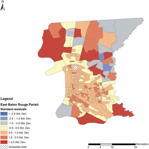
Figure 8 shows the standard residual maps of the GWR model. The global Moran’s I is 0.010 with a standard normal z-score of 1.434 (p = 0.151). Given the results above, the pattern of standard residuals of GWR does not appear to be significantly different from random. A significant improvement of spatial autocorrelation effects is achieved by using GWR.

Figure 8. Standard residuals from GWR model.

The local map of the GWR analysis is shown in Figure 9(a). The demographic and socio-economic statuses can explain more variance of spatial accessibility with a higher R-squared in the southern part of the study area.

Figure 9. ​​​​GWR model fit and parameter estimate: (a) Local R-squared of the GWR model; (b) Parameter estimate for poverty rate; (c) Parameter estimate for unemployment rate; (d) Parameter estimate for renter-occupied percentage.

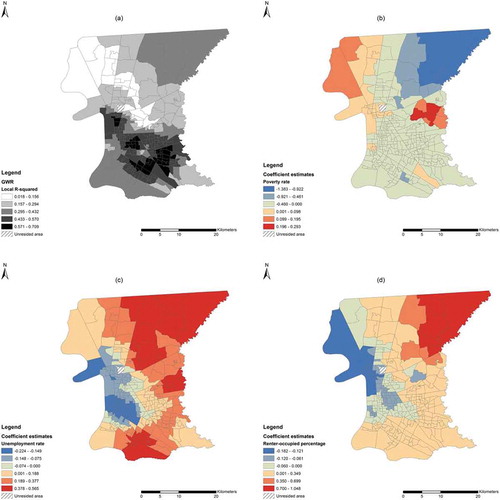
To better understand the GWR analysis results and explain the phenomenon, parameter estimate figures are mapped in Figure 9(b–d) above. The local parameter estimate of GWR analysis varies across the study area but showed some interesting twists comparing to the OLS regression model.

The global estimate of poverty rate is −0.123, meaning that neighbourhoods with more severe poverty situation may also suffer from poorer accessibility to healthy food. The GWR results (Figure 9(b)) also support such indication across the vast majority of the study area with all negative parameter estimates in the study area. Further, a higher poverty rate may matter even more in the north-eastern rural part of the study area. The direct cause of such trend is few of the decent healthy food retails located in the central city. But intrinsically, this phenomenon happens because of the disadvantages in socio-economic environment: high land price, low income, lack of awareness of healthy diet and high crime rate. All of these factors keep quality food retail away from these areas.

Globally, neighbourhood with higher unemployment rate tends to have higher healthy food access, as the global estimate of 0.130 suggests. All non-central city urban neighbourhoods, suburbs and rural areas remain consistent with the global trend, as shown in Figure 9(c). However, such advantageous trend in areas outside the central city may not necessarily be translated into true advantage in accessing healthy food, as the socio-economic disadvantages that limit consumer’s mobility and affordability remain as a major obstacle. However, areas in and around central city have inverse trend: a neighbourhood with lower percentage of employment may indicate even worse access. Similar reasoning could be drawn that higher unemployment rate may cause multiple disadvantages in socio-economic environment mentioned previously that could drive healthy food retail business away.

The parameter estimates of renter-occupied housing percentage, shown in Figure 9(d), show a concentric pattern that it is negatively correlated to the healthy food accessibility in eastern part of the study area while positively westwards. So despite a global estimate of 0.104, a higher renter-occupied housing percentage in the east may suggest that this area has lower healthy food access. However, such relation reverses in the vast non-central parts of the study area.

5. Discussion

The results of the spatial accessibility to healthy food for two mobility scenarios as well as the overall accessibility map clearly reveal the fact that the spatial disparity exists among urban and rural areas: suburb areas adjacent to the periphery of the urbanized area have the best access to healthy food; inside the urbanized areas, the middle-south part enjoys significantly better access, while people living in rural areas have no choice but to travel long for reliable healthy food retail. Such trend of distribution is reasonable since it is the nature of business to choose the urban areas, which constitutes over 80% of population in merely 30% of the study area, to ensure the retail income. So spatial disadvantage, or ‘where they are’, can be a factor that limits accessibility.

However, the spatial disadvantage (i.e. being in urbanized area or suburb and rural area) is not the only implication of a neighbourhood’s accessibility to healthy food. In fact, residents living in the city centre do not enjoy as enough food access as those in other parts of the urbanized areas. The OLS regression analysis suggests that the differences in socio-economic and demographic statuses are the primary non-spatial indicators of disparities in healthy food access. Ethnicity does not have a significant correlation with accessibility to healthy food because the higher travel time threshold outside of the central city mitigated the effect of long travel distance. The economically disadvantaged (in terms of poverty rate and unemployment rate) neighbourhoods suffer from poorer access. Such areas being not preferable for large food stores could be one reason. But more importantly, the disadvantage in economic status would result in low ownership of private vehicles, which more directly impacts spatial accessibility – local pockets in central city suffer from the relatively lower percentage of private vehicle ownership. Because of the service of public transit, the healthy food access for residents alongside the transit route is enhanced to some extent. But for those without convenient access to public transit service, they have to experience double ‘handicaps’ and fare even worse. It is easily understandable that neighbourhoods primarily occupied by renters, except for the east of the study area, have a clear advantage in healthy food access because such convenience is an essential selling point for leasing businesses.

Recent literature suggests that the linkage between built environment and obesity prevalence varies a great deal across geographic settings, and some built environment factors such as street connectivity and walkability seem to be only relevant in influencing physical activity and obesity risk in suburban areas but not in central city or rural areas (Xu and Wang 2014). Our research proves that spatial accessibility is not the only factor to limit the food access of the urban poor, bad socio-economic conditions exacerbate the limitation of food accessibility. Socio-economic conditions can heavily influence people’s dietary habit – disadvantaged people may have no choice but to purchase energy-dense, nutritionally inferior but cheap food, even with sufficient healthy food supply around their neighbourhoods (Helling and Sawicki 2003; Larson, Story, and Nelson 2009). On the other hand, healthy food retails would prefer to extend their businesses in urbanized areas with more convenience in commuting and better financed neighbourhoods since their target customers are supposed to spend more on the choice of food to ensure physical health. That is to say, a region’s socio-economic characteristic can shape the choice of location of healthy food retail, thus eventually influencing the region’s access to healthy food. Hence, healthy food access remains an issue for socio-economically underprivileged groups, not only because of ‘where they are’ but also possibly ‘who they are’ such as their affordability to constantly consuming healthy food, or how much they tend to emphasize the importance of healthy food to remain healthy in everyday life. In other words, from a public policy perspective, the focus should be not only on the spatial aspect of ‘food desert’ but also on the non-spatial dimensions.

The Economic Research Service of USDA (http://www.ers.usda.gov/data-products/food-access-research-atlas/go-to-the-atlas.aspx) also provides a ‘Food Access Research Map’ at census tract level based on distance to the supermarkets. Comparing with USDA’s national map, this research returned more detailed spatial variation of local food access in a more intuitionistic way. This research also complemented major urban, suburb and rural areas that the national map does not cover.

6. Conclusions

This study used the 2SFCA method to measure the healthy food accessibility in East Baton Rouge Parish, Louisiana with the disadvantaged population taken into special consideration by separating population according to the mobility (availability to private vehicles) and measured the spatial accessibility for both scenarios. This study further examined the disparities of healthy food access on demographic and socio-economic dimensions by using OLS regression and GWR. Our research suggests that the spatial accessibility tied to one’s location is not the only barrier that prevents the urban poor from obtaining and developing a healthy diet. What matters more is the complex interaction among socio-economic attributes, spatial accessibility and consumer mobility and behaviour.

Examining and mitigating disparities to public services have always been of great interest to urban planners and public policy analysts. In this case, for example, efforts might need to be focused on enhancing carless population’s mobility, such as frequenting public transit services that connect certain neighbourhoods and large food stores. Setting up more bike lanes and pedestrians’ walkways would be another approach to encourage those people to purchase healthy food instead of consuming fast food. In addition to food access, public services may also include healthcare facilities (Wang and Luo 2005), public green spaces (Irvine et al. 2009), public transportation (Murray et al. 1998) and digital resource (Driskell and Wang 2009). Any meaningful planning or policy design begins with scientific assessment of the disparities for access to such a service.

Future research may be advanced in several directions. Farber, Morang and Widener (2014) assessed food accessibility in a temporally dynamic way by investigating variations in accessibility across the day. An interesting method to model transit travel time is proposed by Widener et al. (2015) where they considered an option that people can make grocery stops on their way home from work based on transit travel time. Some technical details could also be further developed. To name a few, first, food store scores can be assigned according to more detailed quality, quantity and price information from food survey and can be adjusted by neighbourhood’s affordability conditions. Second, walkability of the streets and connectivity of the transit system are simplified in this research and would potentially improve the outcome in the future study (i.e. using General Transit Feed Specification package). Last, this method can be tested in different study areas to understand the healthy food accessibility comprehensively.

Acknowledgements

The authors want to thank for the starting-up support and insightful instructions from Dr. Fahui Wang. And we also want to express our acknowledgement to Dr. Yanqing Xu, Dr. Dajun Dai, Mr. Shengan Zhan and the one anonymous reviewer’s comments for their generous advice on this research.

Disclosure statement

No potential conflict of interest was reported by the authors.​​​​

References

-
- Baker, E., M. Schootman, E. Barnidge, and C. Kelly. 2006. “The Role of Race and Poverty in Access to Foods that Enable Individuals to Adhere to Dietary Guidelines.” Preventing Chronic Disease 3 (3): A76–A76.
- Beaulac, J., E. Kristjansson, and S. Cummins. 2009. “A Systematic Review of Food Deserts, 1966-2007.” Preventing Chronic Disease 6 (3): A105–A105.
- Bohannon, R. 1997. “Comfortable and Maximum Walking Speed of Adults Aged 20-79 Years: Reference Values and Determinants.” Age and Ageing 26 (1): 15–19. doi:10.1093/ageing/26.1.15.
- Breza, E., and A. Liberman. 2017. “Financial Contracting and Organizational Form: Evidence from the Regulation of Trade Credit.” Journal of Finance 72 (1): 291–324. doi:10.1111/jofi.12439.
- Dai, D., and F. Wang. 2011. “Geographic Disparities in Accessibility to Food Stores in Southwest Mississippi.” Environment and Planning B: Urban Analytics and City Science 38: 659–677. doi:10.1068/b36149.
- Darmon, N., E. Ferguson, and A. Briend. 2002. “A Cost Constraint Alone Has Adverse Effects on Food Selection and Nutrient Density: An Analysis of Human Diets by Linear Programming.” Journal of Nutrition 132 (12): 3764–3771.
- Driskell, L., and F. Wang. 2009. “Mapping Digital Divide in Neighborhoods: Wi-Fi Access in Baton Rouge, Louisiana.” Annals of GIS 15 (1): 35–46. doi:10.1080/19475680903271042.
- Farber, S., M. Morang, and M. Widener. 2014. “Temporal Variability in Transit-Based Accessibility to Supermarkets.” Applied Geography 53 (September): 149–159. doi:10.1016/j.apgeog.2014.06.012.
- Fotheringham, S., C. Brunsdon, and M. Charlton. 2002. Geographically Weighted Regression: The Analysis of Spatially Varying Relationships. Chichester: Wiley.
- Grannis, R. 1998. “The Importance of Trivial Streets: Residential Streets and Residential Segregation.” American Journal of Sociology 103 (6): 1530. doi:10.1086/231400.
- Griffith, D., and Peres-Neto P. 2006. “Spatial Modeling in Ecology: The Flexibility of Eigenfunction Spatial Analyses.” Ecology 10: 2603–2613. doi:10.1890/0012-9658(2006)87[2603:SMIETF]2.0.CO;2.
- Hamrick, K., and D. Hopkins. 2012. “The Time Cost of Access to Food – Distance to the Grocery Store as Measured in Minutes.” Electronic International Journal of Time Use Research 9 (1): 28–58. doi:10.13085/eIJTUR.9.1.28-58.
- Helling, A., and D. Sawicki. 2003. “Race and Residential Accessibility to Shopping and Services.” Housing Policy Debate 14 (1–2): 69–101. doi:10.1080/10511482.2003.9521469.
- Hwang, H.L., and J. Rollow. 2000. Data Processing Procedures and Methodology for Estimating Trip Distances for the 1995 American Travel Survey (ATS). Oak Ridge, TN: Oak Ridge National Lab.
- Irvine, K., P. Devine-Wright, S. Payne, R. Fuller, B. Painter, and K. Gaston. 2009. “Green Space, Soundscape and Urban Sustainability: An Interdisciplinary, Empirical Study.” Local Environment 14 (2): 155–172. doi:10.1080/13549830802522061.
- Jetter, K., and D. Cassady. 2006. “The Availability and Cost of Healthier Food Alternatives.” American Journal of Preventive Medicine 30 (1): 38–44. doi:10.1016/j.amepre.2005.08.039.
- Kaufman, P. 1999. “Rural Poor Have Less Access to Supermarkets, Large Grocery Stores.” Rural Development Perspectives 13: 19–26.
- Kyle, R., and A. Blair. 2007. “Planning for Health: Generation, Regeneration and Food in Sandwell.” International Journal of Retail Distribution Management 35 (6): 457–473. doi:10.1108/09590550710750331.
- Larson, N., M. Story, and M. Nelson. 2009. “Neighborhood Environments: Disparities in Access to Healthy Foods in the U.S.” American Journal of Preventive Medicine 36 (1): 74–81. doi:10.1016/j.amepre.2008.09.025.
- Luo, W., and F. Wang. 2003. “Measures of Spatial Accessibility to Health Care in a GIS Environment: Synthesis and a Case Study in the Chicago Region.” Environment and Planning B 30 (6): 865–884. doi:10.1068/b29120.
- Michimi, A., and M. Wimberly. 2010. “Associations of Supermarket Accessibility with Obesity and Fruit and Vegetable Consumption in the Conterminous United States.” International Journal of Health Geographics 9: 49. doi:10.1186/1476-072X-9-49.
- Morland, K., D. Roux, and S. Wing. 2006. “Supermarkets, Other Food Stores, and Obesity - the Atherosclerosis Risk in Communities Study.” American Journal of Preventive Medicine 30 (4): 333–339. doi:10.1016/j.amepre.2005.11.003.
- Morland, K., and S. Filomena. 2007. “Disparities in the Availability of Fruits and Vegetables between Racially Segregated Urban Neighbourhoods.” Public Health Nutrition 10 (12): 1481–1489. doi:10.1017/S1368980007000079.
- Morton, L. W., and T. Blanchard. 2007. “Starved for Access: Life in Rural America’s Food Deserts.” Rural Realities 1 (4): 1–10.
- Murray, A., R. Davis, R. Stimson, and L. Ferreira. 1998. “Public Transportation Access.” Transportation Research Part D: Transport and Environment 3 (5): 319–328. doi:10.1016/S1361-9209(98)00010-8.
- Nishimori, T., and A. Ito. 2014. “Waking Adaptation Associated with Elongation of Step Length at the Usual Walking Speed of Healthy Men.” Rigakuryoho Kagaku 29 (1): 51–55. doi:10.1589/rika.29.51.
- O’ Sullivan, S., and J. Morrall. 1996. “Walking Distances to and from Light-Rail Transit Stations.” Transportation Research Record: Journal of the Transportation Research Board 1538 (January): 19–26. doi:10.3141/1538-03.
- Pearce, J., K. Witten, and P. Bartie. 2006. “Neighbourhoods and Health: A GIS Approach to Measuring Community Resource Accessibility.” Journal of Epidemiology and Community Health 60 (5): 389–395. doi:10.1136/jech.2005.043281.
- Powell, L., S. Slater, D. Mirtcheva, Y. Bao, and F. Chaloupka. 2007. “Food Store Availability and Neighborhood Characteristics in the United States.” Preventive Medicine 44 (3): 189–195. doi:10.1016/j.ypmed.2006.08.008.
- Sharkey, J., and S. Horel. 2008. “Neighborhood Socioeconomic Deprivation and Minority Composition are Associated with Better Potential Spatial Access to the Ground-Truthed Food Environment in a Large Rural Area.” Journal of Nutrition 138 (3): 620–627.
- Smith, D. M., S. Cummins, M. Taylor, J. Dawson, D. Marshall, L. Sparks, and A. S. Anderson. 2010. “Neighbourhood Food Environment and Area Deprivation: Spatial Accessibility to Grocery Stores Selling Fresh Fruit and Vegetables in Urban and Rural Settings.” International Journal of Epidemiology 39 (1): 277–284. doi:10.1093/ije/dyp221.
- Talen, E. 1998. “Visualizing Fairness: Equity Maps for Planners.” Journal of the American Planning Association 64 (1): 22–38. doi:10.1080/01944369808975954.
- Talen, E., and L. Anselin. 1998. “Assessing Spatial Equity: An Evaluation of Measures of Accessibility to Public Playgrounds.” Environment & Planning A 30 (4): 595. doi:10.1068/a300595.
- Wang, F., and W. Luo. 2005. “Assessing Spatial and Nonspatial Factors for Healthcare Access: Towards an Integrated Approach to Defining Health Professional Shortage Areas.” Health & Place 11 (2): 131–146. doi:10.1016/j.healthplace.2004.02.003.
- Widener, M., S. Farber, T. Neutens, and M. Horner. 2015. “Spatiotemporal Accessibility to Supermarkets Using Public Transit: An Interaction Potential Approach in Cincinnati, Ohio.” Journal of Transport Geography 42 (January): 72–83. doi:10.1016/j.jtrangeo.2014.11.004.
- Widener, M., S. Metcalf, and B.-Y. Yaneer. 2013. “Agent-Based Modeling of Policies to Improve Urban Food Access for Low-Income Populations.” Applied Geography 40: 1–10. doi:10.1016/j.apgeog.2013.01.003.
- Wrigley, N. 2002. “‘Food Deserts’ in British Cities: Policy Context and Research Priorities.” Urban Studies (Routledge) 39 (11): 2029–2040. doi:10.1080/0042098022000011344.
- Xu, Y., and L. Wang. 2014. “GIS-Based Analysis of Obesity and the Built Environment in the US.” Cartography and Geographic Information Science 42 (1): 9–21. doi:10.1080/15230406.2014.965748.
- Yang, Y., and D. Roux. 2012. “Walking Distance by Trip Purpose and Population Subgroups.” American Journal of Preventive Medicine 43 (1): 11–19. doi:10.1016/j.amepre.2012.03.015.
- Zenk, S., A. Schulz, B. Israel, S. James, S. Bao, and M. Wilson. 2006. “Fruit and Vegetable Access Differs by Community Racial Composition and Socioeconomic Position in Detroit, Michigan.” Ethnicity & Disease 16: 275–280.
- Zhao, Q., E. A. Wentz, A. Stewart Fotheringham, S. T. Yabiku, S. J. Hall, J. E. Glick, J. Dai, M. Clark, and H. Heavenrich. 2016. “Semi-Parametric Geographically Weighted Regression (S-GWR): A Case Study on Invasive Plant Species Distribution in Subtropical Nepal.” In The 9th International Conference on Geographic Information Science, 396–399.