Understanding the spatio-temporal characteristics of Twitter data with geotagged and non-geotagged content: two case studies with the topic of flu and Ted (movie)

ABSTRACT

The dynamic characteristics of geotagged Twitter messages provide researchers with vast potential for analysing the spatial diffusion of events such as disease outbreaks, environmental changes and social movements. The percentage of geotagged data, however, is extremely small compared to non-geotagged data, whereas non-geotagged tweets often contain noises generated by automated robots, location spoofing and human-made mistakes. Given these challenges, this study aims to understand the difference in Twitter diffusion characteristics between geotagged and non-geotagged. Tweets were collected using two keywords ‘flu’ and movie Ted from four targeted cities (San Diego, Los Angeles, Denver, New York) to represent different topics and geographical areas in the United States. This study presents methodological and analytical frameworks to filter out noises, analyse the internal structure of the diffusion process, and investigate the spatial distribution of geotagged tweets and their associations with land-use types. Results indicate that geotagged tweets demonstrated less noise and stronger correlations to events, filtered non-geotagged tweets were effective in the trend and content analyses, and the topic choice in Twitter was associated with the correlation between geotagged and non-geotagged tweets. Further, geotagged tweets of multiple topics showed significant spatial variation related to the land-use distribution and the city structure.

​​​​​​

​​​​​​

KEYWORDS:

• Social media
• GIS
• topic selection
• time series analysis
• land-use

1. Background on locational types in social media

​​​​​​In recent years, social media have become an inevitable part of everyday life across much of the world and have correspondingly drawn increasing attention from researchers because of by the easy access and affordances such data provide (Boyd and Ellison 2007). The prevalence of social media has transformed the world into interconnected cyberspace and realspace (Tsou 2011). Researchers can now trace, monitor and map the spread of social movements (Sandoval-Almazan and Gil-Garcia 2014), disease outbreaks (Yom-Tov et al. 2014; Pawelek, Oeldorf-Hirsch, and Rong 2014) and natural hazards (Earle 2011; Guan and Chen 2014).

Among the diverse social media services, Twitter is a social media web application and a micro-blogging platform that allows users to gather and share their information through sending short messages (tweets) based on news and life events, and to spread their ideas online (Java et al. 2007; Honeycutt and Herring 2009; Browning and Sanderson 2012). Twitter reached over 305 million monthly active users at the third quarter of 2015 (Statista 2017). These users can actively send short messages up to 140 characters in length to other users with whom they are connected (i.e. followers) and vice versa.

There are four major types of location information directly associated with Twitter text-based messages, or ‘tweets’, offered by Twitter: (1) geotagged locations provided by Global Positioning System enabled devices, (2) self-reported locations specified in user profiles, (3) locational names mentioned in tweet text and (4) time zone using the account settings. Geotagged locations are latitude and longitude pairs created by mobile devices with built-in GPS receivers, check-in place names, or by Internet protocol geo-location features. The self-reported location is filled in by the users and can be changed at any time. The self-reported user profile location can be a city name, a state name or any text string that may be unrelated to a typical place name. Hecht et al. (2011) found that 16% of the self-reported location fields were left blank and 21.2% were non-geographic text. They also discovered that users in general infrequently update their self-reported location, leading to some degree of inaccuracy in location data. The time zone information can be provided by the cell phone’s carrier or by users. Users can define their own time zone utilizing the desktop version of Twitter application. Other types of location information can be used to georeference social media using multimedia photos and computer vision approaches in order to recognize famous landscape or points of interests (POIs) from images (Luo et al. 2011). However, this approach will require significant computing resources and advanced machine learning algorithms.

This study focuses on the comparison of geotagged and non-geotagged tweets and on filtering the noises from the non-geotagged data to understand the spatio-temporal characteristics of tweet messages. Non-geotagged data are associated with tweet messages that do not contain coordinate location and may contain user profile location or no location information. Noise may occur in retweet (RT)  messages or including URL in their tweets, which may include advertisements and robot messages. Noises are created from several sources, which include robots (bots), cyborgs (mixed human and bots), location spoofing and human beings (advertisements). The bots are considered non-human Twitter users designed to mimic human tweets. Their purposes may vary from promoting events, alerts and warnings (weather, earthquake, traffic updates etc.) to broadcasting malicious content and spreading fake news through emulating celebrities’ accounts (Akimoto 2011). The cyborgs refer to either bot-assisted humans or human-assisted bots (Chu et al. 2010). Bots and cyborgs may generate tremendous amount of tweets on a daily basis including news and advertisements. Noises may also arise from human-made mistakes by promulgating wrong geotagging or check-ins. The location spoofing is employed to intentionally camouflaging/hiding the true geographic location and it is widely used in social media for a variety of purposes by large corporations, agencies and individual (Zhao 2015).

The analysis of topic-related keywords may reveal important spatial and temporal patterns of significant events, radical concepts or epidemics (Tsou et al. 2013). For this reason, this article selected two very distinct case studies, one in public health and one a movie topics, to analyse and visualize the space–time dimension of the spread of information in social media.

2. Objectives and topic justification

Unlike most existing research that solely focuses on geotagged locations to analyse the content of Twitter messages, the aim of this study is to compare the context, users and temporal trends of geotagged tweets with non-geotagged tweets using time series analysis, and creating a framework to filter the noises from the non-geotagged tweets. This framework can enhance the temporal analysis of non-geotagged tweets in comparison to geotagged tweets for tracking real time events. In drawing upon GIS (geographic information systems), this study also illustrated mapping geotagged tweets as a sensor to detect the utilization of various land-use in urban communities. The maps derived from such analyses can provide a cartographic perspective towards visualize the spatio-temporal variation of Twitter messages with specific keywords in regard to diverse types of land-use. Such a perspective can help urban planners to recognize how residents use different parts of the urban landscape for variegated activities.

The data will be organized by the following questions:

1. What are the similarities and differences between geotagged and non-geotagged tweets with different topics (flu and Ted) in term of multilevel spatio-temporal patterns?

2. What are the spatio-temporal patterns of geotagged tweets within different land-use types in two different topics (flu and Ted)? How do keyword choices have an impact on the spatial distribution of geotagged tweets in each land-use type?

The above questions enable focus on specific identities within the tweets and facilitate enhanced redaction of the data to achieve greater specificity in the results.

The two topics chosen were selected to demonstrate the feasibility and flexibility of this type of analysis. The first topic ‘flu’ was chosen based on its practical value in health policy applications (Yom-Tov et al. 2014; Pawelek, Oeldorf-Hirsch, and Rong 2014). Public health agencies, both domestic and international, may utilize flu data analyses to chart the spread of disease outbreak with the goal of limiting or preventing potential pandemics. For example, the peak of flu season has occurred anywhere from late November through March (Chew and Eysenbach 2010).

The second topic, analysis of tweets concerning a movie, was selected due to its potential commercial value. The analysis of movie tweets can enable marketers to better focus adverting resources to pinpoint specific market groups that might otherwise be overlooked or ignored in conventional marketing scenarios. The particular movie (Ted) was selected because of its popularity in certain demographic segments according to studio exit polling reported by Box Office Mojo. This movie was released on 29 June 2012, and it opened at number 1 in ticket sales with $54,415,205 revenue during the opening weekend and a sequel is planned (Ted 2012).

Social media can be a good indicator to determine the level of popularity and profitability of a movie. Whereas flu spreads by epidemiological means, and its related tweets may reflect more urgent kinds of human activity (e.g. managing school or employment absences, public health messages etc.), movie tweets are likely spread for reasons more related to socializing and opinion formation. To the extent that similar dynamics in geolocation and noise reduction can be identified across such divergent topics, the power of such analyses can be demonstrated and refined.

3. Spatio-temporal analysis in GIS and social media twitter

Space and time are essential elements in determining human activities. Based on Kant’s theory, time and space are important aspects in which we make sense of the world (Cresswell 2013, 35). Similarly, making a physical decision without considering the ‘human equation’ is often an exercise in folly. The human equation was part of the geography theory ‘being-in-the-world’ which focuses on the true essence of human role in shaping geography (Adams, Hoelscher, and Till 2001).

‘GIS is tremendously important because it is such a powerful mediator of spatial knowledge, social and political power, and intellectual practice in geography’ (Elwood 2006, 693). Many geographers can utilize tools and techniques to collect accurate geographic information based on mobile devices enabled with GPS. With the advancement in GIS, it is possible to track and map human activities (Downs and Horner 2012; Sandoval-Almazan and Gil-Garcia 2014; Downs et al. 2014; Yuan and Nara 2015), disease outbreaks (Yom-Tov et al. 2014; Pawelek, Oeldorf-Hirsch, and Rong 2014) and nature hazards (Guan and Chen 2014; Peterson and Hoef 2014). Various studies use GIS to analyse geographic phenomena with space and time concepts (Pawelek, Oeldorf-Hirsch, and Rong 2014; An et al. 2015; Yuan and Nara 2015). The number of publications containing space–time analysis has increased exponentially in the last two decades (An et al. 2015).

The spike in frequency of related space–time analysis papers in the last decade correlates with the advancement of geospatial technology. The spread of technology and the efforts to expand Internet access via mobile devices allow users to employ functions of GIS that are integrated in mobile platforms such as smart phones and tablet PCs (Tsou 2004). Since the advent of smart phones, the accuracy and granularity of end-user location has greatly improved via the usage of Wi-Fi networks and GPS (De Souza e Silva 2013). The location-based features spurred various study efforts (Cheng, Caverlee, and Lee 2010; Vieweg et al. 2010; Chew and Eysenbach 2010; Barreneche 2012a; Barreneche 2012b; Sakaki, Okazaki, and Matsuo 2013; Kumar, Morstatter, and Liu 2014; Wilken 2014; Frias-Martinez 2014) to mine the collected space–time data for numerous applications in social media including Twitter, Facebook, Flickr and Foursquare.

In order to analyse and visualize online activities in social media, Tsou et al. (2013) introduced a new research framework called knowledge discovery in cyberspace. This framework is designed to explore the dynamic of a very large set of messages in social media by utilizing various tools such as data mining, geovisualization, machine learning and other compatible tools. Adapting this framework will help researchers understand and represent cyberspace activities and spatio-temporal components in social media. Based on this framework, ‘time’ constitutes an important component in addition to ‘place’ and ‘message content’ in social media.

One of the best techniques analysing data with time component is time series analysis. Time series analysis can be used to reveal internal structure or hidden pattern within data taken over time, such as autocorrelation, trends or seasonal variations (Reshef et al. 2011). Utilizing linear coefficient correlations such as the Pearson coefficient in data that have time sequence can sometimes be problematic, as correlation is only meaningful in case of i.d.d. (independent identically distributed), and given that the Pearson coefficient also ignores the time component between two variables (West and Hepworth 1991). Therefore, the two main objectives for applying time series analysis in this research include (a) identifying the nature of the phenomenon denoted by a series of observations and (b) predicting potential future values of the time series variables. Both of these objectives depend on how a pattern of observed time series data is recognized and described (Chang et al. 2010).

Social media services utilize POI for refining geocoded location information (Wilken 2014). For instance, Facebook and Foursquare utilize POI to determine the index of a place using authentication metadata which may encompass ‘name, current location, category, address, telephone, email, social media accounts, URI, etc. and essentially a unique place identifier’ (Barreneche 2012b). Twitter also uses the POI technique to collect geo-locational information. Since Twitter provides a public Twitter API, it is the most accessible social networking application to researchers and practitioners (Kumar, Morstatter, and Liu 2014​​​​​​; Aslam et al. 2014). Geo-location and location-referencing tweets may be employed as a source to improve situational awareness (Vieweg et al. 2010; Nagel et al. 2013) and improve the understanding of real-world problems (Chew and Eysenbach 2010; Sakaki, Okazaki, and Matsuo 2013).

In showing a high dependency on utilizing geotagged tweets (Chew and Eysenbach 2010; Vieweg et al. 2010), a semantic analysis tool can be used to analyse real-time natural disasters and diseases (Sakaki, Okazaki, and Matsuo 2013). Modifications of this tool, however, should be made to improve the filtering process. Not looking at the context of the tweets could be problematic since the tweet texts may contain non-relevant conversations.

Geo-located tweets can also be used to predict space utilization in urban planning based on land-use type. Frias-Martinez (2014) analyses geotagged tweets and non-geotagged to determine the highest and best use of urban communities. A variety of applications can benefit from geotagged tweets, despite the sparsity of these tweets that only account for 1–4% of all tweets (Cheng, Caverlee, and Lee 2010).

There is a big gap in most previous social media studies. Most relevant studies (Chew and Eysenbach 2010; Vieweg et al. 2010; Sakaki, Okazaki, and Matsuo 2013) analysed the geotagged tweets only, excluding the non-geotagged tweets in their data collection. This study will fill up the gap and explore effective techniques to filter out the noises from non-geotagged Twitter data.

4. Methods

Many social media platforms (e.g. Twitter, YouTube and Flickr) provide server-side application programming interfaces (APIs) to enable automated data fetching/downloading processes. The downloaded social media data are usually in unstructured data format and stored in non-SQL databases, such as MongoDB. Many programming tools, such as Python, R and JavaScripts, have useful libraries to help analyse the contents of social media or create search tools. This research utilized the GeoSearch APIs developed by the research centre to collect Twitter data. Several open source tools, R, Gephi, ArcGIS, OpenRefine and Excel, are used to conduct the analysis and to visualize Twitter Data.

4.1. Data collection

The research collected tweets in a formatted structure by utilizing a Twitter ‘GeoSearch APIs’ tool developed by Tsou and Leitner (2013). ​​​​​​Each tweet is collected with detailed attributes including user id, text content or media contents, created time and spatial locations, which includes geotagged coordinates or self-reported place names. Users can define different types of criteria (keywords or predefined regions) via the APIs in order to conduct spatial search in social media. The ‘GeoSearch APIs’ uses the Twitter REST APIs to conduct a spatial search for specific keywords within a predefined region. The region can be defined based on the centre of the area (the latitude and longitude) and the radius (mi or km). The Search APIs retrieve historical tweets from up to 7 or 9 days before. This retrospective search function is very useful for monitoring certain emergent events, such as a disease outbreaks (Yom-Tov et al. 2014) or earthquakes (Guan and Chen 2014).

This study focused on collecting the ‘flu’ keyword within 17 mi radius from the centre of four major US cities to avoid the overlap of tweets, as it was the minimum distance between two neighbouring cities. The data collection started on 23 January 2014 and ended on 17 May 2014. Similarly, the keyword ‘Ted’ was collected from 22 June 2012 (1 week before the released date) and to 20 July 2012 (3 weeks after the released data). This radius was calculated based on the minimum distance between two neighbouring cities, so we can avoid the overlap of messages within the different cities. Since Ted tweets were collected within 1-month range of the release date of the movie Ted, very few tweets were not related to the topic and encompassed different contents such as ‘Ted Talks’.

The data collection area covers the cities of San Diego, Los Angeles, Denver and New York. The above cities were selected in order to statistically represent various geographical areas (west coast cities to east coast cities) and population densities within the United States. At the end of the collection period, 3115 tweets (geotagged tweets constitute 8% of total tweets) were collected for the ‘flu’ keyword in San Diego, 58,239 tweets (geotagged tweets constitute 1% of total tweets) in Los Angeles, 2608 tweets (geotagged tweets constitute 6% of total tweets) in Denver and 28,356 tweets (geotagged tweets constitute 4% of total tweets) in New York. In contrast, for the keyword Ted, 7533 tweets (geotagged tweets constitute 4% of total tweets) were collected San Diego, 45,768 tweets (geotagged tweets constitute 2% of total tweets) in Los Angeles, 5011 tweets (geotagged tweets constitute 5% of total tweets) in Denver and 69,338 tweets (geotagged tweets constitute 2% of total tweets) in New York.

4.2. Analysis

A Python script in R was written by the research team to extract the most frequent vocabulary items of the two topics (content analysis) and compare the geotagged tweets, the non-geotagged tweets and the filtered non-geotagged tweets based on their word cloud images within Los Angeles and Denver. The percentage of RTs in the non-geotagged tweets was significantly higher than the one in the geotagged tweets for both keywords, as illustrated in Tables 1 and 2. For this reason, we applied the filtering process solely on the non-geotagged tweets. For the trend analysis, daily trend graphs are created to analyse the temporal pattern of geotagged tweets and non-geotagged tweets in comparison to filtered non-geotagged tweets. The weekly correlation coefficients are also determined to measure the dependence between the four variables (geotagged vs. non-geotagged tweets) and (geotagged vs. filtered non-geotagged tweets). The percentage was calculated of non-geotagged users who posted geotagged tweet messages and vice versa. This was intended to reveal which type of users is more likely to have more popularity than other users when posting tweet messages.

Table 1. Percentage of retweets within geotagged and non-geotagged flu tweets for the four study sites.

Tweet types	Denver	Los Angeles	New York	San Diego
Geotagged retweets (%)	2.7	0.35	0.21	1.37
Non-geotagged retweets (%)	33.35	60.01	23.98	26.51

This table indicates the percentage of retweets in each tweets type based on the flu topic for Denver, Los Angeles, New York and San Diego. The cells highlighted in grey indicate the highest percentage of retweets, which falls within the non-geotagged tweets type.

Table 2. Percentage of retweets within geotagged and non-geotagged Ted tweets for the four study sites.

Tweet types	Denver	Los Angeles	New York	San Diego
Geotagged retweets (%)	0.41	0.88	1.14	1.18
Non-geotagged retweets (%)	23.77	19.93	13.34	23.84

This table indicates the percentage of retweets in each tweets type based on the movie Ted topic for Denver, Los Angeles, New York and San Diego. The cells highlighted in grey indicate the highest percentage of retweets, which falls within the non-geotagged tweets type.

Since this study is dealing with data collected sequentially in time, it is essential to focus on time-series analysis. R is used to plot time series as it offers time-series functions and packages. For this study, the function ‘decompose’ was used to decompose the time series into trend, seasonal and random components using moving averages. The ‘Decompose’ function is performed to compare the geotagged, non-geotagged and filtered non-geotagged tweets. Afterwards, the autocorrelation was used to identify any possible structure of time series using the autocorrelation function in R and intersect geotagged and non-geotagged, versus geotagged and filtered non-geotagged tweets for the flu and Ted topics. To make sure that the autocorrelation is meaningful, the Johansen test was implemented using the ‘URCA’ (Unit Root and Cointegration Tests for Time Series Data) library in R. To examine the statistical relationship between geotagged, non-geotagged and filtered non-geotagged tweets, the cointegration was estimated using the trace algorithm within Johansen test. Two variables are cointegrated when they have a long-run association or equilibrium relationship between them, based on summary statistics such as the measure of statistical dispersions and arithmetic mean. The trace statistics is based on Johansen’s maximum likelihood ML estimator of the parameters of VECM model (Vector Error Correction Model). The equation is stated as follow:

(1)

where y is a (K × 1) vector of I(1) variables, α and β are (K × r) parameter matrices with rank r < K, Γ1,…, Γ(p − 1) are (K × K) matrices of parameters and ε_t is a (K × 1) vector of normally distributed errors that is serially uncorrelated but has contemporaneous covariance matrix Ω.

Besides, the trace statistic equation is stated as follow:

(2)

where T is the number of observations and λ_i are the estimated eigenvalues.

For any given value of r, large values of the trace statistic are evidence against the null hypothesis that there are r or fewer cointegrating relations in the VECM (Johansen 1995, p 364).

In brief, the trace statistic test looks for cointegration between two variables or more by testing a null and alternative hypothesis.

The time series method is applied to smooth out short-term variations within the temporal trend of Twitter data. These short-term variations may effect/hinder the general pattern and the long-term increase or decrease in the data. Moreover, time series methods are used to determine the autocorrelation between geotagged, non-geotagged, filtered non-geotagged tweets. The autocorrelation measures the extent of the linear relationships between these three variables in time. The Johansen test is also used to calculate the statistical values of their relationship.

Maps were also generated using ArcGIS to identify the spatio-temporal patterns between land-use​​​​​​ types and the geo-located tweets of ‘flu’ and ‘Ted’ keywords. To accomplish this task, land-use layers of the four cities were downloaded from the USGS website (USGS 2014). The land-use consistency between all cities was examined in order to identify the spatial distribution of tweets. The maps were created using the ‘Kernel Density’ and ‘Collect Events’ tools in ArcMap. Kernel density calculates the magnitude per unit area from points or polylines areas (Esri 2011). Collect Events converts the point data to weighted point data (Esri 2013). The collect events tool was used for the Ted keyword only as a way of visualization since most of the point data coincided with each other (Figure 6). This was not the case for the ‘flu’ keyword (Figure 4). The OpenStreetMap layer was used to determine the location of the movie theatres highlighted in the movie Ted map. In addition to creating maps, the Spatial Join tool was utilized to bond the geo-located tweets to land-use categories in order to summarize the number of aggregated tweets within each category and the percentage of land-use type per city.

5. Results and discussions

5.1. Comparison between geotagged and non-geotagged ‘flu’ tweets

The first task of content analysis was to build word cloud images from the texts of non-geotagged tweets versus geotagged tweets. These images are displayed in Figure 1(a–e). The word cloud images illustrate the most popular words used in the tweets including the mention of usernames and popular keywords and hashtags for cities of Denver and Los Angeles. The size of words indicates higher frequency of words used in tweets. The content of the word cloud images revealed that geotagged tweets (Figure 1(b,e)) are more relevant to the topic ‘flu’ than non-geotagged tweets before the filtering process (Figure 1(a,d)) for the cities of Denver and Los Angeles. In the word cloud images of non-geotagged tweets in Denver and Los Angeles, the most popular keywords in the cloud images were ‘Onerepublic’ (One Republic) and ‘ddlovato’ (Demi Lovato) consecutively. The reason behind the high frequency of these keywords is based on the influence and fame of these two bands/singers in realspace. Both bands/singers tweeted about getting the flu and cancelling their performances a couple of days before their concerts, which created panic among their fan groups.

Figure 1. A comparison of word cloud images indicating the most popular word used in the tweet messages for the keyword ‘flu’ before and after filtering the non-geotagged tweets in cities of Denver and Los Angeles. (a) Non-geotagged flu tweets (2,450 tweets), (b) geotagged flu tweets (158 tweets), (c) filtered non-geotagged flu tweets (1,000 tweets), (d) non-geotagged flu tweets (57,497 tweets), (e) geotagged flu tweets (742 tweets), (f) filtered non-geotagged flu tweets (5,190 tweets).

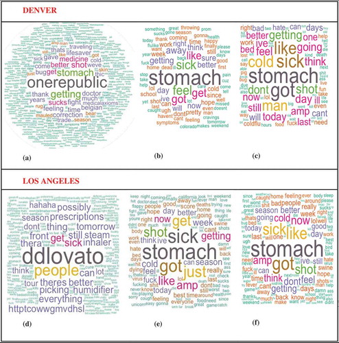
This study adopted a noise filtering procedure by removing RTs and tweets containing URLs. After filtering the non-geotagged tweets (Figure 1(c,f)), the highest frequency of words in the word cloud images is more lined up with the images of geotagged tweets as shown in Figure 1(b,e).

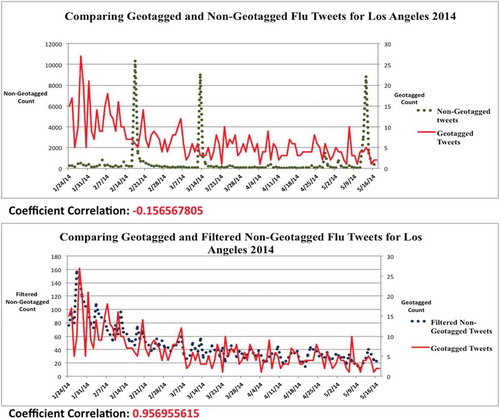
After looking at the word cloud images of flu tweets, the next step was to conduct the temporal trend analysis of geotagged, non-geotagged and filtered non-geotagged tweets. Figure 2 represents the daily trends and the correlation coefficient of tweeting frequencies in Los Angeles. Three peaks were observed in the non-geotagged tweets graph in Los Angeles (Figure 2). One user name by ‘ddlovato’ triggered these peaks. The first peak on 17 February showed the highest non-geotagged tweets count (10,300 RTs). It primarily focused on re-tweeting the message ‘RT @ddlovato: Doing everything I possibly can to get better by tomorrow. Humidifier, Thera Flu and steam inhaler!!! http://t.co/4wwgmvDhSL’. The second and the third peak of 13 March (9018 RTs) and 13 May (8,799 RTs) were largely produced by the messages ‘RT @ddlovato: I think this is why a lot of people don’t tour during flu season. Hahaha’, ‘RT @ddlovato: I’m sick so I’m picking up my prescriptions at 11 pm and there’s 7 people in front of me doing the same thing’.

Figure 2. The line charts indicating the daily trend analysis of the ‘flu’ tweets, including their weekly coefficient correlation for Los Angeles.

Similarly, the correlation coefficient in the Denver area among the flu tweets that is based on geotagged tweets and filtered non-geotagged tweets was much higher (0.474) compared to the coefficient correlation of geotagged tweets and non-geotagged tweets (0.029). The low correlation coefficient for the non-geotagged tweets is affected by the increase in the number of RTs (2 March 2014). Re-tweeting the messages of the user ‘Onerepublic’ mainly produced the peak of 2 March 2014. Some examples of these RTs were identified in order to understand the context of tweets in Denver: ‘RT @OneRepublic: Thank u to the Belgian doctor that gave us medicine to fight this flu – u r a lifesaver’, ‘RT @OneRepublic: Correction. Stomach flu sucks’, ‘RT @OneRepublic: Feeling much better. 2nd time we’ve come down with the 24 hr flu bug in 7 years’.

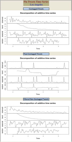
Time series analysis was used to reveal hidden patterns and to make sure if the correlation coefficient was accurate or not, since the Pearson correlation ignores the time factor. Figure 3 corresponds to the flu tweets time series in Los Angeles. The x-axis indicates the monthly time series (2 as February, 3 as March, 4 as April and 5 as May). The y-axis was split into four components. The observed component is based on the actual trend. The trend component was estimated by applying a smoothing procedure that calculated the moving average of each point. The seasonal component was estimated by calculating the average of the de-trended series (subtracting the trends estimate from the series). The random component was calculated by subtracting the trend and the seasonal component of the series. The random component was not utilized in this analysis. Figure 3 illustrates that the geotagged and the filtered non-geotagged tweets in Los Angeles followed the same pattern with a general decreasing trend from January to May; yet, the non-geotagged tweets did not follow the general pattern because of the noise created by the high percentage of RT. Figure 3 also shows that geotagged, non-geotagged and filtered non-geotagged tweets all revealed a seasonal (monthly pattern). Comparable to Los Angeles, the trend of geotagged and the filtered non-geotagged tweets (decreasing over time) in Denver was consistent.

Figure 3. The line charts consist of a trend component, seasonal component and an irregular or random component for flu tweets in Los Angeles.

In addition to decomposing the temporal trends to different components, it is important to look at the correlation between the geotagged and non-geotagged tweets in comparison to geotagged and filtered non-geotagged tweets based on the time factor.

The autocorrelation determines the linear dependency of a variable with itself at two points in time. In Denver and Los Angeles, there were significant autocorrelations of geotagged and filtered non-geotagged tweets, but there were no significant autocorrelations for non-geotagged tweets. When combining the geotagged and filtered non-geotagged tweets, significant autocorrelations were found; yet, no autocorrelation was detected when combining the geotagged and the non-geotagged tweets. The autocorrelation analysis results strongly reflect to the trend analysis in Figure 2.

Next, the Johansen procedure tests the long relationship (cointegration) between two or more variables. The variable (r) represents the number of cointegrated equation where (r = 0) means that there is no cointegration between the two variables. For instance, the test value in Los Angeles of the geotagged versus non-geotagged when r = 0 is 61.74. If the test (r = 0) greater than the critical value for say 5% (17.95), the null hypothesis is rejected and the alternative hypothesis is accepted. If the test (r ≤ 1) (20.94) is smaller than the critical value (8.18), the alternative hypothesis is accepted. In this case, there is no cointegration between the geotagged and non-geotagged tweets in Los Angeles. On the other side, there is a cointegration between geotagged and filtered non-geotagged tweets in Los Angeles, as the test (r = 0) (71.90) is bigger than the critical values, and (r ≤ 1) (5.54) is smaller than the critical values. In general, there are cointegrations between geotagged and filtered non-geotagged flu tweets within the Los Angeles, San Diego and New York, but there is no cointegration between the geotagged and non-geotagged flu tweets.

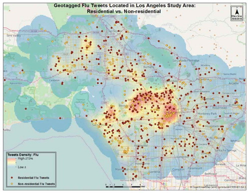
Figure 4 illustrates the spatial distribution patterns of geotagged tweets for the flu topic. The red areas indicate the hot spots where the flu tweet rates were highest in Los Angeles. This figure illustrates that the hot spots were found in the downtown and surrounding areas for Los Angeles. It also confirms that most geotagged ‘flu’ messages were tweeted from residential areas. For Denver, a similar spatial pattern emerged, yet the rate of tweets in Denver was much lower.

After overlaying the land-use layer, which was downloaded from the USGS over the geotagged flu layer in each city and after employing the ‘Spatial Join’ tool in ArcGIS, Table 3 shows that the residential areas collected the highest percentage compared to other land-use categories. A percentage of 48.81 of the geotagged tweets were located in residential areas. The spatial distribution of tweets for the ‘flu’ keyword was concentrated in residential areas, suggesting that most people tweet from home as they get sick.

Table 3. The spatial distribution of flu tweets based on land-use for the four study sites.

Land-use categories	Denver	Los Angeles	New York	San Diego	Percentage of land-usedistribution (%)
Bays and estuaries	0	1	1	3	0.21
Beaches	0	1	0	4	0.21
Commercial and services	40	216	219	88	23.13
Cropland and pasture	35	8	0	5	1.97
Evergreen forest land	0	0	0	1	0.04
Forested wetland	0	0	3	0	0.12
Herbaceous Rangeland	26	3	0	2	1.27
Industrial	1	22	17	2	1.73
Industrial and commercial complexes	0	0	9	0	0.37
Mixed rangeland	0	1	0	3	0.16
Mixed urban or built-up land	3	23	205	0	9.49
Non-forested wetland	0	1	1	0	0.08
Null area – no land-use assigned	0	0	1	0	0.04
Orchards, groves, vineyards, nurseries	0	1	0	3	0.16
Other agricultural land	0	2	0	0	0.08
Other urban or built-up land	3	21	14	7	1.85
Reservoirs	0	0	0	0	0.00
Residential	43	403	654	88	48.81
Shrub-brushland rangeland	0	11	0	32	1.77
Streams and canals	0	0	5	0	0.21
Strip mines, quarries and gravel pits	0	0	0	3	0.12
Transitional areas	3	7	5	14	1.19
Transportation, communication and services	4	21	140	5	6.98
Sum	158	742	1274	260	100.00

This table indicates the spatial distribution of flu tweets in each land-use category for Denver, Los Angeles, New York and San Diego and the percentage of land-use distribution for all cities combined. The rows highlighted in grey indicate the highest number of tweets that fall within the land-use distribution.

This table indicates the spatial distribution of flu tweets in each land-use category for Denver, Los Angeles, New York and San Diego and the percentage of land-use distribution for all cities combined. The rows highlighted in grey indicate the highest number of tweets that fall within the land-use distribution.

Figure 4. Kernel density map representing the hot spots of ‘flu’ tweets in relation to residential land-use areas in Los Angeles. The red colour indicating the highest density of tweets in the area, meanwhile the blue colour indicating the lowest density of tweets. The red points representing the Flu tweets that overlap with residential boundaries while the yellow points illustrate the Flu tweets that fall outside this boundaries ​ (a colour image is available in the electronic version) .​​​​​​

5.2. Comparison between geotagged and non-geotagged ‘Ted’ tweets

The word cloud images of non-geotagged Ted tweets were quite different from those for non-geotagged flu tweets. The word cloud analysis revealed that geotagged and non-geotagged Ted movie tweets were more consistent and shared similar contents in Denver and Los Angeles. The reason behind the consistency between word cloud images may be that the non-geotagged tweets for the ‘Ted’ keyword had less noise, and the RTs were more centred around watching the movie. This study adopted the noise-filtering procedure by removing RTs and tweets containing URLs. The word cloud images after the filtering process didn’t change much in term of highlighting the highest frequency of words using in tweets for the cities of Denver and Los Angeles.

After analysing the word cloud images of Ted tweets, the next step was to conduct the temporal trend analysis of geotagged, non-geotagged and filtered non-geotagged tweets.

Unlike the daily flu trends and their correlation coefficients, the daily trend analysis for ‘Ted’ in Figure 5 illustrates a stronger correlation between the geotagged tweets (shown in red) and non-geotagged tweets (shown in green). For instance, the coefficient correlation among the geotagged and non-geotagged tweets for the ‘Ted’ keyword in Los Angeles (0.926) was much higher than the one of flu tweets (−0.157) (Figure 2). However, after filtering the non-geotagged tweets (shown in blue) of the ‘Ted’ keyword, the coefficient correlation in Los Angeles (0.960) was still slightly higher compared to the correlation coefficient for the geotagged and non-geotagged tweets (0.926) (Figure 5). The higher correlation coefficient for the non-geotagged tweets was likely affected by the low number of RTs of the ‘Ted’ keyword.

Figure 5. The line charts indicating the daily trend analysis of the Ted tweets, including their weekly coefficient correlation for Los Angeles. All graphs have similar high peak on 29 June 2012.

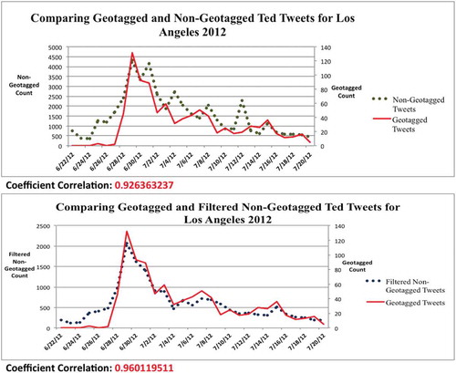
Thus, the filtering process improved the reliability of the non-geotagged tweets, but not in as pronounced a way as with the ‘flu’ keyword. Examples of geotagged and​​​​​​ non-geotagged tweet consistency among ‘Ted’ keyword in Denver and Los Angeles may be seen in such tweet messages as ‘Ted was so epic!!!:) great movie! Lol’, ‘Watching Ted, pretty excited’. The date of the high peak for geotagged and non-geotagged tweets was the same (29 June 2012). This date indicated the actual release date of the movie Ted.

Time series analysis was used to reveal hidden patterns and to determine if the correlation coefficient was accurate or not, given the inability of Pearson correlations to account for time or sequence. Geotagged, non-geotagged and filtered non-geotagged tweets among the keyword ‘Ted’ were consistent over time and the filtering process did not appear to affect the general trend substantially; in both the trend revealed exponential increases during the second week, specifically on the release date of the movie, and rapid decreases afterward. The x-axis for the ‘Ted’ keyword indicated a weekly time series (week 1 as from June 22 to June 28, week 2 as from June 29 to July 6, week 3 as from July 7 to July 13, week 4 as from July 14 to July 20).

In addition to decomposing the temporal trends for different components, the correlation between the geotagged and non-geotagged tweets was examined in comparison to geotagged and filtered non-geotagged tweets based on the time factor. The autocorrelation determines the linear dependency of a variable with itself at two points in time. Regarding the autocorrelations for the ‘Ted’ keyword in the cities of Denver and Los Angeles, there were no significant autocorrelations among the different elements in the charts (geotagged vs. no geotagged) and (geotagged vs. filtered non-geotagged). The reason behind this appears to be that the Ted tweets enfold one short cycle (1 day increase during the release date) in comparison to flu tweets that encompass a more distinct chronological pattern (several days).

Next, the Johansen procedure tests the long relationship (cointegration) between two or more variables. In this case, there was cointegration between geotagged vs. non-geotagged, and geotagged vs. filtered no geotagged Ted tweets in both cities of Los Angeles and San Diego, which indicates that variables have a long association or equilibrium relationship between them.

However, for Denver and New York, only the filtered non-geotagged tweets showed a sign of cointegration with the geotagged tweets, as the test value of (r = 0) (17.33, 17.96) was greater than the critical values of 15.66 and the test value of (r ≤ 1) (1.87, 7.63) was smaller than the critical values of 6.50. In brief, the filtered non-geotagged Ted tweets were still slightly correlated than non-geotagged tweets. This means that the trend analysis and the Pearson correlations were validated using the time series analysis in general, and Johansen test in particular.

Figure 6 illustrates the spatial distribution patterns of geotagged tweets for the ‘Ted’ keyword and verifies that the spatio-temporal pattern of tweets differs from one keyword to another. The red areas indicate the hot spots where the Ted tweet rates were highest. The hot spots of tweets for the ‘flu’ keyword were concentrated in the residential areas; the geotagged tweets in ‘Ted’ were focused in commercial and service areas of Denver and Los Angeles. The size of points in Figure 6 is related to the number of messages that were tweeted from the same location; the bigger the point is, the higher the number of tweets in that location. After zooming into the map of Los Angeles, the analyses established a high correlation between movie theatres and ‘Ted’ messages when people were tweeting from a shopping centre or a movie theatre.

Figure 6. Kernel density map representing the hot spots and the points of interest of Ted tweets in relation to commercial land-use areas in Los Angeles. The red colour indicates the highest density of tweets in the area, while the blue colour indicates the lowest density of tweets. The red circles represent the weighted point data of Ted tweets including the citation of points of interest in the highest weighted areas.

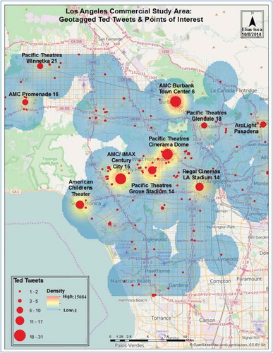
Table 4 adds the statistical perspective as a factor to assure that the number of ‘Ted’ tweets was focused in commercial and service areas when compared to other types of land-use. The highest percentage of geotagged tweets (33.03%) in all cities was concentrated in commercial and service areas. The only exception was New York where most of the geotagged tweets were concentrated in the residential areas (383 tweets) instead of commercial and service areas (277 tweets). The reason behind the different spatial distribution of geotagged Ted tweets may be related to the vertical structure of New York City and the mixed urban or built-up land. In order to accommodate a higher population density, the tall buildings and skyscrapers of New York City may blend a combination of different land-use types such as residential, commercial and industrial. This may be the reason why New York contained one of the highest numbers of geotagged tweets in the mixed urban and built-up land (286 tweets) in comparison to other cities such as Denver (3 tweets), Los Angeles (9 tweets) and San Diego (0 tweets).

Table 4. The spatial distribution of Ted tweets based on land-use for the four study sites.

Land-use categories	Denver	Los Angeles	New York	San Diego	Percentage of land-usedistribution (%)
Bays and estuaries	0	0	1	2	0.12
Beaches	0	1	1	0	0.08
Commercial and Services​​​​​​	65	409	277	90	33.03
Cropland and pasture	38	6	0	19	2.47
Evergreen forest land	0	0	0	13	0.51
Forested wetland	0	0	4	0	0.16
Herbaceous Rangeland	29	0	0	1	1.18
Industrial	1	64	53	3	4.75
Industrial and commercial complexes	0	2	32	0	1.34
Mixed rangeland	0	1	0	11	0.47
Mixed urban or built-up land	3	9	286	0	11.70
Non-forested wetland	0	0	11	2	0.51
Null area – no land-use assigned	0	0	1	0	0.04
Orchards, groves, vineyards, nurseries	2	0	0	0	0.08
Other urban or built-up land	8	26	15	20	2.71
Reservoirs	0	1	0	0	0.04
Residential	31	285	383	66	30.05
Shrub-brushland rangeland	0	15	0	34	1.92
Streams and canals	0	0	23	0	0.90
Strip mines, quarries and gravel pits	0	0	1	6	0.27
Transitional areas	3	1	21	9	1.34
Transportation, communication and services	12	48	91	10	6.32
Sum	192	868	1200	286	100.00

This table represents the spatial distribution of Ted tweets in each land-use category for Denver, Los Angeles, New York and San Diego and the percentage of land-use distribution for all cities combined. The rows highlighted in grey indicate the highest number of tweets that fall within the land-use distribution.

6. Principal findings

After conducting a series of data analysis tasks between geotagged tweets and non-geotagged tweets for two very distinct topic domains, this study suggests that the temporal trends of geotagged tweets have higher connection to topic choices than non-geotagged tweets (un-filtered) for some cases, and especially for the flu. This study reveals that non-geotagged tweets, if filtered appropriately, can also be a good source to monitor tweet data, especially for flu tweets. When removing the RTs and the URLs from the content of the non-geotagged tweet messages, the reliability coefficient correlation was significant in relation to geotagged tweets (Figure 2). This is caused by the abundance of RTs in the non-geotagged tweets. This abundance was influenced by realspace celebrities such as ‘Onerepublic’ in Denver and ‘ddlavato’ in Los Angeles. ‘One Republic’ is a popular rock band in Colorado and ‘Demi Lavato’ is a famous singer, songwriter and actress in the Los Angeles area. These patterns were not the case for the movie Ted tweets. The correlation coefficient of the filtered non-geotagged tweets for the movie Ted was slightly higher than the non-geotagged tweets in relation to the geotagged tweets (Figure 5). The results reveal how important the topic choice in Twitter is in shaping analysis and results. Based on the content analysis of the ‘flu’ keyword in Figure 1, the geotagged tweets of Denver and Los Angeles performed better than the non-geotagged tweets. The apparent underlying reason is that non-geotagged tweets may contain some data noise and the sharing information created by others, which can affect the content and the correlation of the tweets (Figure 2). Though the content analysis of the ‘Ted’ keyword demonstrates the absence of the data noise in the non-geotagged tweets, it demonstrates that both the geotagged tweets and the non-geotagged tweets can be informative and related to the topic. Correspondingly, the time series analysis (Figure 3) including the autocorrelation and Johansen test emphasizes similar results, indicating that filtered non-geotagged tweets perform better than non-geotagged tweets in tracking real-time events.

This study additionally discovered that high number of users tweeted about movie Ted from shopping centres and movie theatres. The apparent reason is that such users most likely had to use a phone, which usually contains a geotagged device; Table 4 and the map in Figure 6 illustrate this finding. Table 4 clarifies that the commercial category has the highest share of the movie ‘Ted’ tweets in all cities except New York. Due to the tall buildings and skyscrapers, the remote-sensing techniques in New York City may have failed to detect the accurate boundary of the land-use. Additionally, the vertical structure of New York was important in determining the spatial distribution of the geotagged tweets, where the mixed urban or built-up land type shared an excessive number of geotagged tweets for ‘Ted’ keyword (286 tweets) besides residential areas (383 tweets), and commercial and service areas (277 tweets). In contrast, Table 3 (‘flu’ keyword) and the map of Figure 4 show that residential areas dominated the ‘flu’ tweets. People tended to tweet from home when they got, or thought they were getting the flu, flu shot or stomach flu. As a result, the spatial relationship between tweets and land-use varies from one keyword to another.

7. Conclusion

The dynamic communication characteristics of Twitter data offer a great research opportunity for geographers to examine human activities and communications. Various theoretical efforts are underway to integrate cyberspace to realspace activity. For example, the M3D model (Spitzberg 2014) proposes that all social media, and most digital media, trade in memes, which are replicable forms for transmitting cultural information. Memes are hypothesized to diffuse more or less dependent upon five levels of influencing factors: the meme level (i.e. message factors), source (i.e. person), social network (e.g. density, span), societal (e.g. publicity, competing memes etc.) and geotechnical factors (i.e. smartphone adoption level). These factors and levels interact such that (a) real events sometimes elicit social media activity (e.g. Onerepublic, ddlevato getting the flu); (b) social media sometimes drive realspace activities (e.g. tweets promote others to see a movie); and (c) sometimes events elicit social media that evoke realspace activities, such as flu outbreaks provoking social media that influence people to get vaccinated. These three processes represent evememic, etymemic and polymemic episodes, and there is some evidence of all three in the tweet streams analysed here. Geotechnical processes (i.e. land-use), societal factors (e.g. movie campaigns), source (e.g. Demi Lovato) and meme (e.g. search term selection) all demonstrated some degree of complex interplay with the tweet streams, and what they were able to reveal about realspace events. This study utilized various quantitative, computational and GIS methods to investigate the content of geotagged tweets and non-geotagged tweets in two topics: public health (flu) and movie names (Ted). The analysis outcomes indicate a high dependency on the subject and topics of tweets when evaluating their contents and social network patterns. This study suggests that the use of filtered non-geotagged tweets is similar to the use of geotagged tweets when analysing their trends and patterns as they connect to realspace events. Using the data-filtering procedures applied in this study can reduce the percentage of noise in tweet data for some cases, and especially for analyses of flu-related tweets.

From an urban planning perspective, this study discovered that comparing geotagged tweets of multiple topics in social media (Twitter) can reveal significant spatial variation with the land-use distribution (such as residential land-use or commercial land-use). Additionally, the horizontal/vertical structure of cities may affect the spatial pattern of geotagged tweets. For instance, the vertical structure of New York City may have shifted most geotagged ‘Ted’ tweets to residential and mixed urban or built-up land areas instead of commercial and service areas. Tall buildings and skyscrapers may contain a combination of different type of land-use, which might hinder the real spatial distribution of geotagged tweets especially for the movie Ted case.

Limitations of this study include the bias of demography, missing data and the small percentage of geotagged tweets. The first limitation is the potential bias of demography from Twitter users. Many social media do not include detailed demographic information about users (Tsou 2015). Without knowing user profiles and their demography, the collection of tweets can be biased and unrepresentative of the wider Twitter population (Sloan and Morgan 2015). Twitter, in particular, is popular among young people, with almost 58% of its user base between the age of 16 and 34 (Tweedie 2014), whereas a much lower percentage of older adults use social media. Approximately 23% of online adults use Twitter to communicate online (Duggan 2015). For this reason, many data and opinions collected from social media may not be representative of the voices of the overall population. Besides, as of May 2016, Twitter is changing rules and in fact they are modifying the number of character in the text messages. These updates can have a significant impact on our methodology in collecting Twitter data.

Another constraint of this project is the missing data triggered by an error in the server system. The data collection server, which utilized GeoSearch APIs to collect tweets, failed to collect the flu tweets from 7 January to 23 January. Therefore, this study only uses the flu tweets from 23 January 2014 to 17 May 2014. The third constraint is the small percentage of geotagged tweets. The geotagged tweets consist of a small portion of the entire Twitter user population. Only 1–4% of tweets have GPS coordinates (Cheng, Caverlee, and Lee 2010; Tsou et al. 2013).

This research contributes to current or future research efforts in bridging GIS and social media analytics and draws a conclusive summary of how the spatio-temporal characteristics of Twitter data with geotagged and non-geotagged content are similar when filtered properly. Contribution of this study include (1) comparing geotagged and non-geotagged tweet messages based on different topic choices, (2) providing a framework to filter out the social media data noises from the tweet messages and (3) establishing a GIS method to determine the utilization of space within land-use based on geotagged Tweet messages. While performing a manual filtering process will allow filtering the noise from the non-geotagged tweets messages, however, this process is very time consuming and not practical for researcher attempting to study large datasets. A machine-learning approach supplemented with sentiment analysis algorithms is recommended in the future in order to produce better results. Further investigations are needed in this field to improve the accuracy of social media in predicting real-time events and allowing better surveillance methods in general and to detect disease outbreaks and market trends in particular.

Disclosure statement

No potential conflict of interest was reported by the author.​​​​​​

Additional information

Funding

This material is based upon work supported by the National Science Foundation: [Grant Number 1416509], IBSS project titled ‘Spatiotemporal ​​​​​​Modeling of Human Dynamics Across Social Media and Social Networks’ and National Science Foundation: [Grant Number 1634641], IMEE project titled ‘Integrated Stage-Based Evacuation with Social Perception Analysis and Dynamic Population Estimation’.

References

- Adams, P. C., S. Hoelscher, and K. E. Till. 2001. “Place in Context: Rethinking Humanist Geographies.” In Textures of Place: Exploring Humanistic Geography, edited by P. C. Adams, S. Hoelscher, and Till, xiii–xxxiii. Minneapolis: University of Minnesota Press.
- Akimoto, A. 2011. “Japan the Twitter Nation.” The Japan Times. http://www.japantimes.co.jp/life/2011/05/18/digital/japan-the-twitter-nation/.
- An, L., M. Tsou, S. Crook, J. M. Gawron, J. M. Gawron, and D. K. Gupta. 2015. “Space-Time Analysis: Concepts, Methods, and Future Directions.” Annals of Association of American Geographers 105: 891–914. doi:10.1080/00045608.2015.1064510.
- Aslam, A. A., M. H. Tsou, B. H. Spitzberg, A. Li, J. M. Gawron, D. K. Gupta, K. M. Peddecord, et al. 2014. “The Reliability of Tweets as a Supplementary Method of Seasonal Influenza Surveillance.” Journal of Medical Internet Research 16 (11): e250URL. doi:10.2196/jmir.3532.
- Barreneche, C. 2012b. “The Order of Places: Code, Ontology and Visibility in Locative Media.” Computational Culture http://computationalculture.net/article/order_of_places.
- Barreneche, C. 2012a. “Governing the Geocoded World: Environmentality and the Politics of Location Platforms.” Convergence 18 (3): 331–351.
- Boyd, D. M., and N. Ellison. 2007. “Social Network Sites: Definition, History, and Scholarship.” Computer Mediated Communication 13 (1): 1–11.
- Browning, B., and J. Sanderson. 2012. “The Positives and Negatives of Twitter: Exploring How Student-Athletes Use Twitter and Respond to Critical Tweets.” International Journal of Sport Communication 2012 (5): 503–521. doi:10.1123/ijsc.5.4.503.
- Chang, S., J. Sterne, W. Huang, H. Chuang, and D. Gunnell. 2010. “Association of Secular Trends in Unemployment with Suicide in Taiwan, 1959–2007: A Time-Series Analysis.” Public Health 124 (1): 49–54. doi:10.1016/j.puhe.2009.11.005.
- Cheng, Z., J. Caverlee, and K. Lee. 2010. “You are Where You Tweet: A Content-Based Approach to Geo-Locating Twitter Users.” In Proceedings of the 19th ACM International Conference on Information and Knowledge Management, edited by J. Huang, 759–768. New York: ACM.
- Chew, C., and G. Eysenbach. 2010. “Pandemics in the Age of Twitter: Content Analysis of Tweets during the 2009 H1N1 Outbreak.” PLoS One 5 (11): e14118. doi:10.1371/journal.pone.0014118.
- Chu, Z., S. Gianvecchio, H. Wang, and S. Jajodia. 2010. Who Is Tweeting on Twitter, Human, Bot, or Cyborg. Austin, TX: ACSAC.
- Cresswell, T. 2013. Geographic Thought: A Critical Introduction. Chichester: John Wiley & Sons.
- De Souza e Silva, A. 2013. “Location-Aware Mobile Technologies: Historical, Social and Spatial Approaches.” Mobile Media & Communication 1 (1): 116–121. doi:10.1177/2050157912459492.
- Downs, J. A., and M. W. Horner. 2012. “Probabilistic Potential Path Trees for Visualizing and Analyzing Vehicle Tracking Data.” Journal of Transport Geography 23: 72–80. doi:10.1016/j.jtrangeo.2012.03.017.
- Downs, J. A., M. W. Horner, G. Hyzer, D. Lamb, and R. Loraamm. 2014. “Voxel-Based Probabilistic Space-Time Prisms for Analyzing Animal Movements and Habitat Use. [Article].” International Journal of Geographical Information Science 28 (5): 875–890. doi:10.1080/13658816.2013.850170.
- Duggan, M. 2015. “Demographics of Key Social Networking Platforms |Pew Research Center.” http://www.pewinternet.org/2015/01/09/demographics-of-key-social-networking-platforms-2.
- Earle, P. 2011. “Twitter Earthquake Detection: Earthquake Monitoring in a Social World.” INGV, Istitut Nazionale Di Geofisica E Vulcanologia 54: 6. http://www.annalsofgeophysics.eu/index.php/annals/article/view/5364.
- Elwood, S. 2006. “Critical Issues in Participatory GIS: Deconstructions, Reconstructions, and New Research Directions.” Transactions in GIS 10 (5): 693–708. doi:10.1111/tgis.2006.10.issue-5.
- Esri. 2011. “ArcGIS Desktop.” http://help.arcgis.com/en/arcgisdesktop/10.0/help/index.html#//009z0000000s000000.htm.
- Esri. 2013. “ArcGIS Help 10.1.” http://resources.arcgis.com/en/help/main/10.1/index.html#//005p0000003s000000.
- Frias-Martinez, V. 2014. “Spectral Clustering for Sensing Urban Land Use Using Twitter Activity.” Engineering Applications of Artificial Intelligence. 35 237–245 doi:10.1016/j.engappai.2014.06.019.
- Guan, X. Y., and C. Chen. 2014. “Using Social Media Data to Understand and Assess Disasters.” Natural Hazards 74 (2): 837–850. doi:10.1007/s11069-014-1217-1.
- Hecht, B., L. Hong, B. Suh, and E. Chi. 2011. “Tweets from Justin Bieber’s Heart: The Dynamics of the Location Field in User Profiles.” In Proceedings of the 2011 Annual Conference on Human Factors in Computing Systems, edited by. D. Tan, 237–246. New York: ACM.
- Honeycutt, C., and S. C. Herring 2009. “Beyond Micro-Blogging: Conversation and Collaboration via Twitter.” In Proceedings of the 42nd Hawaii International Conference on System Sciences 1–10. Big Island: IEEE.
- Java, A., X. Song, T. Finin, and B. Tseng 2007. “Why We Twitter: Understanding Micro-Blogging Usage and Communities.” In Proceedings of the 13th ACM SIGKDD International Conference on Knowledge Discovery and Data Mining 56–65. New York: ACM.
- Johansen, S. 1995. Likelihood-Based Inference in Cointegrated Vector Autoregressive Models. Oxford: Oxford University Press.
- Kumar, S., F. Morstatter, and H. Liu. 2014. Twitter Data Analytics. New York: Springer.
- Luo, J., D. Joshi, J. Yu, and A. Gallagher. 2011. “Geotagging in Multimedia and Computer Vision—A Survey.” Multimedia Tools and Applications 51 (1): 187–211. doi:10.1007/s11042-010-0623-y.
- Nagel, A. C., M. H. Tsou, B. H. Spitzberg, A. Li, J. M. Gawron, D. K. Gupta, J. A. Yang, et al. 2013. “The Complex Relationship of Realspace Events and Messages in Cyberspace: Case Study of Influenza and Pertussis Using Tweets.” The Journal of Medical Internet Research 15 (10): e237. doi:10.2196/jmir.2705.
- Pawelek, K. A., A. Oeldorf-Hirsch, and L. B. Rong. 2014. “Modeling the Impact of Twitter on Influenza Epidemics.” Mathematical Biosciences and Engineering 11 (6): 1337–1356. doi:10.3934/mbe.
- Peterson, E. E., and J. M. V. Hoef. 2014. “STARS: An Arcgis Toolset Used to Calculate the Spatial Information Needed to Fit Spatial Statistical Models to Stream Network Data.” Journal of Statistical Software 56 (2): 1–17. doi:10.18637/jss.v056.i02.
- Reshef, D. N., Y. A. Reshef, H. K. Finucane, S. R. Grossman, G. Mcvean, P. J. Turnbaugh, … P. C. Sabeti. 2011. “Detecting Novel Associations in Large Data Sets.” Science 334 (6062): 1518–1524. doi:10.1126/science.1205438.
- Sakaki, T., M. Okazaki, and Y. Matsuo. 2013. “Tweet Analysis for Real-Time Event Detection and Earthquake Reporting System Development.” IEEE Transactions on Knowledge and Data Engineering 25 (4): 919–931. doi:10.1109/TKDE.2012.29.
- Sandoval-Almazan, R., and J. R. Gil-Garcia. 2014. “Towards Cyberactivism 2.0? Understanding the Use of Social Media and Other Information Technologies for Political Activism and Social Movements.” Government Information Quarterly 31 (3): 365–378. doi:10.1016/j.giq.2013.10.016.
- Sloan, L., and J. Morgan. 2015. “Who Tweets with Their Location? Understanding the Relationship between Demographic Characteristics and the Use of Geoservices and Geotagging on Twitter.” PLoS ONE 10 (11): e0142209. doi:10.1371/journal.pone.0142209.
- Spitzberg, B. H. 2014. “Toward A Model of Meme Diffusion (M 3 D).” Communicable Theoretical Communication Theory 24 (3): 311–339. doi:10.1111/comt.12042.
- Statista. 2017. “Twitter: Number of Monthly Active Users 2010–2017.” Statista. Accessed 30 June, 2017. http://www.statista.com/statistics/282087/numberof-monthly-active-twitter-users/.
- Ted. 2012. “Box Office Mojo.” http://www.boxofficemojo.com/movies/?id=ted.htm.
- Tsou, M. H. 2004. “Integrated Mobile GIS and Wireless Internet Map Servers for Environmental Monitoring and Management.” Cartography and Geographic Information Science 31 (3): 153–165. doi:10.1559/1523040042246052.
- Tsou, M. H. 2011. “Mapping Cyberspace: Tracking the Spread of Ideas on the Internet.” In Proceeding of the 25th International Cartographic Conference. Paris, France. http://icaci.org/files/documents/ICC_proceedings/ICC2011/Oral%20Presentations%20PDF/D3-Internet,%20web%20services%20and%20web%20mapping/CO-354.pdf
- Tsou, M. H. 2015. “Research Challenges and Opportunities in Mapping Social Media and Big Data.” Cartography and Geographic Information Science 42 (sup1): 70–74. doi:10.1080/15230406.2015.1059251.
- Tsou, M. H., J. Yang, D. Lusher, S. Han, B. Spitzberg, and J. M. Gawron. 2013. “Mapping Social Activities and Concepts with Social Media (Twitter) and Web Search Engines (Yahoo and Bing): A Case Study in 2012 US Presidential Election.” Cartography and Geographic Information Science 40 (4): 337–348. doi:10.1080/15230406.2013.799738.
- Tsou, M. H. and M. Leitner. 2013. “Visualization of Social Media: Seeing a Mirage or a Message?” Cartography and Geographic Information Science 40 (2): 55–60. doi:10.1080/15230406.2013.776754.
- Tweedie, S. 2014. “This Chart Reveals The Age Distribution At Every Major Social Network.” Business Insider. http://www.businessinsider.com/age-distribution-of-facebook-twitter-instagram-2014-11.
- USGS DS 240. 2014. “Enhanced Historical Land-Use and Land-Cover Data Sets: Download.” http://water.usgs.gov/GIS/dsdl/ds240/.
- Vieweg, S., A. L. Hughes, K. Starbird, and L. Palen. 2010. “Microblogging during Two Natural Hazards Events: What Twitter May Contribute to Situational Awareness.” In Proceedings of the SIGCHI Conference on Human Factors in Computing Systems, 1079–1088. CHI ’10. New York: ACM. doi:10.1145/1753326.1753486.
- West, S. G., and J. T. Hepworth. 1991. “Statistical Issues in the Study of Temporal Data: Daily Experiences.” Journal of Personality 59 (3): 609–662. doi:10.1111/j.1467-6494.1991.tb00261.x.
- Wilken, R. 2014. “Places Nearby: Facebook as a Location-Based Social Media Platform. [Article].” New Media & Society 16 (7): 1087–1103. doi:10.1177/1461444814543997.
- Yom-Tov, E., D. Borsa, I. J. Cox, and R. A. McKendry. 2014. “Detecting Disease Outbreaks in Mass Gatherings Using Internet Data. [Research Support, Non-U.S. Gov’t].” Journal of Medical Internet Research 16 (6): e154. doi:10.2196/jmir.3156.
- Yuan, M., and A. Nara 2015. “Space-Time Analytics of Tracks for the Understanding of Patterns of Life.” In Space-Time Integration in Geography and GIScience (pp. 373–398). Springer. http://link.springer.com/chapter/10.1007/978-94-017-9205-9_20.
- Zhao, B. 2015. “Detecting Location Spoofing in Social Media: Initial Investigations of an Emerging Issue.” Doctoral diss., Ohio State University.