Comparison of different spatial interpolation methods for historical hydrographic data of the lowermost Mississippi River

ABSTRACT

The lowermost Mississippi River (LMR) is important to the environment and economy of continental United States. Although bathymetric data have been collected over many decades at numerous cross-sectional sounding points, there has been no consensus on appropriate interpolator for generating bathymetry. Such interpolation is critical to reliable assessments of channel morphology and channel change, which serve for dredging, engineering projects, and mapping of navigation hazards. This study aimed to identify an optimal spatial interpolation for mapping the river bathymetry from cross-sectional sounding measurements. We evaluated a variety of spatial interpolation methods including Inverse Distance Weighting (IDW), Ordinary Kriging (OK), Radial Basis Function (RBF), and Local Polynomial Interpolation (LPI). In addition, we also considered the anisotropic form of IDW (Elliptical IDW as EIDW), that of OK (OKA), and Universal Kriging (UK). Two reaches in the LMR, located between approximately RM (River Miles) 170–140 and RM 60–35, were chosen as the study area. Those interpolators were compared in terms of root-mean-square error (RMSE), mean absolute error (MAE), bias, and coefficient of determination (r²). Our results demonstrate that both of RBF and OKA performed the best in mapping the bathymetry of study reaches. Furthermore, our results also indicate that the addition of anisotropy can significantly reduce RMSE by 5–20%, as compared to isotropic methods. The findings better inform other researchers on selecting a proper interpolation technique for mapping river bathymetry, particularly for other reaches of the Mississippi River.

KEYWORDS:

• Bathymetry
• spatial interpolation methods
• hydrographical cross-sections
• Mississippi River

1. Introduction

Fluvial topography (river bathymetry) plays an important role in detecting channel change, documenting sediment budgets and constructing numerical models for geomorphologic and ecological assessments (Crowder and Diplas 2000; Shen and Diplas 2008). The Mississippi River is one of the most important natural features in the continental United States, draining approximately 41% of land mass through its tributaries in the US. It has the seventh largest water discharge and suspended load among all world rivers (Milliman and Meade 1983; Meade 1996). In addition, the Mississippi River has been a backbone of commerce and industry, as its main channel provides a major transport corridor in the US. The lowermost Mississippi River (LMR) extends from the confluence of the Old River to the Gulf of Mexico (Figure 1), and serves as the busiest port area in the world (Gramling, Forsyth, and Wooddell 1998). A better understanding of riverbed bathymetry in LMR is critical to river navigation and environmental management, such as dredging and structural design (Conner and Tonina 2014). However, only a few studies had paid attention to constructing the river bathymetry of LMR reaches (Nittrouer, Allison, and Campanella 2008; Knox and Latrubesse 2016).

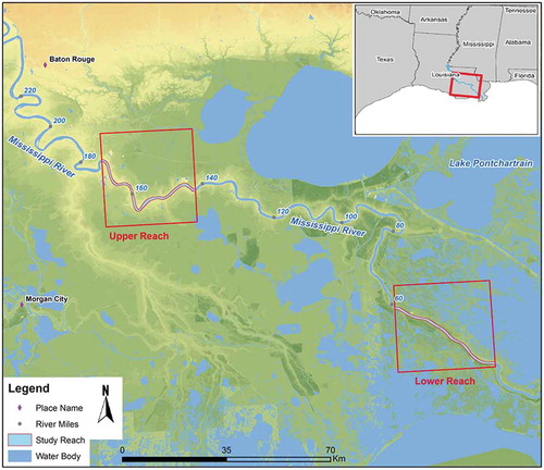
Figure 1. Map of the study area with two selected study reaches, namely the Upper Reach (UR) and Lower Reach (LR) in southeastern Louisiana; River Miles are also included in this map.

Spatial interpolation methods have been widely used to reconstruct bathymetric surfaces, but Different technologies, such as LIDAR (light detection and ranging), aerial photogrammetry and multi-beam sonar, have been greatly improved and applied to map the river bathymetry. Still, utilizing these techniques either cost expensively (such as multi-beam survey) or cannot detect the deeper parts (<2 m) of riverbed (such as LIDAR or aerial photogrammetry; Kinzel et al. 2007; Hilldale and Raff 2008). Field survey data have been and continue to be an efficient method to generate the accurate bathymetric maps (Brasington, Rumsby, and McVey 2000). A traditional approach for mapping river channels involves conducting a sequence of cross-sectional surveys along the river that gauge water depth information, typically a series of x, y, z coordinates along multiple transects. Many reach-scale studies rely on the cross-sectional surveys (e.g., Harmar et al. 2005; Yang, Townsend, and Daneshfar 2006; Legleiter and Kyriakidis 2008; Merwade 2009; Vetter et al. 2011; Conner and Tonina, 2014; Chowdhury et al. 2017), especially for the historical hydrographic surveys (e.g., Dury 1970; Sherwood et al. 1990; Hudson 2002). When historical hydrographic transects are collected in the same location repeatedly, these provide knowledge of how the river bathymetry varies through time.

Previous studies show that applying different interpolation methods could produce different results, even with the same input datasets (e.g., Declerq, 1996; Merwade, Maidment, and Goff 2006). More than 40 different spatial interpolation methods were classified, by Li and Heap (2008, 2011), into two major groups: deterministic and geostatistical methods. The deterministic techniques only apply mathematical functions for interpolation, which utilizes specified mathematical formulas to interpolate the surrounding measured values to determine the outcome values (Johnston et al. 2001). The interpolators such as TIN (Triangular Irregular Networks), IDW (Inverse Distance Weighted), RBF (Radial Basis Function) and LPI (Local Polynomial Interpolation), are classified as deterministic methods. On the other hand, the geostatistical methods rely upon both mathematical and stochastic models that consist of autocorrelation (statistical relationships between different measured points), which further allows the assessment of uncertainty in each outcome (Johnston et al. 2001; Chang 2006). Different forms of Kriging interpolators, such as Ordinary Kriging (OK), are typical geostatistical methods.

Several studies evaluated the interpolation methods for generating DEM (Digital Terrain Model) with different algorithms (e.g., Erdogan 2009; Boreggio, Bernard, and Gregoretti 2018; Chen et al. 2018a and b). For interpolating bathymetric data, in particular, past studies exhibited no consensus regarding which interpolation method performs the best in generating bathymetric surfaces. Several previous articles suggested that deterministic methods to be proper interpolators (e.g., Milne and Sear 1997; Sear and Milne 2000; Flanagin et al. 2007; Vetter et al. 2011; Panhalkar and Jarag, 2016; Amante and Eakins, 2016). Conversely, other studies proposed that geostatistical methods, especially OK, are appropriate interpolators to generate bathymetric topography not only in river channels (e.g., Carter and Shankar 1997; Legleiter and Kyriakidis 2008; Merwade 2009; Curtarelli et al. 2015), but also in other waterbodies, such as lakes or coastal regions (e.g., Bello–Pineda and Hernández–Stefanoni, 2007; Moskalik et al. 2013). Further, some other studies indicated that both geostatistical and deterministic methods have similar performance on creating bathymetric surface in their study area (e.g., Merwade, Maidment, and Goff 2006; Šiljeg, Lozić, and Šiljeg 2014; Chowdhury et al. 2017). In the entire Mississippi River and its tributaries, several studies have attempted to construct interpolated bathymetric maps with different interpolators (e.g., Pinter and Heine 2005; Flanagin et al. 2007; Little and Biedenharn 2014; Wang and Xu 2018). Table 1 summarizes all these studies in different environments. However, most of these studies only adopted a single interpolation method without comparing to other methods. Given the current debate on appropriate interpolation methods, it is a critical task to thoroughly compare the performance of various interpolation methods, particularly for the LMR.

Table 1. Summary of selected studies with corresponding interpolation methods in generating bathymetry. (A) summarizes the studies related to river channels (except Mississippi River); whereas (B) compiles the studies related to other waterbodies (i.e., coastal and lake). The studies in Mississippi River and its tributaries, especially LMR (Lowermost Mississippi River) are organized in (C).

Reference	Study area	Number of Methods compared ^1	Methods selected^2
(A) River Channel Studies
Carter and Shankar (1997)	Selwyn River and the North Ashburton River, New Zealand	1	OKA
Chowdhury et al. (2017)	Lower Athabasca River, Alberta, Canada	2	IDW, OK
Curtarelli et al. (2015)	Tucuruí hydroelectric reser, Brazil	4	OK
Legleiter and Kyriakidis (2008)	Merced River, California, USA	1	OK
Merwade (2009)	Six different river reaches, Texas and Kentucky, USA	7	OKA
Merwade, Maidment, and Goff (2006)	Brazos River, Texas, USA	7 or 8^3	EIDW, OKA
Milne and Sear (1997)/Sear and Milne (2000)	Seven river channels, upland Britain, UK	1	TIN
Panhalakr and Jarag (2016)	Panchganga River, India	3	IDW
Vetter et al. (2011)	Bregenzer Ache River, Austria	1	Natural neighbor
(B) Other Water Bodies
Amante and Eakins (2016)	Kachemak Bay, Alaska, USA	3	Spline
Bello–Pineda and Hernández–Stefanoni (2007)	Coast of Yucatan Peninsula, Mexico	2	OKA
Moskalik et al. (2013)	Hornsund Fjord, coast of Spitsbergen. Norway	12	OK
Šiljeg, Lozić, and Šiljeg (2014)	Lake Vrana, Croatia	14	RBF (multi-quadric), OK
(C) Mississippi River and Tributaries/Distributary studies
Flanagin et al. (2007)	Atchafalaya River and part of LMR	2	Spline (Kochanek-Bartels)
Little and Biedenharn (2014)	Entire LMR	1	TIN
Pinter and Heine (2005)	Lower Missouri River	1	TIN
Wang and Xu (2018)	Mississippi-Atchafalaya River diversion channel	1	IDW

1. The method compared number equals to 1 indicate the study merely apply one certain interpolator without further comparison.

2. Abbreviations for different interpolation: OK = Ordinary kriging, OKA = Ordinary kriging with anisotropy, IDW = Inverse distance weighting, EIDW = Elliptical inverse distance weighting, RBF = Radial basis function, TIN = Triangular irregular networks.

3. Merwade (2006) evaluated seven interpolation methods in Cartesian (x, y) coordinate, and eight methods in channel-centred (s, n) coordinate system.

2. Study data

From 1877 to the present, the US Army Corps of Engineers (USACE) has conducted hydrographic surveys for every decade along the Mississippi River (Little and Biedenharn 2014). These cross-sectional surveys provide a highly accurate and precise channel bathymetry to study historic channel morphology, river sediment budget or riffle-pool sequences (Hudson 2002; Harmar and Clifford 2007; Nittrouer et al. 2012; Knox and Latrubesse; 2016). The historic data has discrete sample points at cross sections and thus only constitutes a 1D (one-dimensional) representation. In order to generate continuous bathymetric surfaces (2D or 3D bathymetric models), these observed points should be interpolated by employing a proper spatial interpolation method.

This study uses a hydrographic survey conducted by USACE from April 1974 to November 1975 in the LMR. These datasets consist of the soundings (elevation measurements) that were taken perpendicular to the local downstream channel orientation. There were over 20 sounding vertices in each cross-section, with a lateral spacing around 30–50 m (Harmar et al. 2005; Harmar and Clifford 2007; Nittrouer et al. 2012). All channel depth soundings were processed and vertically referenced to NGVD 1929 (National Geodetic Vertical Datum of 1929). The original dataset covers the channel from Cairo at River Miles above the outlet (RM) 950 to the Head of Passes (RM 0) with 4515 cross-sections in total (Harmar and Clifford 2007).

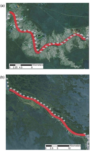
In order to examine whether an interpolation method is consistently optimal throughout the whole river channel, we extracted two reaches with different channel patterns, namely Upper Reach (UR) and Lower Reach (LR). The UR region is a meander dominant area, located between RM170 to RM140 (273–225 km upstream from Head of Passes; Figure 2(a)). There were 176 cross-sections with 6783 sounding measurements in the UR region. The other site (LR), from RM60 to RM35 (96–56 km upstream from Head of Passes; Figure 2(b)), has a lower sinuosity and straight channel pattern. The change in channel sinuosity could be attributed to downstream fining manifest in the increased clay content in bank and bed sediments (Fisk 1944; Mossa 1996). There were 144 cross-sections with 5739 sounding measurements in the LR region.

Figure 2. The bathymetric cross-sections in UR (a) and LR (b) reaches (see Figure 1 for the locations). Each cross-section contains ~20 to 30 soundings labelled in red dots. The numbers represent River Miles. Note that although the original hydrographic surveys were labelled in English unit (mile, feet), all the calculated results are converted into metric system.

3. Methods

This study aimed to compare the performance of various spatial interpolation methods in the LMR to assist further channel change and engineering studies. Three steps were involved in the study design, including: (1) a transformation of cross-sectional soundings to a channel-centred (s, n) coordinate system, (2) applications of different interpolators to generate bathymetric maps, (3) assessment of interpolation methods based on statistical criteria. Details of each step are described in below.

3.1. Converting data into channel-centred (s, n) coordinate system

With meandering, sinuosity and flow direction change, the characteristics of river channel topography often bring the challenges in analysing river channel data. For example, most GIS packages of interpolation tools only fit the Cartesian coordinates (x, y), which presumes a straight line distance between a pair of two points by a straight line. However, the true distance between this pair of points should be calculated along the river channel. Therefore, transforming the original data from a Cartesian system (x, y) into a channel-centred spatial referencing system (s, n) is a necessary procedure of data pre-processing (e.g., Parker and Ikeda 1989; Deutsch and Wang 1996; Goff and Nordfjord 2004; Legleiter and Kyriakidis 2006, 2008; Merwade, Maidment, and Goff 2006; Merwade, Cook, and Coonrod 2008; Merwade 2009; Trevisani, Cavalli, and Marchi 2010).

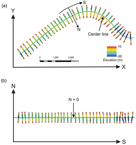
The channel-centred coordinate system (s, n) is defined by both the s-axis (along the flow direction) and n-axis (across the flow direction, and perpendicular to s-axis) (Merwade, Maidment, and Hodges 2005). Several previous studies introduced how to assign channel-centred (s, n) coordinates to the cross-sectional points by using either GIS procedures or mathematical algorithms (Merwade, Maidment, and Hodges 2005; Legleiter and Kyriakidis 2006, 2008). These techniques involve ‘straightening’ procedures to transform the point measurements from regular Cartesian (x, y) system (Figure 3(a)) into a channel-centred (s, n) coordinate system (Figure 3(b)). We adopted the transformation method designed by Merwade, Maidment, and Hodges (2005). The first step was to map the channel centreline as a reference. Second, points were assigned (s, n) coordinates, where s was the distance along the channel centreline with upstream end of the river as its origin (s= 0) and n was distance across the centreline (or s-axis) of the flow direction (as the centreline in Figure 3(a)). Looking downstream along the n-axis, all n coordinates were positive on the right hand side of s-axis, and vice versa. Lastly, plotting the cross-section vertices data in the new channel-centred (s, n) coordinate (Figure 3(b)). The channel geometry is straightened by using (s, n) coordinates, and then the sounding data can be treated with respect to the flow direction.

Figure 3. An example of coordinate transformation from Cartesian (x, y) coordinate system (a) into channel-centred (s, n) coordinate system from a selected portion in study reaches. The channel centreline is shown in (a), which would be transformed to reference line with n = 0 in n-axis in (b). The soundings with different colour represent the bed elevation.

3.2. Interpolation methods

Different interpolation methods were compared in our study. Among them, all the interpolators are all deterministic methods, except the Kriging family, such as OK and UK (Universal Kriging). Both of them are geostatistical methods. All analysis were accomplished by using the Geostatistical Analyst extension in ArcGIS 10.3.

3.2.1. Inverse distance weighted (IDW) and elliptical inverse distance weighting (EIDW)

IDW is based on the assumption that the sampled points closer to the predicted points have more influence on predicted value than the sample points farther apart. Thus, IDW predicts the estimated value by averaging over all the known measurements, and assigning greater weight to nearer points (Shepard 1968; Philip and Watson 1982). The IDW is formulated as follows:

(1) $Z\left(x\right)=\frac{\sum _{i=1}^n{W}_i{Z}_i}{\sum {}_{i=1}^n{W}_i}$(1)

(2) $W_i=\frac{1}{d_i^k}$(2)

where $Z\left(x\right)$ is the estimated value at a predicted point, and $Z_i$ is the observed value at point $i$. $W_i$ is the weight value assigned at point $i$, and$d_i$ is the distance between point $i$ and the predicted point; moreover, k is the power variable. The power variable decides how surrounding points affect the estimated value. A lower power results in higher influence from distant points.

The regular IDW method assumes an isotropic surface and thus uses a circle as the search neighbourhood (Figure 4). A modified version known as EIDW (Elliptical Inverse Distance Weighting), proposed by Tomczak (1998) and Merwade, Maidment, and Goff (2006), further considered anisotropy by assigning greater weight to the direction with greater influence. The EIDW method utilizes an elliptical search neighbourhood (Figure 4) that contains more points lying along the flow direction. Thus, in our case, the sounding point alignment along the river flow direction would have greater predictive control than the sounding point alignment transverse to the river flow. In other words, at the same distance, a sounding point would receive greater weight by using the EIDW method if measured along the river flow direction. It is critical to define the anisotropy ratio ($a_r$) in EIDW method, defined as:

(3) $a_r=\frac{a}{b}$(3)

Figure 4. IDW interpolation methods (a) with sampled points P1 to P5 and unsampled point P in the centre, circular with dashed line represent its search neighbourhood, note that P5 is excluded in the search circle. Nevertheless, (b) shows elliptical search neighbourhood for EIDW algorithm (major axis = a, minor axis = b), and P5 is included in this case. (Modified from Merwade, Maidment, and Goff 2006).

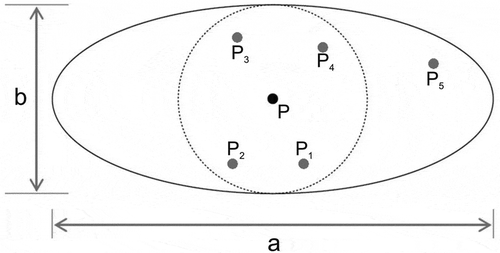
where a = major axis and b = minor axis of the elliptical search neighbourhood. In our study, both simple IDW and EIDW methods were evaluated.

3.2.2. Ordinary Kriging (OK) and Universal Kriging (UK)

Kriging is a type of geostatistical interpolation method with abundant variants, and OK is the fundamental method in the Kriging family. In general, the OK interpolator is based on an assumption of random spatial processes with stationarity, and aims to offer unbiased estimation with a minimized error variance (Isaaks and Srivastava, 1989; Cressie 1990; Carter and Shankar 1997; Goovaerts 1997). The basic formula for OK is expressed as:

(4) $Z\left(x\right)=\sum _{i=1}^n{W}_i{Z}_i$(4)

All the parameters have the same meanings as those in Equations (1) and (2). Nevertheless, unlike the IDW method, the weighting coefficient ($W_i$) in the OK system is assigned by not only considering the distance between unsampled and sampled points, but also the spatial correlation between these points. To ensure an unbiasedness results, the following condition must be maintained:

(5) $\sum _{i=1}^n{W}_i=1$(5)

In addition, the error variance (${\sigma }^2$) is expressed as:

(6) ${\sigma }^2=\frac{\sum _{i=1}^n{\left(Z\left(x\right)-Z_i\right)}^2}{n}$(6)

where n represents the total numbers of data points. To minimize the error variance, the derivatives of Equation (6) over each weight should equal zero, and thus can be written as a ($n+1)$ matrix system with the Lagrange parameter (μ) included in the matrix system:

(7) $\left[\begin{array}{ccccc}0& {\gamma }_{1,2}& \cdots & {\gamma }_{1,2}& 1\\ {\gamma }_{2,1}& 0& \cdots & {\gamma }_{2,n}& 1\\ ⋮& ⋮& ⋮& ⋮& 1\\ {\gamma }_{n,1}& {\gamma }_{n,2}& \cdots & 0& 1\\ 1& 1& \cdots & 1& 0\end{array}\right]\bullet \left[\begin{array}{c}{w}_1\\ w_2\\ ⋮\\ w_n\\ -\mu \end{array}\right]=\left[\begin{array}{c}{\gamma }_{1,x}\\ {\gamma }_{2,x}\\ ⋮\\ {\gamma }_{n,x}\\ 1\end{array}\right]$(7)

where $\gamma$ are the semivariogram values between the pairs of points $1ton$, and $x$ is the point where the unknown value is estimated from the known ($1\cdots n$). The key to Kriging’s flexibility is the semivariogram ($\gamma$), or simply variogram; which is described by a mathematical expression of:

(8) $\gamma \left(h\right)=\frac{1}{2N\left(h\right)}\sum _{i=1}^{N\left(h\right)}{\left[Z\left(x_i\right)-Z\left(x_i+h\right)\right]}^2$(8)

where $N\left(h\right)$is the number of sample pairs separated by a distance of h; $Z\left(x_i\right)$ and $Z\left(x_i+h\right)$ are sample values at a pair of data points separated by the distance (lag) of h. Taking$\gamma \left(h\right)$ with directional influences into account is often referred to anisotropic OK or OK with anisotropy (Eriksson and Siska 2000; Merwade, Maidment, and Goff 2006). In this study, we labelled this method as OKA. The OKA method calculates the Kriging weights by examining anisotropy direction in semivariogram map (Johnston et al. 2001). In our study, we utilized a two-dimensional (S and N) semivariogram model to calculate weights.

The other form of Kriging interpolation is the Universal Kriging (UK). The concept of UK method is based on the OK method, but assumes that a smoothly varying and non-stationary trend (or drift) adds to the random process component. The model is represented by the following formula:

(9) $Z\left(x\right)=\mu \left(x\right)+\epsilon \left(x\right)$(9)

where $\mu \left(x\right)$ is the trend function at location x, and $\epsilon \left(x\right)$ is the difference between the observed value and the trend value, or referred as random error. The problem of trend was first recognized by Matheron (1969), and been adopted in several different studies (e.g., Legleiter and Kyriakidis 2008; Kiš 2016). In our study, the trends from both S and N dimensions has also been taken into account for. Thus, OK, OKA and UK interpolators were all evaluated in our study.

3.2.3. Radial basis function (RBF)

The concept of RBFs is to fit a smooth surface through the measured sample values while minimizing the curvature of the surface (Aguilar et al. 2005; Xie et al. 2011; Chen et al. 2018a, 2018b). Talmi and Gilat (1977) first constructed the mathematical background of RBFs; as a rule, the variable Z in a prediction point x can be expressed as the sum of two components (Mitášová and Mitáš 1993):

(10) $Z\left(x\right)=T\left(x\right)+\sum _{j=1}^n{b}_j\psi \left(d_j\right)$(10)

where $\psi \left(d_j\right)$ is the radial basis functions, and $d_j$is the distance between sample point to prediction point $x$, and n being the number of sampling points. The ‘trend’ function,$T\left(x\right)$, is given by the following expression:

(11) $T\left(x\right)=\sum _{i=1}^m{a}_i{f}_i\left(x\right)$(11)

where $f_i\left(x\right)$is a set of linearly independent functions, or could be considered as a member of a basis for the space of polynomials of degree <m. Both coefficients $b_j$ and $a_i$ are obtained by solving the following n + m system of linear equations:

$Z\left(x_k\right)=\sum _{i=1}^m{a}_i{f}_i\left(x_k\right)+\sum _{j=1}^n{b}_j\psi \left(d_{jk}\right)\mathrm{f}\mathrm{o}\mathrm{r}k=1,2,\dots ,n$

(12) $\sum _{j=1}^n{b}_j{f}_k\left(x_j\right)=0\mathrm{f}\mathrm{o}\mathrm{r}k=1,2,\dots ,m$(12)

where n is the total number of sampling points used in in the interpolation of the surface $Z\left(x\right)$. In ArcGIS system, one could choose from five different RBF methods that fit $\psi \left(d\right)$ in Equation (12), namely as: completely regularized spline (CRS), multi-quadric function (MF), inverse multi-quadric function (IMF), thin-plate spline (TPS), and spline with tension (ST). The following formulas express these five different cases (Xie et al. 2011):

CRS:  $\psi \left(d\right)=ln{\left(\frac{\sigma d}{2}\right)}^2+E_1{\left(\sigma d\right)}^2+\gamma$

MF:  $\psi \left(d\right)=\sqrt{d^2+{\sigma }^2}$

IMF:  $\psi \left(d\right)=\frac{1}{\sqrt{d^2+{\sigma }^2}}$

TPS:  $\psi \left(d\right)={\sigma }^2{d}^{2}ln\left(cd\right)$

(13) $\mathrm{S}\mathrm{T}:\psi \left(d\right)=ln\left(\frac{\sigma d}{2}\right)+I_0\left(\sigma d\right)+\gamma$(13)

where σ is the optimal smoothing parameter, $d$ equals the distance from sample to prediction point, $I_0\left(\hspace{0.17em}\right)$ is the modified Bessel function; $E_1\left(\hspace{0.17em}\right)$ is the exponential integral function, and $\gamma$ is Euler’s constant. Each basis function has a different shape and results in a slightly different interpolation surface. Among them, the TPS algorithm performs the best in our analysis, and therefore was chosen in our study (more detail provided in the Results and Discussion).

3.2.4. Local polynomial interpolation (LPI)

LPI is a process of searching a (polynomial) formula, whose curve is fitted to a local subset of points. Unlike the global polynomial interpolation (GPI), which fits a polynomial to the entire dataset and captures coarse-scale pattern in the data, LPI compromises the moving average procedure with GPI methods. LPI is fitted to a local subset defined by a moving window. This window should include a reasonable number of data points; thus, the size of the window needs to be large enough for this process (Johnston et al. 2001; Xie et al. 2011).

3.3. Validation of interpolated surfaces

There are two common validation methods that have been widely suggested for evaluating of the accuracy of interpolation methods. The first method is a cross-validation method, namely as ‘leave-one-out technique’. This method involves omitting a single sample value from the entire dataset, and performing interpolation procedure by using the remaining dataset. After the interpolation process, the difference between the actual and predicted values of the omitted point is then calculated. This procedure is repeated for n times, where n equal to the number of all samples. The ‘leave-one-out’ cross-validation is embedded in the ArcGIS Geostatistical Analyst extension, which provide an exploratory analysis results.

The other validation method is called as ‘split-sample method’. In this method, the entire raw dataset is divided into two subsets: the training dataset and the test datasets. The training dataset is used to produce the interpolated surface, and the performance of each interpolation method is evaluated by comparing the difference between the predicted and observed values from the test dataset. In our study, the entire dataset was split into training datasets, which contain ~70% of all the points, and test datasets (~30% of the total points). In detail, 4748 points out of 6783 soundings were split into training dataset in UR region, and training dataset in LR region contained 4017 out of 5739 soundings. The ‘leave-one-out technique’ was performed by using the training dataset solely, and the ‘split-sample method’ was applied to calculate the differences in test dataset. Both of these methods could assess the stability of each interpolation algorithm (Declerq, 1996; Smith, Holland, and Longley 2005; Erdogan 2009).

Several statistical measurements are most widely used to evaluate the overall performance of interpolation methods, including of root-mean-square error (RMSE), mean absolute error (MAE), bias and coefficient of determination (r²).s (Isaaks and Srivastava, 1989; Zar 1999; Li and Heap 2008). The following mathematical equations show how to calculate these statistical measurements:

(14) $RMSE=\sqrt{\frac{1}{n}\sum _{i=1}^n{\left(Z_i-Z{\left(x\right)}_i\right)}^2}$(14)

(15) $MAE=\frac{1}{n}\sum _{i=1}^n\left|Z_i-Z{\left(x\right)}_i\right|$(15)

(16) $Bias=\frac{1}{n}\sum _{i=1}^n\left(Z_i-Z{\left(x\right)}_i\right)$(16)

(17) $r^2={\left[\frac{\sum _{i=1}^n\left(Z_i-\overline{Z_i}\right)\left(Z{\left(x\right)}_i-\bar{Z}{\left(x\right)}_i\right)}{\sqrt{\sum _{i=1}^n{\left(Z_i-\overline{Z_i}\right)}^2\sum _{i=1}^n{\left(Z{\left(x\right)}_i-\bar{Z}{\left(x\right)}_i\right)}^2}}\right]}^2$(17)

where n is the number of data points in the test dataset. Also, once again, $Z_i$ is the observed value at point i, and $Z{\left(x\right)}_i$ is the corresponding estimated value by using a specific interpolator at the same point. In Equation (14), $\overline{Z_i}$ and $\bar{Z}{\left(x\right)}_i$ represent the average values of the observed and estimated values, respectively.

In summary, seven different interpolators, including IDW, EIDW, OK, OKA, UK, TPS and LPI algorithms, were evaluated in this study. All the parameters from each interpolators (Table 2) were optimized by employing the statistical criteria. More details are introduced in the following paragraph.

Table 2. Parameters used in the different spatial interpolation methods in both of UR (A) and LR (B) regions.

Method	Parameters^1
(A) Upper River Reach
OK	Semi-axis length = 1792.5; lag size = 219; range = semivariogram model = stable
OKA	Major semi-axis length = 1020; minor semi-axis length = 2640; lag size = 220; semivariogram model = stable; anisotropy direction = 180
UK^2	Model 1: major semi-axis length = 4800; minor semi-axis length = 1602.5; lag size = 400; semivariogram model = exponential; anisotropy direction = 90 Model 2: major semi-axis length = 350; minor semi-axis length = 4800; lag size = 400; semivariogram model = stable; anisotropy direction = 180
IDW	Semi-axis length = 37,880.5; power = 4
EIDW	Major semi-axis length = 10,000; minor semi-axis length = 60,000; anisotropy factor = 0.166; power = 3
TPS (RBF)	Major semi-axis length = 10,000; minor semi-axis length = 50,000; anisotropy factor = 0.2
LPI	Semi-axis length = 989.2; polynomial order = 1; kernel function = exponential
(B) Lower River Reach
OK	Semi-axis length = 530; lag size = 70.3; semivariogram model = stable
OKA	Major semi-axis length = 3600; minor semi-axis length = 1276; lag size = 300; semivariogram model = stable; anisotropy direction = 90
UK	Major semi-axis length = 4500; minor semi-axis length = 800; lag size = 400; semivariogram model = exponential; anisotropy direction = 90
IDW	Length of semi-axis = 31,901.6; power = 4
EIDW	Major semi-axis length = 6000; minor semi-axis length = 66,000; anisotropy factor = 0.09; power = 4
TPS (RBF)	Major semi-axis length = 8000; minor semi-axis length = 60,000; anisotropy factor = 0.2
LPI	Semi-axis length = 1016.; polynomial order = 1; kernel function = exponential

1. The lag numbers = 12 for all Kriging-based interpolators.

2. The best parameters for UK algorithm in UR reach is the compromised models from Model 1 and 2.

4. Results and discussion

4.1. The optimized models selection

In order to select the parameter for the OK interpolation family, both anisotropy and trends in both UR and LR areas were computed and checked. Figure 5A and B illustrate the results of trend analysis from both UR and LR. The general patterns from both figures exhibit no significant trend in s-axis directions (X-axis, along flowlines), as the red lines are relatively straight. However, the trend lines in blue lines along y-axis demonstrate that n-axis directions (across channel) have a symbolic upside-down U shape in both UR and LR. The purpose of the trend analysis tool is to visualize any large-scale trends in our data that might need to be removed prior to estimation (Johnston et al., 2001). Our results suggest that our data points have a second-order trend in the n-axis direction, and this second-order trend might need to be removed for further analysis. Thus, we tested three different types of OK interpolators for our study: a simple OK, OKA with considering anisotropy and UK with not only considering anisotropy, but also removing the trend.

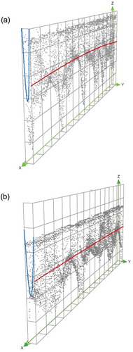
Figure 5. Trend analysis for the cross-sectional data in UR reach (A) and LR region (B) in 3D frames. Both figures were created by using ArcGIS. The green lines represent x, y, z dimensions. Each black dot symbolizes the bathymetric measurement; and -axis display vertical elevation. Note that in channel-centred (s, n) coordinates, red and blue lines represent the trend lines for x-direction (s-axis) and y-direction (n-axis), respectively.

The semivariograms in UR reach (Figure 6A) and LR reach (Figure 6B) were generated by considering 12 lags. The colourful circle inserted on top of each semivariogram is the “semivariogram map”, which is utilized to demonstrate the anisotropy direction. Clear anisotropy could be found on both semivariogram surfaces; with the azimuth of maximum continuity direct about 180 degree (indicated by red dashed line in Figure 6A) and 90 degree (Figure 6B). The strong anisotropy might suggest the direction of the cross-section’s influence on the spatial variability of the data. In addition, Figure 6A and B also display the average semivariance (symbols) and fitted models (solid lines) by employing the OKA parameters shown in Table 2. These parameter values were defined by considering the spatial autocorrelation (from semivariogram surfaces) and the criteria provided by Johnston et al. (2001). First, the mean errors for each model should be close to zero. Second, the RMSE values and average standard errors should be as small as possible. To guarantee the optimized models been selected, we constrained the value of mean error for each model between -0.5 and 0.5 m (Table 3A and B), which yielded the RMSE values for different models comparable.

Table 3. Summary of the statistical results for different interpolation methods by using leave-one-out cross-validation in UR (A) and LR (B) reaches.

	IDW	EIDW	OK	OKA	UK	TPS	LPI
(A)
RMSE (m)	3.00	2.35	2.18	1.90	1.84	1.86	3.04
MAE (m)	1.64	1.41	1.21	1.07	1.07	1.05	1.69
Bias (m)	−0.103	−0.010	−0.069	−0.015	0.034	0.028	0.314
r^2	0.94	0.96	0.97	0.98	0.98	0.98	0.94
(B)
RMSE (m)	3.28	2.37	2.53	2.11	2.11	2.06	3.22
MAE (m)	1.55	1.24	1.24	1.07	1.13	1.02	1.79
Bias (m)	−0.113	−0.011	−0.141	0.000	0.005	0.020	0.424
r^2	0.90	0.95	0.94	0.96	0.96	0.96	0.91

Figure 6. The experimental semivariograms and semivariogram maps (the ellipse with different colors) in UR (A) and LR (B) areas for consideration of OKA algorithm. Clear anisotropy could be found with main direction at degree of 180 (A) and 90 (B) labeled with red dashed lines. Both experimental semivariograms were created by considering anisotropy and the parameter in Table 2.

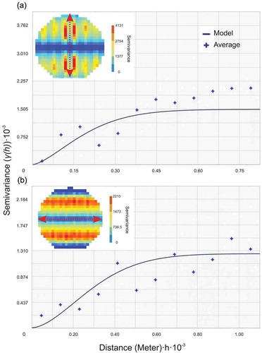
All these rules were applied on identifying the optimized interpolation models, especially for the interpolators with anisotropic considerations. For instance, the parameters adopted in Figure 6A and B yield the mean errors between 0 and -0.015 m; which ensures the validity of the spatial analysis and the accuracy of OKA models. This information facilitates the decision-making procedures by evaluating which interpolation algorithm provides the most accurate interpolated prediction. Similar norms were also applied to different interpolators; for example, the optimized anisotropy factors for EIDW interpolator are found to be 0.166 in UR region and 0.09 in LR region (Table 2). In addition, TPS algorithm has also been recognized with best performance among all the RBF algorithms (with the only RMSE value < 2 m) by applying these principles, and therefore chosen by our study.

4.2. Channel bathymetry generation

With all the optimized models with seven different interpolation algorithms been confirmed, the interpolated surfaces with these models are exhibited in Figure 7 (UR region) and 8 (LR region). Although these interpolation methods are consistent in describing the general topographic trends, significant differences can be discovered from the interpolated maps. The interpolated surfaces with OK, IDW and LPI methods demonstrate more abrupt topography; while all the other interpolation methods (UK, OK, EIDW and TPS algorithms) tend to generate a smoother, realistic bathymetric surfaces; both Figures 7 and 8 also show similar trends. Moreover, due to the second-order trends in the n-axis direction removed in UK algorithm, Figures 7(c) and 8(c) display a smooth surface, but fewer geographical features been displayed. In particular, the meander bends that can be found in all other interpolated maps, could not be perceived in both these surfaces.

Figure 7. The interpolated bathymetric surface in UR regions by using different interpolation methods of OK (a), OKA (b), UK(c), IDW (d), EIDW (e), TPS (f) and LPI (g). The square with black line indicates the location of Figure 9(a,c).

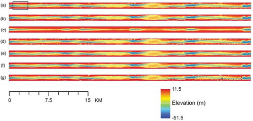
Figure 8. The interpolated bathymetric surface in LR region, with similar order of interpolation methods from Figure 7. The square with black line represents the location of Figure 9(b,d).

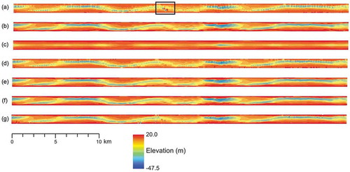
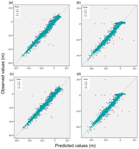
Figure 9. Different scatter-plots between observed and estimated elevation values by using interpolators of OK ((a) in UR region, (b) in LR region) and TPS ((c) in UR reach and (d) in LR reach). Different colour represent different rank ((a) to (d)) with absolute error range (A < 5 m, B = 5–10 m, C = 10–15 m, D > 15 m).

Generally, these interpolated surfaces indicate that OKA, EIDW and TPS interpolation methods might have better performances. However, the main purpose of this study is to assess the performances of different interpolators by using statistical criteria. Hence, the interpolated surfaces would be further assessing by integrating the following statistical results.

4.3. Results from leave-one-out technique

The cross-validation results from leave-one-out technique in UR region are shown in Table 3A. Among all the interpolation methods evaluated, OAK, UK and TPS interpolators lead the r² values of 0.98. Moreover, UK, OKA and TPS algorithms have the lowest RMSE results (≤1.90 m) and MAE values (≤1.07 m). Thus, by evaluating both RMSE and MAE results, it is obvious that these three algorithms share the best interpolators in this study reach. If one put the bias results into consideration, OKA algorithm performs better than TPS and UK algorithm. Also, unlike the bias results for both UK and TPS interpolators, the bias for OKA with negative value (bias = −0.015) demonstrates a slight tendency to underestimate the bathymetric depth.

On the other hand, both LPI and IDW interpolators have the worst performance among all the interpolation methods in UR area with highest RMSE (both ≥3 m) and MAE values (both >1.6 m). Additionally, when we accounted for anisotropic consideration and reformed IDW to EIDW, and OK to OKA or UK, the RMSE and MAE values decreased significantly. As Table 3A shows, the values of RMSE for EIDW, OKA and UK decrease around 20% compared to their original interpolator. Also, if taking the MAE values of the original interpolator as a reference, the new methods with anisotropic consideration decrease these values around 12% to 15%. Thus, the importance of anisotropic considerations is unfolded while interpolating the river bathymetric datasets.

In the LR region, the overall results show relatively similar pattern as well as the results from UR region (Table 3B), but with higher RSME and MAE values. TPS algorithm leads the performance on both RMSE and MAE results, following by both UK and OKA algorithms. Surprisingly, OAK algorithm has the best behaviour in bias value (bias = 0.00) with almost no bias on interpolating the training dataset, succeeding by UK algorithm. Conversely, with high RMSE and MAE results, as well as strong bias, LPI algorithm has the worse overall performance in LR, following by IDW algorithm (both RMSEs >3.2 m, MAEs >1.5 m). In addition, the importance of anisotropic considerations is observed again in the LR region (Table 3B). Similar to the results from UR reach (Table 3A), Table 3B also demonstrates that the RMSE and MAE values of interpolators with anisotropic consideration (EIDW, and OK to OKA or UK) significantly decrease. Comparing to their original form of OK and IDW algorithms, the reduction of RMSE results are about 17% to 28%; furthermore, MAE results also decline about 9% to 20%.

By scrutinizing the results from both UR and LR regions, it is recognizable that both LPI and IDW algorithms generate the greatest overall error, and thus are the worst interpolators in both study reaches. Contrarily, TPS, UK and OKA interpolators have the best performance across the study reaches, as well as significantly declines on RMSE results from their original IDW or OK algorithms. This phenomenon suggests the importance on anisotropic considerations while interpolating the river bathymetric data.

4.4. Results from split-sample method

Table 4 demonstrates the validation results on the split-sample method over both UR (Table 4A) and LR (Table 4B) reaches. Similar to the results from previous section, both LPI and IDW algorithms also have poor performances on the test dataset, with relatively high RMSE (>2.5 m) and MAE outcomes (both = 1.55 m) in UR reach. EIDW algorithm also perform weakly with relative high RMSE and MAE outcomes. Conversely, all the other algorithms show relatively low RMSE (<1.9 m) and MAE values (<1.15 m). Although the UK interpolator has the best performance in bias catalogue, the TPS interpolator performs slightly better by considering the criteria as whole. Besides, the bias results in Table 4A demonstrate that the LPI is the only algorithm to overestimate the bathymetric data, while all other methods express a slight tendency to underestimate the bathymetric datasets.

Table 4. Summary of the statistical results for different interpolation methods by using split-sample validation in UR (A) and LR (B) reaches.

	IDW	EIDW	OK	OKA	UK	TPS	LPI
(A)
RMSE (m)	2.65	2.20	1.90	1.74	1.72	1.72	2.53
MAE (m)	1.55	1.34	1.13	1.04	1.04	1.01	1.55
Bias (m)	−0.121	−0.035	−0.108	−0.089	−0.026	−0.052	0.270
r^2	0.95	0.97	0.98	0.98	0.98	0.98	0.96
(B)
RMSE (m)	3.21	2.81	2.43	2.28	2.38	2.41	3.18
MAE (m)	1.61	1.38	1.26	1.12	1.20	1.10	1.84
Bias (m)	−0.011	0.126	−0.065	0.035	0.099	0.094	0.550
r^2	0.91	0.94	0.95	0.96	0.95	0.95	0.91

In LR region, Table 4B demonstrates relatively similar patterns with the results from the UR area. The OKA algorithm leads the performance on RMSE results; the TPS algorithm has the best MAE result, followed by the OKA interpolator. Once again, the LPI and IDW algorithms have the worst performance with high RMSE and MAE values. However, the overall interpolation performance is poorer than the results from the UR area. For instance, for the TPS interpolation method, the RMSE values are 1.74 m in the UR reach and 2.11 m in LR region, respectively. The overall performance on each of the statistical categories may be affected by the spacing of the cross-sections (or resolution of dataset) and the sampling orientations (Aguilar et al. 2005; Erdogan 2009; Amante and Eakins; 2016). Still, the causes for the performance differences are unclear and need further investigation.

Comprehensive results in both UR and LR regions reveal the RMSE and MAE values have the proclivity to decline when employing anisotropic considerations on IDW and OK algorithms. Converting from IDW to EIDW algorithms, the RMSE values drop from about 13–15% in both UR and LR regions. Furthermore, RMSE results for converting from OK to OKA or UK interpolators drop about 5–12% in LR reach and 8% UR reach, respectively. In general, although the results of anisotropic considerations are less significant by comparing with the outcomes from ‘leave-one-out technique’ in previous section, anisotropic consideration of interpolators still improve the overall performances. Therefore, employing anisotropic considerations while interpolating the river channel bathymetry is an important step (Merwede et al., 2006).

In sum, the results from both of the ‘leave-one-out technique’ and ‘split-sample method’ in Sections 4.3 and 4.4 (both Tables 3 and 4) demonstrate two critical summaries: first, three different interpolators, consist of UK, OKA (geostatistical interpolator) and TPS from RBF (deterministic interpolator) algorithms, are evaluated to be the best models throughout UR and LR reaches. Second, anisotropic consideration of interpolation methods is critical, which improves all the statistical values. In addition, by considering all the previous results, although the OKA, UK and TPS algorithms perform well in all our criteria, the UK interpolator produces a relative fuzzy surface as indicated in Section 4.2. Therefore, further comparisons were narrowed down to only employing OKA and TPS interpolators for the analysis in the following sections.

4.5. Error analysis

Figure 9 displays the scatter plots between measured and estimated depth values by adopting both the OKA and TPS interpolators in UR and LR regions, respectively. Note these scatter plots were generated by adopting the training datasets only. Different colours represent different ranges of absolute values of error (AE), which were reclassified into four classes:

1. AE ≤ 5 m (actual errors range between −5 m ≤ errors ≤ 5 m; rank A)

2. 5 m < AE ≤ 10 m (actual errors range either −10 m ≤ errors < −5 m or 5 m < errors ≤ 10 m; rank B)

3. 10 m < AE ≤ 15 m (actual value range either −15 m ≤ errors < −10 m or 5 m < errors ≤ 10 m; rank C)

4. AE > 15 m (actual value range either −15 m < errors or errors> 15 m; rank D)

Figure 9(a–d) is summarized by following statistical results: over 97% of the data points fall within rank A; and 1.8–2.5% of the data points fall within rank B. Only 0.1–0.2% of the data points are observed in either rank C or D. Both the TPS and OKA methods perform quite similarly in both study areas, and tend to generate relative accurate interpolated surfaces.

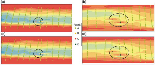
In fact, both the TPS and OKA methods have similar performance not only on scatter plots, but also on the spatial distribution of errors. Figure 10(a–d) demonstrates an example of spatial error distributions in the UR and LR regions by using OKA and TPS methods, respectively (see detail in figure captions). Different colours of the points represent the magnitude of errors with the same classification used in Figure 9. The points with colours of yellow (rank B), red (rank C) and dark green (rank D) represent the data points with relatively large errors. No matter whether we adopt TPS or OK algorithms, the point locations with huge errors are consistently in similar areas. Furthermore, when the distribution of errors were further examined, it is observed that the occurrence of large errors are coincident with irregular surface or topography with abrupt change, such as adjacent slope between shallow point bars to the river channel. Similar discoveries are also found and reported in some previous studies (e.g. Aguilar et al. 2005; Erdogan 2009).

Figure 10. Spatial distribution of error (points with different colours) in different selected area. The error points in plot (a) and (c) are located in UR region (as Figure 6 indicated) and generated by using the OKA (a) and TPS (c) interpolators; whereas error points in plot (b) and (d) are located in UR region (as Figure 7 indicated) and generated by using OKA (B) and TPS (d) interpolators. The background elevations are trimmed from the interpolated surfaces in Figures 7 and 8 with coincided locations and interpolators. Different colours represent different error ranks as well as the ranges in Figure 9. Similar distribution patterns of huge errors (circled in black dashed lines) are found in the same area with different interpolators.

4.5. Comparisons with other studies

Our ultimate result shows both OK with anisotropic consideration (UK and OKA) and TPS (from RBF) interpolators have the best performance on the cross-sectional data in LMR. This finding is similar to the conclusions from several above mentioned studies (Merwade, Maidment, and Goff 2006; Šiljeg, Lozić, and Šiljeg 2014; Chowdhury et al. 2017; Chen et al. 2018a). All these researches addressed that both geostatistical and deterministic interpolation methods have similar performance on generating bathymetric surface.

If scrutinizing the RMSE results in our study (which is the most common statistical criteria been adopted by all these studies), the RMSE results seem to be slightly higher in comparison to other studies that are previously reviewed (Tables 3 and 4). For example, Curtarelli et al. (2015) found that lowest RMSE value was 0.92 m by using OK method for mapping the bathymetry of an Amazonian reservoir. Moreover, Chowdhury et al. (2017) reported that RMSE value ranged between 0.48 and 0.67 m for both IDW and OKA methods in the lower Athabasca River, Canada. However, although the RMSE values in our study are greater than 1.7 m, which is higher than other study; the maximum depths and range are generally greater; therefore, this is in part a scale factor. Additionally, the RMSE values might be affected by the spacing of points, the type of waterbody, and the resolution of measurement and mapping.

A potential explanation is due to the data configuration. Comparing with the regularly spaced gridded sounding points, the traditional cross-sectional sounding points are considered to be less homogeneous and with huge gaps between every cross-section. Similar patterns could be found in Merwade (2009), the author adopted different interpolation methods and developed the ‘trend sorting’ techniques. Still, this study exhibited that mean RMSE values were higher in Kentucky River (0.7–1.8 m) than all the other study reaches (0.3–0.5 m, including Brazos, Rainwater, King Ranch, Sulphur and Ohio). The spatial arrangement of hydrographic data in Kentucky River was the only one from traditional cross-sections, while all the other hydrographic data were either irregular spacing (Brazos, Rainwater and King Ranch) or regularly spaced gridded data (Sulphur and Ohio). In fact, several previous studies reported that sampling density affected the performance of different interpolation methods, especially for generating a DEM (e.g. Aguilar et al. 2005; Chaplot et al. 2006; Erdogan 2009; Guo et al. 2010).

As above mentioned, TIN interpolation was adopted by several studies related to the river bathymetry (i.e., Milne and Sear 1997; Sear and Milne 2000), including one study in LMR (Little and Biedenharn 2014). TIN algorithm extracts vertices data by Delaunay triangulation, and create sets of non-overlapping, contiguous triangles; and combinations of each triangle plane represent the surface morphology. Several studies addressed the densities of sampling point play an important role on the performance of TIN interpolation, higher density tends to obtain better accuracy (Brasington 2000; Guo et al. 2010). However, with immense gaps between cross-sections, our hydrographic dataset might not be a proper format for TIN interpolation. In fact, spurious artefacts (pits and linear feature) were generated while interpolating the sounding points by employing TIN. This phenomenon was observed in previous studies (e.g., McGrath et al. 2007), and it appears that manual modification and visual inspection are required if the TIN method is employed. Thus, similar to most of previous studies summarized in Table 1, we excluded TIN when evaluating interpolation method.

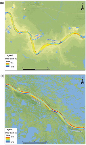
Moreover, although the final results show that OKA and TPS algorithms are adequate interpolators for constructing reliable bathymetric surfaces, the TPS algorithm is comparatively simple to program and implement. In contrast, the OKA interpolator requires anisotropic consideration, which is more complex and computationally inefficiency. Hence, the final bathymetric maps (Figure 11) were constructed by merely using TPS method in UR and LR reaches. Note that the bathymetric maps were converted back from channel-centred (s, n) coordinates to the original Cartesian (x, y) coordinate with each grid has a 10 m × 10 m spatial resolution.

Figure 11. Bathymetric maps of UR region (a) and LR region (b) by using the TPS interpolator in Cartesian (x, y) coordinate system. The spatial resolution of these DEMs are at 10 m × 10 m.

This study has numerous implications to dredging and other engineering applications. For instance, dredging costs are typically $17 to $26 per m³ (Randall et al. 2000). Estimating bathymetry as accurately as possible is essential in order to maintain appropriate river depths for navigation, and obtain bids on contracts for dredging. Inaccurate estimates might end up leaving dredging requirements unmet, or result in unexpected expenditures to complete work as required. In LMR reach, the dredging had been reported as a major engineering activity; with the annually dredging volume reached 13 × 10⁶ m³ during 1988–2011 (Little and Biedenharn 2014; Wang and Xu 2018). The dredging activities have been mainly conducted on the riffles (or crossing) between RK 368 to 165 (Baton Rouge to New Orleans) to maintain the channel navigable (Wang and Xu 2018). Thus, accurate river bathymetry plays an important role on dredging. Engineering estimates might be much more off base in areas where the spatial interpolators performed poorly (Figure 10).

5. Conclusions

This study assesses various interpolation methods for estimating river bathymetry in the lowermost Mississippi River. In order to achieve this goal, cross-sectional data were transformed from into a channel-centred (s, n) coordinate system. Subsequently, different interpolation techniques (OK, OKA, UK, IDW, EIDW, RBF and LPI) were evaluated by employing two cross-validation methods (‘leave-one-out’ and ‘split-sample’ methods) and statistical criteria (RMSE, MAE, bias and r²). Amid all the spatial interpolators, both TPS (a type of RBF interpolator, deterministic) and OKA (geostatistical) interpolators produce the best results when interpolating the cross-sectional soundings within two selected reaches (UR and LR regions). Although the UK interpolator also has strong statistical performance, but the resulting surfaces showed a relative fuzzy surface with blur geographic features.

Moreover, interpolators with anisotropic consideration (EIDW, UK and OKA) are slightly better (>5% to 20% reduction in RMSE values) compared to the isotropic interpolation forms (IDW or OK); which suggest the importance of considering anisotropy in the data before applying interpolating procedures. Additionally, although OKA method performs well statistically, due to the complex procedures for choosing adequate parameters, the final bathymetric DEMs are constructed by using TPS interpolator in our study.

Compared with other studies, the RMSE results from our study are relatively high. One possible explanation is the scale of the waterbody examined. Larger depth numbers are likely to produce larger errors. Another possible explanation is the data configuration, as low sampling density with gaps between each cross-section, thus, higher RMSE values are generated. Here, we only used parts of the hydrographic data surveyed in 1975 by USACE, it is strongly recommended to verify our results by using these hydrographic surveys in different years or different locations in the future. This understanding of the hydrographic model could provide better knowledge for decision-makers, such as planners and engineering practitioners.

Acknowledgments

We would like to thank to Dr Venkatesh Merwade from Purdue University, who provides us his knowledge and software to accomplish this study. Also, we would like to thank Dr Yin-Hseun Chen from University of Florida, who provides some guidance related to perform ArcGIS analysis. Finally, we appreciate two anonymous reviewers for critical suggestions that helped us to improve the quality of this manuscript.

Disclosure statement

No potential conflict of interest was reported by the authors.

References

- Aguilar, F. J., F. Agera, M. A. Aguilar, and F. Carvajal. 2005. “Effects of Terrain Morphology, Sampling Density, and Interpolation Methods on Grid DEM Accuracy.” Photogrammetric Engineering & Remote Sensing 71 (7): 805–816. doi:10.14358/PERS.71.7.805.
- Amante, C. J., and B. W. Eakins. 2016. “Accuracy of Interpolated Bathymetry in Digital Elevation Models.” Journal of Coastal Research 76 (sp1): 123–133. doi:10.2112/SI76-011.
- Bello-Pineda, J., and J. L. Hernndez-Stefanoni. 2007. “Comparing the Performance of Two Spatial Interpolation Methods for Creating a Digital Bathymetric Model of the Yucatan Submerged Platform.” Pan-American Journal of Aquatic Sciences 2 (3): 247–254.
- Boreggio, M., M. Bernard, and C. Gregoretti. 2018. “Evaluating the Differences of Gridding Techniques for Digital Elevation Models Generation and Their Influence on the Modeling of Stony Debris Flows Routing: A Case Study from Rovina Di Cancia Basin (North-Eastern Italian Alps).” Frontiers in Earth Science 6: 89. doi:10.3389/feart.2018.00089.
- Brasington, J., B. T. Rumsby, and R. A. McVey. 2000. “Monitoring and Modelling Morphological Change in a Braided Gravel‐Bed River Using High Resolution GPS‐based Survey.” Earth Surface Processes and Landforms 25 (9): 973–990. doi:10.1002/(ISSN)1096-9837.
- Carter, G. S., and U. Shankar. 1997. “Creating Rectangular Bathymetry Grids for Environmental Numerical Modelling of Gravel-Bed Rivers.” Applied Mathematical Modelling 21 (11): 699–708. doi:10.1016/S0307-904X(97)00094-2.
- Chang, K.T., 2006. Introduction to geographic information systems. Boston: McGraw-Hill Higher Education..
- Chaplot, V., F. Darboux, H. Bourennane, S. Leguédois, N. Silvera, and K. Phachomphon. 2006. “Accuracy of Interpolation Techniques for the Derivation of Digital Elevation Models in Relation to Landform Types and Data Density.” Geomorphology 77 (1): 126–141. doi:10.1016/j.geomorph.2005.12.010.
- Chen, C., Y. Li, N. Zhao, B. Guo, and N. Mou. 2018a. “Least Squares Compactly Supported Radial Basis Function for Digital Terrain Model Interpolation from Airborne Lidar Point Clouds.” Remote Sensing 10 (4): 587. doi:10.3390/rs10040587.
- Chen, C., Y. Li, N. Zhao, and C. Yan. 2018b. “Robust Interpolation of DEMs from Lidar-Derived Elevation Data.” IEEE Transactions on Geoscience and Remote Sensing 56 (2): 1059–1068. doi:10.1109/TGRS.2017.2758795.
- Chowdhury, E., Q. Hassan, G. Achari, and A. Gupta. 2017. “Use of Bathymetric and LiDAR Data in Generating Digital Elevation Model over the Lower Athabasca River Watershed in Alberta, Canada.” Water 9 (1): 19. doi:10.3390/w9010019.
- Conner, J. T., and D. Tonina. 2014. “Effect of Cross-Section Interpolated Bathymetry on 2D Hydrodynamic Model Results in a Large River.” Earth Surface Processes and Landforms 39 (4): 463–475. doi:10.1002/esp.v39.4.
- Cressie, N. 1990. “The Origins of Kriging.” Mathematical Geology 22 (3): 239–252. doi:10.1007/BF00889887.
- Crowder, D. W., and P. Diplas. 2000. “Using Two-Dimensional Hydrodynamic Models at Scales of Ecological Importance.” Journal of Hydrology 230 (3): 172–191. doi:10.1016/S0022-1694(00)00177-3.
- Curtarelli, M., J. Leao, I. Ogashawara, J. Lorenzzetti, and J. Stech. 2015. “Assessment of Spatial Interpolation Methods to Map the Bathymetry of an Amazonian Hydroelectric Reservoir to Aid in Decision Making for Water Management.” ISPRS International Journal of Geo-Information 4 (1): 220–235. doi:10.3390/ijgi4010220.
- Declercq, F. A. N. 1996. “Interpolation Methods for Scattered Sample Data: Accuracy, Spatial Patterns, Processing Time.” Cartography and Geographic Information Systems 23 (3): 128–144. doi:10.1559/152304096782438882.
- Deutsch, C. V., and L. Wang. 1996. “Hierarchical Object-Based Stochastic Modeling of Fluvial Reservoirs.” Mathematical Geology 28 (7): 857–880. doi:10.1007/BF02066005.
- Dury, G. H. 1970. “A Re‐Survey of Part of the Hawkesbury River, New South Wales, after One Hundred Years.” Geographical Research 8 (2): 121–132.
- Erdogan, S. 2009. “A Comparision of Interpolation Methods for Producing Digital Elevation Models at the Field Scale.” Earth Surface Processes and Landforms 34 (3): 366–376. doi:10.1002/esp.v34:3.
- Eriksson, M., and P. P. Siska. 2000. “Understanding Anisotropy Computations.” Mathematical Geology 32 (6): 683–700. doi:10.1023/A:1007590322263.
- Fisk, H. N. 1944, “Geological Investigation of the Alluvial Aquifer of the Lower Mississippi River: US Department of the Army”, Mississippi River Commission, vol. 1947.
- Flanagin, M., A. Grenotton, J. Ratcliff, K. B. Shaw, J. Sample, and M. Abdelguerfi. 2007. “Hydraulic Splines: A Hybrid Approach to Modeling River Channel Geometries.” Computing in Science & Engineering 9 (5): 4–15. doi:10.1109/MCSE.2007.99.
- Goff, J., and S. Nordfjord. 2004. “Interpolation of Fluvial Morphology Using Channel-Oriented Coordinate Transformation: A Case Study from the New Jersey Shelf.” Mathematical Geology 36 (6): 643–658. doi:10.1023/B:MATG.0000039539.84158.cd.
- Goovaerts, P. 1997. Geostatistics for Natural Resources Evaluation. Oxford: Oxford University Press on Demand.
- Gramling, R., C. J. Forsyth, and G. Wooddell. 1998. “Expert Informants and Relative Risk: A Methodology for Modeling Waterways.” Risk Analysis 18 (5): 557–562.
- Guo, Q., W. Li, H. Yu, and O. Alvarez. 2010. “Effects of Topographic Variability and Lidar Sampling Density on Several DEM Interpolation Methods.” Photogrammetric Engineering & Remote Sensing 76 (6): 701–712. doi:10.14358/PERS.76.6.701.
- Harmar, O. P., and N. J. Clifford. 2007. “Geomorphological Explanation of the Long Profile of the Lower Mississippi River.” Geomorphology 84 (3): 222–240. doi:10.1016/j.geomorph.2006.01.045.
- Harmar, O. P., N. J. Clifford, C. R. Thorne, and D. S. Biedenharn. 2005. “Morphological Changes of the Lower Mississippi River: Geomorphological Response to Engineering Intervention.” River Research and Applications 21 (10): 1107–1131. doi:10.1002/(ISSN)1535-1467.
- Hilldale, R. C., and D. Raff. 2008. “Assessing the Ability of Airborne LiDAR to Map River Bathymetry.” Earth Surface Processes and Landforms 33 (5): 773–783. doi:10.1002/(ISSN)1096-9837.
- Hudson, P. 2002. “Pool-Riffle Morphology in an Actively Migrating Alluvial Channel: The Lower Mississippi River.” Physical Geography 23 (2): 154–169. doi:10.2747/0272-3646.23.2.154.
- Isaaks, E. H., and R. M. Srivastava. 1989. An Introduction to Applied Geostatistics. New York, NY: Oxford University Press.
- Johnston, K., J. M. Ver Hoef, K. Krivoruchko, and N. Lucas. 2001. Using ArcGIS Geostatistical Analyst. Esri Redlands.
- Kinzel, P. J., C. W. Wright, J. M. Nelson, and A. R. Burman. 2007. “Evaluation of an Experimental LiDAR for Surveying a Shallow, Braided, Sand-Bedded River.” Journal of Hydraulic Engineering 133 (7): 838–842. doi:10.1061/(ASCE)0733-9429(2007)133:7(838).
- Kis, I. M. 2016. “Comparison of Ordinary and Universal Kriging Interpolation Techniques on a Depth Variable (A Case of Linear Spatial Trend), Case Study of the Sandrovac Field.” Rudarsko-Geolosko-Naftni Zbornik 31 (2): 41.
- Knox, R. L., and E. M. Latrubesse. 2016. “A Geomorphic Approach to the Analysis of Bedload and Bed Morphology of the Lower Mississippi River near the Old River Control Structure.” Geomorphology 268: 35–47. doi:10.1016/j.geomorph.2016.05.034.
- Legleiter, C. J., and P. C. Kyriakidis. 2006. “Forward and Inverse Transformations between Cartesian and Channel-Fitted Coordinate Systems for Meandering Rivers.” Mathematical Geology 38 (8): 927–958. doi:10.1007/s11004-006-9056-6.
- Legleiter, C. J., and P. C. Kyriakidis. 2008. “Spatial Prediction of River Channel Topography by Kriging.” Earth Surface Processes and Landforms 33 (6): 841–867. doi:10.1002/(ISSN)1096-9837.
- Li, J., and A. D. Heap. 2008. A review of spatial interpolation methods for environmental scientists. Canberra: Geoscience Australia.”
- Li, J., and A. D. Heap. 2011. “A Review of Comparative Studies of Spatial Interpolation Methods in Environmental Sciences: Performance and Impact Factors.” Ecological Informatics 6 (3): 228–241. doi:10.1016/j.ecoinf.2010.12.003.
- Little, C. D., and D. S. Biedenharn. 2014. “No Title.” Mississippi River Hydrodynamic and Delta Management Study (Mrhdm)-Geomorphic Assessment.
- Matheron, G., 1969. Le krigeage universel. Cahiers du Centre de Morphologie Mathematique. Fontainebleau: École nationale supérieure des mines de Paris.
- McGrath, J. K., J. P. O’kane, K. J. Barry, and R. C. Kavanagh 2007, “Channel-Adaptive Interpolation for Improved Bathymetric TIN”, Proceedings of the 9th International Conference on GeoComputation, Maynooth, Ireland. url: http://www.geocomputation. org/2007/6B-Algorithms_and_Architect ure_2/6B2. pdf. doi:10.1094/PDIS-91-4-0467B
- Meade, R. H. 1996: Riversediment inputs to major deltas. In J. D. Milliman & B. U.Haq (eds.): Sea-level rise and coastal subsidence. Pp. 63-85. Dordrecht: Kluwer Academic Publ.
- Merwade, V. 2009. “Effect of Spatial Trends on Interpolation of River Bathymetry.” Journal of Hydrology 371 (1): 169–181. doi:10.1016/j.jhydrol.2009.03.026.
- Merwade, V., A. Cook, and J. Coonrod. 2008. “GIS Techniques for Creating River Terrain Models for Hydrodynamic Modeling and Flood Inundation Mapping.” Environmental Modelling and Software 23 (10): 1300–1311. doi:10.1016/j.envsoft.2008.03.005.
- Merwade, V. M., D. R. Maidment, and J. A. Goff. 2006. “Anisotropic Considerations while Interpolating River Channel Bathymetry.” Journal of Hydrology 331 (3): 731–741. doi:10.1016/j.jhydrol.2006.06.018.
- Merwade, V. M., D. R. Maidment, and B. R. Hodges. 2005. “Geospatial Representation of River Channels.” Journal of Hydrologic Engineering 10 (3): 243–251. doi:10.1061/(ASCE)1084-0699(2005)10:3(243).
- Milliman, J. D., and R. H. Meade. 1983. “World-Wide Delivery of River Sediment to the Oceans.” The Journal of Geology 91 (1): 1–21. doi:10.1086/628741.
- Milne, J. A., and D. A. Sear. 1997. “Modelling River Channel Topography Using GIS.” International Journal of Geographical Information Science 11 (5): 499–519. doi:10.1080/136588197242275.
- Mitášová, H., and L. Mitáš. 1993. “Interpolation by Regularized Spline with Tension: I. Theory and Implementation.” Mathematical Geology 25 (6): 641–655. doi:10.1007/BF00893171.
- Moskalik, M., P. Grabowiecki, J. Tęgowski, and M. Żulichowska. 2013. “Bathymetry and Geographical Regionalization of Brepollen (Hornsund, Spitsbergen) Based on Bathymetric Profiles Interpolations.” Polish Polar Research 34 (1): 1–22. doi:10.2478/popore-2013-0001.
- Mossa, J. 1996. “Sediment Dynamics in the Lowermost Mississippi River.” Engineering Geology 45 (1–4): 457–479. doi:10.1016/S0013-7952(96)00026-9.
- Nittrouer, J. A., M. A. Allison, and R. Campanella. 2008. “Bedform Transport Rates for the Lowermost Mississippi River.” Journal of Geophysical Research: Earth Surface 113: F3. doi:10.1029/2007JF000795.
- Nittrouer, J. A., J. Shaw, M. P. Lamb, and D. Mohrig. 2012. “Spatial and Temporal Trends for Water-Flow Velocity and Bed-Material Sediment Transport in the Lower Mississippi River.” Geological Society of America Bulletin 124 (3–4): 400–414. doi:10.1130/B30497.1.
- Panhalakr, S. S., and A. P. Jarag. 2016. “Assessment of Spatial Interpolation Techniques for River Bathymetry Generation of Panchganga River Basin Using Geoinformatic Techniques.” Asian Journal of Geoinformatics 15: 3.
- Parker, G., and S. Ikeda 1989, “River meandering.”
- Philip, G. M., and D. F. Watson. 1982. “A Precise Method for Determining Contoured Surfaces.” The APPEA Journal 22 (1): 205–212. doi:10.1071/AJ81016.
- Pinter, N., and R. A. Heine. 2005. “Hydrodynamic and Morphodynamic Response to River Engineering Documented by Fixed-Discharge Analysis, Lower Missouri River, USA.” Journal of Hydrology 302 (1–4): 70–91. doi:10.1016/j.jhydrol.2004.06.039.
- Randall, R., B. Edge, J. Basilotto, D. Cobb, S. Graalum, Q. He, and M. Miertschin 2000, “No Title”, Texas gulf intracoastal waterway (GIWW) dredged material: beneficial uses, estimating costs, disposal analysis alternatives, and separation techniques.
- Sear, D. A., and J. A. Milne. 2000. “Surface Modelling of Upland River Channel Topography and Sedimentology Using GIS.” Physics and Chemistry of the Earth, Part B: Hydrology, Oceans and Atmosphere 25 (4): 399–406. doi:10.1016/S1464-1909(00)00033-2.
- Shen, Y., and P. Diplas. 2008. “Application of Two- and Three-Dimensional Computational Fluid Dynamics Models to Complex Ecological Stream Flows.” Journal of Hydrology 348 (1): 195–214. doi:10.1016/j.jhydrol.2007.09.060.
- Shepard, D. 1968, “A Two-Dimensional Interpolation Function for Irregularly-Spaced Data”, Proceedings of the 1968 23rd ACM national conference ACM, pp. 517.
- Sherwood, C. R., D. A. Jay, R. B. Harvey, P. Hamilton, and C. A. Simenstad. 1990. “Historical Changes in the Columbia River Estuary.” Progress in Oceanography 25 (1–4): 299–352. doi:10.1016/0079-6611(90)90011-P.
- Šiljeg, A., S. Lozić, and S. Šiljeg. 2014. “A Comparison of Interpolation Methods on the Basis of Data Obtained from A Bathymetric Survey of Lake Vrana, Croatia.” Hydrology & Earth System Sciences Discussions 11: 12. doi:10.5194/hessd-11-13931-2014.
- Smith, S. L., D. A. Holland, and P. A. Longley. 2005. “Quantifying Interpolation Errors in Urban Airborne Laser Scanning Models.” Geographical Analysis 37 (2): 200–224. doi:10.1111/gean.2005.37.issue-2.
- Talmi, A., and G. Gilat. 1977. “Method for Smooth Approximation of Data.” Journal of Computational Physics 23 (2): 93–123. doi:10.1016/0021-9991(77)90115-2.
- Tomczak, M. 1998. “Spatial Interpolation and Its Uncertainty Using Automated Anisotropic Inverse Distance Weighting (Idw)-Cross-Validation/Jackknife Approach.” Journal of Geographic Information and Decision Analysis 2 (2): 18–30.
- Trevisani, S., M. Cavalli, and L. Marchi. 2010. “Reading the Bed Morphology of a Mountain Stream: A Geomorphometric Study on High-Resolution Topographic Data.” Hydrology and Earth System Sciences 14 (2): 393–405. doi:10.5194/hess-14-393-2010.
- Vetter, M., B. Hfle, G. Mandlburger, and M. Rutzinger. 2011. “Estimating Changes of Riverine Landscapes and Riverbeds by Using Airborne LiDAR Data and River Cross-Sections.” Zeitschrift Fr Geomorphologie, Supplementary Issues 55 (2): 51–65. doi:10.1127/0372-8854/2011/0055S2-0045.
- Wang, B., and Y. J. Xu. 2018. “Decadal‐Scale Riverbed Deformation and Sand Budget of the Last 500 Km of the Mississippi River: Insights into Natural and River Engineering Effects on a Large Alluvial River.” Journal of Geophysical Research: Earth Surface 123(5): 874-890.doi:10.1029/2017JF004542
- Xie, Y., T. Chen, M. Lei, J. Yang, Q. Guo, B. Song, and X. Zhou. 2011. “Spatial Distribution of Soil Heavy Metal Pollution Estimated by Different Interpolation Methods: Accuracy and Uncertainty Analysis.” Chemosphere 82 (3): 468–476. doi:10.1016/j.chemosphere.2010.09.053.
- Yang, J., R. D. Townsend, and B. Daneshfar. 2006. “Applying the HEC-RAS Model and GIS Techniques in River Network Floodplain Delineation.” Canadian Journal of Civil Engineering 33 (1): 19–28. doi:10.1139/l05-102.
- Zar, J. H. 1999. Biostatistical AnalysisEdgewood Cliffs, New Jersey: Prentice-Hall.