Hydrologic changes of Aral Sea: A reveal by the combination of radar altimeter data and optical images

ABSTRACT

Aral Sea has gone through a drastic shrinkage during the past century, from more than 68,000 km² in 1960s to less than 10,000 km² in 2015. The desiccation was highly severe in 2009 and 2014 due to the west basin changed to an exposed bottom for several months. Then dust storms, fishery recession and degraded plant communities followed, causing tremendous environmental problems and economic deteriorations. In this paper, high frequency water extents of Aral Sea during 2000–2015 were delineated by MODIS images. Water level changes of the lake were analyzed according to a water level database, which was derived on TOPEX/Poseidon, Jason-1, Jason-2, ENVISAT and SARAL altimeter data. Water volume changes during the same period were determined by a combination of lake surface extents and the corresponding water level data. The largest area of Aral Sea was 30,256.46 km² in May 2000, and the smallest was 6926.04 km² in November 2014. Water storage declination for the whole lake was up to 74km³ and water level dropped from 43.42 m to 39.73 m during 2000–2015. In a whole, west and east basins of the lake presented declination trends (−191.73 km²/yr and −1089.48 km²/yr), while the north basin showed a little increase with the rate of 38.18 km²/yr. For the three basins (north, west and east), corresponding level tendencies were 0.15 m/yr, −0.5 m/yr, −0.38 m/yr, and volume variations were 0.29 km³/yr, −1.36 km³/yr, −3.25 km³/yr, respectively.

KEYWORDS:

• Aral Sea
• radar altimeter
• inundation changes
• water storage

1. Background

As a typical inland saline lake, Aral Sea is located in the adjacent region of Southern Kazakhstan and Northern Uzbekistan (33.0°-48.5°N, 53.5°-79.0°E, Figure 1). The watershed of Aral Sea includes parts of Tajikistan, Turkmenistan, Kyrgyzstan and Afghanistan. Aral Sea was the fourth largest lake in the world before 1960s, with an area of more than 68,000 km² (Micklin 2007). While in 2007, its area was only about one third of 50 years ago and the water volume lost 90% (Micklin 1988, 2007). It experienced a large variability in the last century, and this issue was considered as the world’s largest environmental disaster. Since 1960s, the former Soviet government acclaimed to promote crop plantation and some huge irrigation projects were carried out. The projects mainly drained water from the two feeding rivers Amu Darya and Syr Darya in the watershed. This event broke the original water balance of Aral Sea watershed and caused the continuous declination of its water level, which dropped from an average of 52m in 1780–1960 to less than 40m in nearly 1980 (CAWATERinfo 2016). After that, Aral Sea continued to desiccate until it was splitted to two disconnected parts, North Aral Sea and South Aral Sea (including east and west basins). The east and west basins were connected by a narrow channel, which was always dried up or with a little water since 2000. In 2007, Aral Sea was divided into three separate parts: the north, west and east basins.

Figure 7. Area, level and volume changes for three Aral Sea basins during 2000–2015.

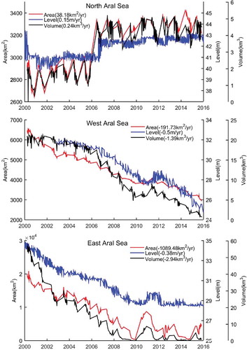
Figure 1. Aral Sea watershed with MODIS bands 2, 1, 4 acquired in July 2000.

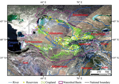
With the shrinkage of shorelines, the local ecosystem, sediment and micro-paleontological situation continually transformed to be negative. Aral Sea became more unsustainable and caused a loss of fish and wild animals, soil salinization, and finally a reduction of cropland production. Additionally, the large area of exposed seabed in east basin was contributed to salty and dusty air, which polluted the Aral Sea region (Micklin 2007). This economic-ecosystem-economic event was recognized as a typical short-sighted anthropogenic activity. In addition, the climate of the watershed is typically desert-continental. Monthly precipitation is approximately 5–25 mm and most of the rainfall occurred in the period of June-August. Temperature of this region is usually −35–10°C in winter and 7–45°C in summer (CAWATERinfo 2016). The main source of the two input rivers are meltwater from glaciers and snow nearby Tien Shan and Pamir mountains during spring-summer, when is favourable for the downstream cropland irrigation.

To better understand Aral Sea’s hydrologic changes, Moderate-resolution Imaging Spectroradiometer (MODIS) images with a 8-day frequency during 2000–2015 were employed to delineate the changes of lake surface area. Database for Hydrological Time Series of Inland Waters (DAHITI) derived from radar altimetry data was used to explore changed details of water level. Aral Sea storage changes were computed based on the series of area and level datasets. Finally, a comprehensive illustration of the changes was present.

2. Data and methods

2.1. Data

2.1.1. Radar altimeter database

Altimeter data is in the form of footprints, recording the measurements on the ground tracks. Altimeter missions are loaded on satellites and emit pulses to the earth. The Range between satellite and the water surface can be calculated by counting the time taken by the pulses to return (Bronner et al. 2013). Thus the height of water surface based on some reference ellipsoid is equal to Altitude of missions subtracts Range (Formula (1)). While the Range needs to be corrected based on various environmental and geophysical corrections (Formula (2)).

(1) $SeaSurfaceHeight=Altitude-CorrectedRange$(1)

(2) $CorrectedRange=Range+wettropospherecorrection+drytropospherecorrection+ionospherecorrection+electromagneticbias$(2)

Among the widely applied altimeter data, TOPEX/Poseidon (T/P), Jason-1, Jason-2, Environmental Satellite (Envisat) and Satellite with ARgos and ALtika (Saral) are radar altimeter data. The emitted pulses of them are microwave pulses, which can take all-weather measurements. While the other kind of emitted pulses is laser pulse, which is easily interfered by clouds and Ice, Cloud and Land Elevation Satellite (ICESat) data is of this kind.

T/P (launched in August, 1992 and ended in October, 2005), Jason-1 (launched in December 2001), and Jason-2 (launched in 2008) missions operated on the same orbit with the ground footprints of about 3–4km in diameter, and covered the latitude of ±66.15 degree, with a repeat cycle of about 9.9 days (AVISO 2016). As a successor of European Remote Sensing satellites (ERS), Envisat was launched in March, 2002 by the European Space Agency (ESA). Envisat covered the latitude of ±81.5 degree, with the footprints around 2 ~ 10km in diameter and the revisit period is 35 days. Envisat stopped working on 8 April 2012, and then Saral reoccupied the same ground tracks from 2013 onwards (ESA 2016). ICESat was also widely used in water level derivation of inland water bodies, especially small lakes due to the diameter of its ground footprints was only 70m. However, the obvious limitation is that its accessibility is only during 2003–2009 (http://nsidc.org/data/icesat/data_releases.html). Overall, there are more than 20 years of altimeter data can be used to capture the level changes of inland lakes. Extensive researches have applied multi-mission altimeter data on the derivation of inland water level (Birkett 1995; Crétaux and Birkett 2006; Crétaux et al. 2009).

In the present, four kinds of altimeter databases have comprehensively made use of the aforementioned altimeter data to determine time series of water level of large river and lakes/reservoirs in the world. The databases are Database for Hydrological Time Series of Inland Waters (DAHITI) (Schwatke et al. 2015), Global Reservoir and Lake Monitor (GRLM) (Birkett et al. 2011), River Lake Hydrology product (RLH) (River and Lake Product Handbook v3.5 2009) and Hydroweb (Crétaux et al. 2011). DAHITI was used in this research to display water level changes of Aral Sea.

DAHITI includes 457 major lakes/reservoirs and rivers in the world and its accuracy was 4 ~ 36cm, depends on surface extents and geographical conditions. The accuracy was obtained according to comparison with gauged observations. Considering radar echoes maybe contaminated by land, ‘off-nadir’ effects occasionally existed and the input altimeter data were with different path locations and accuracies (AVISO 2016), individual waveform retraction, outlier rejection and Kalman filter were carried out for footprints in DAHITI to improve the accuracy of water level derivation. Specific details of the processing procedure were illustrated in research (Schwatke et al. 2015). In DAHITI, the number of water level records for north, west and east basins during 2000–2015 were 759, 277, and 615 respectively. There were not many altimeter data available for the west part, due to the measurements for that region started on 15 June 2002. In addition, DAHITI was in WGS-84 elevation reference.

2.1.2. In-situ observations

To check the accuracy of DAHITI on Aral Sea, historical in situ observations of water level were downloaded from the Database of Aral Sea (CAWATERinfo 2016), while these data for North and South Aral sea were only available during 2000–2006. In addition, the elevation reference of this data was unknown. The observed water volume during 2000–2010 (Gaybullaev, Chen, and Gaybullaev 2012) for North Aral Sea and South Aral Sea were used to compare with the result derived in this research.

2.1.3. MODIS images

The 3rd level composited MODIS product data with 8-day frequency and 500 m resolution in the research period were employed to detect surface extent dynamics. The starting date of the images was 2000–049 and the ending date was 2015–361. They were downloaded from the Earth Observing System at https://reverb.echo.nasa.gov/reverb/. The images included 7 bands from the visible to near-infrared (NIR) wavelength (0.62–2.13 μm) and has been atmospherically corrected (Vermote, Kotchenova, and Ray 2011). However, the fifth band (1.23–1.25 μm) was abandoned because of repetitive stripe noises, and hence the left six bands were used for the next data processing. Usually, there were 46 useful images per year, while some images were contaminated by thick clouds or ice/snow in winter. Therefore, only 310 images in total during 2000–2015 were processed in this research.

2.1.4. Precipitation data

The precipitation data used in this paper are called Climate Data Record (PERSIANN-CDR), which is estimated from Remotely Sensed data using Artificial Neural Networks. CDR is a daily rainfall dataset with the resolution of 0.25°, and its coverage is from 60°S to 60°N. The available CDR is from 1983 to present (Hsu et al. 1997). This dataset can be freely downloaded from ftp://data.ncdc.noaa.gov/cdr/persiann/files/. Yearly CDR during the studied period was made use of to produce the trend map of the watershed.

2.1.5 GRACE data

Gravity Recovery And Climate Experiment (GRACE) missions are twin satellites launched in March 2002 (Tapley et al. 2004). It aims to measure detailed Earth’s gravity field, which can guide gravity and natural system discoveries (http://www.csr.utexas.edu/grace/). GRACE data are in monthly scale, with the spatial resolution of 1° and covers the whole globe. The value of each pixel in GRACE is ‘Liquid Water Equivalent Thickness’, in the unit of cm. The accuracy of this equivalent water height estimate is approximate 1–2 cm (Swenson, Wahr, and Milly 2003; Wahr et al. 2004; Wahr, Swenson, and Velicogna 2006). GRACE data have been widely used to estimate water mass trends in continental scale based on water balance and hydrological models (Güntner 2008; Ramillien et al. 2005; Seitz, Schmidt, and Shum 2008; Werth et al. 2009; Singh, Seitz, and Schwatke 2012). Three solutions of GRACE were supplied by Jet Propulsion Laboratory (JPL), the Center for Space Research at the University of Texas, and the German Research Center for Geosciences. There was a slight difference among them to present water mass changes, and JPL-GRACE was used in this research to analyze.

2.2. Inundation delineation

Many researchers have used normalized difference water index (NDWI) (McFeeters 1996), modified NDWI (MNDWI) (Xu 2006) and automated water extraction index (AWEI) (Feyisa et al. 2014) to extract water because of their simplicity and directness. However, these water indexes are all replied on suitable thresholds to get correct outcomes. Thresholds tend to be diverse for different images because the difference in image acquirement dates, illumination situations and clouds contaminants. Thus, an unique threshold was not suitable for the MODIS images in this study and to determine the suitable threshold for each image is very challenging. Considering the long-time series of MODIS images, the supervised classification method would be more applicable. In this study, the widely used Support Vector Machine (SVM) algorithm and a proposed training set collection method were used to classify MODIS images. As a statistical learning theory derivation, SVM can separate classes with a decision surface, which maximizes the margin between two classes (Vapnik 1982). The surface is usually named optimal hyper-plane and samples located closest to the hyper-plane are called support vectors, and these vectors are the critical elements of training data. Though SVM is a binary classifier in its simplest form, it can be used to classify multiply classes by creating a binary classifier for each possible pair of classes (Hsu, Chang, and Lin 2003). SVM has been widely used in the classification of remote sensing images (Huang et al. 2008; Mountrakis, Im, and Ogole 2011; Song and Civco 2004) and various researches verified its promising because it can achieve higher accuracy than other classifiers such as Maximum Likelihood Classifier, C4.5 (Quinlan 1986, 1993) etc (Cao, Chen, and Imura 2009; Gong et al. 2013；Sun et al. 2014). The present study was conducted using the SVM algorithm with radial basis function kernel included in ENVI (Mountrakis, Im, and Ogole 2011).

As a result of MODIS images were with lower spatial resolution, details of many land cover types cannot be clearly revealed due to mixed pixels. Considering the aim of the research is to distinguish water and no water, a simple classification system was defined including six general classes: water bodies, bare soil and buildings, vegetation, ice, snow, and clouds. Moreover, vegetation includes forest, grassland, and shrub, and bare soil includes impervious area because of the similar reflectance patterns among them.

The goal of this research is to capture the dynamic inundation changes of 8-day interval during the last 16 years. High frequency MODIS data were used to capture the seasonal and inter-annual changes, thus a lot of training data was required to differentiate water and no water. If training data can be selected automatically for each image, then the data processing would be highly efficient. Automatic collection of training data was proposed and it included two steps: (1) A set of initial training data were selected according to the constructed rule sets; (2) an iterative clustering method based on k-means clustering was applied to refine the initial training sets to remove noises. Figure 2 explicitly shows the flow chart of water training sets selection. Considering the diversity of each land cover in MODIS images, the rule sets were defined fully considering the variety of each land cover. For example, clear, green and turbid water were defined to include typical and sufficient water training sets. The establishment of the rule sets and the suggested thresholds were based on the research (Sun et al. 2014). Because the rule sets were created according to experiences and each land cover was with great diversity, it was inevitable that some noises existed. Therefore, an iterative clustering method was explored to refine the initial training sets.

Figure 2. Flowchart of water extraction. The procedure in small red rectangles was the same as that of the large red rectangle.

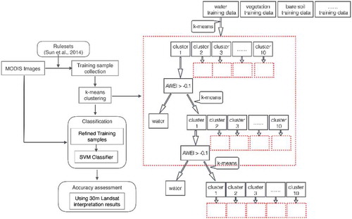
K-means clustering algorithm was carried out iteratively to remove error training samples. As the classification system of this research contained six types, iterative k-means clustering was applied on each training sets separately. The cluster number of each iteration was set to 10. Taking water training dataset as an example, in the first iteration, 10 clusters of water were created. AWEI value of each cluster was calculated to determine whether this cluster was typical water or not. If AWEI of some cluster was greater than −0.1, then this cluster was considered as typical water training sets. While on the contrary, the cluster was clustered to 10 clusters again. After several iterations, if some cluster still not met the condition, then it was excluded from water training sets. Iteration terminated when the total distance of k-means clusters was the minimum. For each cluster, to guarantee the correctness, outlier rejection was performed in each cluster based on the absolute deviation around the mean value. For other land cover training sets, the same process was performed to remove water sets from them. If after several k-means iterations, there was some cluster with AWEI greater than −0.1 in no-water training sets, then this cluster was excluded from the no-water training samples. The threshold −0.1 of AWEI was determined by statistics on large volume of typical and comprehensive water pixels. As Aral Sea is with large area, after iterative k-means clustering, the refined training data was still with a large volume. To improve the process efficiency, the filtered training sets of each type were chosen to reduce data volume according to their distribution in spectral space. The flow chart of water training sets refining is in Figure 2. Other land cover training samples were processed using the similar procedure to remove water out.

310 water extents of Aral Sea were mapped. Water extraction results of shorelines were finally checked visually to verify their correctness and avoid some errors caused by thin clouds, frozen state, or other unexpected circumstances. The extraction results were evaluated by the interpreted water maps. China has produced two sets of global water distribution based on 30m Landsat images acquired around the year 2000 and 2010 (Liao et al. 2014). For Aral Sea, 4 to 8 Landsat images interpretation results were mosaicked to get a clear picture of the lake extent. MODIS classification results of this research were selected according to the acquisition time and scope of the used Landsat images to ensure that the two kinds of images captured the same state of Aral Sea. 30m interpretation results were resampled to 500 m and pixel-by-pixel accuracy assessment was performed. The omission errors were 0.9%, 1.5% and the commission errors were 2.94%, 4.23% for 2000 and 2010, respectively. As the interpreted water maps were with higher accuracies (96%) (Liao et al. 2014), the accuracy of MODIS extraction results in this research should be nearly 90%.

2.3. Water volume calculation

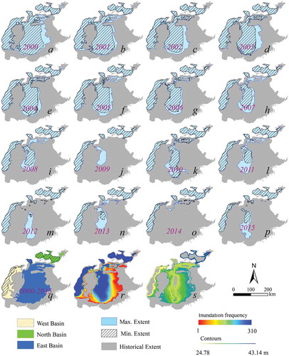
When coastlines of the dynamic extents were determined, each coastline can be treated as a topography contour line (Figure 4(s)). With the aid of the corresponding water level derived from altimeter data, the bottom topography of Aral Sea was modelled by the Triangulated Irregular Network (TIN), which represents the three dimensional surface consisting of a volume of irregularly shaped, linked and non-overlapping triangles (Liu and Mason 2016). There were 759, 277, and 615 water level records in DAHITI, respectively for north, west and east basins. In order to match the 310 coastlines on acquisition dates, 279, 125 and 198 contours were respectively selected to create TIN of the bathymetry map. Besides, the created bathymetry map was based on water level and extent data since 2000. Contours under the smallest surface area during 2000–2015 were unknown. Hence, the calculated water storage was only the changes compared to the minimum extent of Aral Sea during the research period. Moreover, the bottom topography under the smallest extent was assumed unchanged during 2000–2015. Aral Sea experienced tremendous declination, though the exposed seabed may cause salt and dust storms when dust and mineral materials were mixed into air, the changes of the bottom topography can be ignored when compared with the large area of the seabed. Regarding water storage calculation, the elevation value of some water boundary was extracted according to being overlapped on the derived lake bathymetry map. Then the water surface elevation map was created by Kriging interpolation on the vertices (Feng et al. 2011; Wu and Liu 2015). Finally, the water volume was determined from the difference between the interpolated elevation of the surface and the bottom and storage changes were analyzed by the series of water volume data.

Figure 4. Maxima and minima Sea surface extent for the past 16 years of 2000–2015 (a-q), Inundation Frequency map (r) and contour map (s).

3. Results

3.1. Water level changes

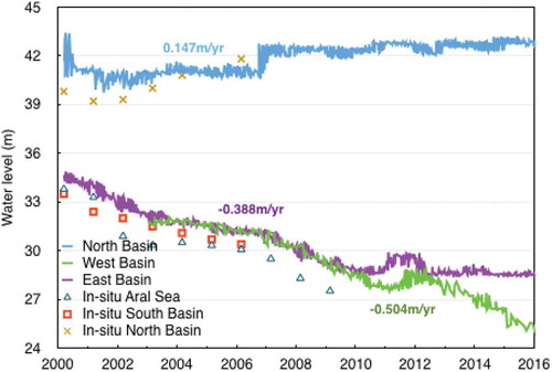
In the case of Aral Sea, results derived by DAHITI were compared with the historical in-situ water level during 2000–2009 (CAWATERinfo 2016) as Figure 3 shows. As the in-situ observations showed, north basin was 39.80 m in 2000 and fluctuately increased to 41.80 m in 2006, while south basin gradually decreased from 33.50 m to 30.40 m in the same period. According to the curves in Figure 3, the dynamic trends of the three basins were similar to the in-situ data though some differences existed. Due to the specific time of the in situ measurements and the vertical datum of the observation station were unclear, the offset of the two datasets can be accepted. The in-situ data showed Aral Sea displayed a clear decreasing trend during 2000–2009. Though the research results, water level of north basin varied from 39.728 m to 43.419 m during 2000–2015 and presented an overall increasing trend (0.147 m/yr). Water level increasing was noticed for north basin since 2006. The east basin water level showed a declination trend from about 35 m in 2000 to 28.447 m in 2015 with a decrease rate of −0.388m/yr. However, West basin dropped 7.315 m in the period of 2002–2015 with a greater rate of −0.504m/yr.

Figure 3. Comparison between In-situ water level (2000–2009) and DAHITI for Aral Sea, North Basin and South Basin, which includes west and east parts.

3.2. Inundation changes

Figure 4(a–q) shows the maximum and minimum annual extents of Aral Sea in the 16-year period, and the corresponding values were listed in Table 2. The ratio of maximum and minima results during 2000–2015 was 4.37 as Figure 4(q) indicates. North basin experienced a slight increasing tendency. With the aid of the Dam constructed in the south of north basin, the north lake showed its stability and was with a little increase by more than 150 km² since 2006. However, both the west and east basins presented a clear decreasing trend. The west decreased gradually at a rate of −191.73 km²/yr due to it is less shallow. As a shallow bottom bathymetry, the recession of east basin was tremendous. The maximum area of the west was 6550.20 km² in April 2000 and the minimum area was 2948.07 km² in October 2015. The spatial extent of the east basin was getting smaller year-by-year with a rate of −1089.48 km²/yr. The narrow channel connecting both of the west and the east was often dried up, causing Aral Sea was divided into three separate parts (the north, the west and the east) since June 2007.

Table 1. In situ hydrological observations of Aral Sea during 2000–2010.

	Water level (m)			Water volume (km^3)
Year	In-situ Aral Sea	In-situ North Basin	In-situ South Basin	In-situ North Basin	In-situ South Basin
2000	33.80	39.80	33.50
2001	33.30	39.20	32.40	17.90	131.20
2002	30.90	39.30	32.00	18.40	110.80
2003	30.34	40.00	31.50	19.80	97.20
2004	30.51	40.80	31.09	22.40	93.50
2005	30.33	41.00	30.70	22.50	89.80
2006	30.08	41.80	30.40	24.00	81.30
2007	29.51			23.20	81.10
2008	28.31			23.00	80.10
2009	27.53			22.80	79.20
2010				22.60	75.50

Table 2. The max. and min. area in each year of 2000–2015.

	2000	2001	2002	2003	2004	2005	2006	2007
The max (km^2)	30,256.46	26,602.26	24,079.61	24,431.76	22,275.74	21,201.27	19,227.13	17,427.57
The min (km^2)	24,584.58	22,956.33	19,776.82	20,772.41	18,972.04	17,199.27	15,785.34	12,407.32
	2008	2009	2010	2011	2012	2013	2014	2015
The max (km^2)	14,659.38	10,285.18	15,894.26	14,841.18	11,712.99	11,978.1	7844.98	11,481.54
The min (km^2)	10,808.69	7390.57	13,487.59	9624.53	7952.33	7903.86	6926.04	8411.51

To get a better view of the spatial inundation fluctuation, all the available 310 water extent maps were overlaid to present the dynamic details of each part, shown in Figure 4(r) with the inundation frequency ranging from 1 to 310. The frequently inundated regions mainly focused on the north basin, the west basin and the north part of the east basin, as the dark blue colour indicates. For east Aral Sea, the inundation frequency decreased gradually from the central to the edge, with the maximum value 287 and the minimum 1. The main body of east Aral Sea retreated to a small pond with an area of around 500 km² in 2009 and was totally exposed as seabed for 7 months in 2014. The west basin experienced a gradual shrinkage with a frequency of 310 in the main body to 1 in the edge. Most of the north basin was frequently covered by water. The wetland and water competed with each other in northeast part of the north basin, leading to the inundation frequency ranged from 1 to 298.

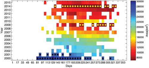
Figure 5 illustrates the inundation area and the occurrence dates in each year. Aral Sea experienced a significant intra-annual variation in the past 16 years. The maxima area of Aral Sea reached to 30,256.46 km² in May 2000 and the minimum inundation area was 6926.04 km² in November 2014. While in 2015, the situation got a little better. Figure 5 suggests that the available 310 data mainly occurred during March-November due to frozen state or snow-covered situation in winter. It is notable that all the available 21 inundation areas in 2014 were recorded as minimum, and 9 of 15 surface extents in 2009 were also donated by black points, as the main body of east basin was totally dried up in several months of these two years.

Figure 5. Area of Aral Sea and the occurrence dates. The interval of x-axis is 16 days. The black points represent 10% of the largest values, and the yellow points denote 10% of the smallest values.

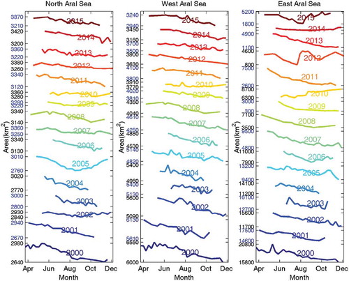
The curves in Figure 6 present fluctuations of the three basins in each year. A small expansion of the north basin is shown by the increases in annual maxima and minima extents since 2006. The annual maxima of north basin during 2000–2005 was up to 3020km² and annual minima was usually less than 2800km². While the annual maximum inundation extent of north basin increased to 3380km² during 2006–2015 and the minimum area of these years was greater than 3130 km². The west basin was shrinking with decreasing annual maxima and the retreating magnitude was stronger during 2000–2008 than the left years. For east basin, the spatial extent was getting smaller year by year and the change pattern in 2014 was more flat due to the disappearance of the main body. The difference between yearly maximum and minimum inundations of the east basin was from 5671 km² in 2000 to 918 km² in 2014, signifying a serious declination.

Figure 6. Intra-annual area changes of Aral Sea during 2000–2015. The y axis indicates the annual extent and the pairs of values in the same colour (blue or black) imply the yearly maximum and minimum inundations.

3.3. Water volume changes

Water storage changes during 2000–2015 was determined based on the interpolated bathymetry map, surface extent and water level data. The water volume variations were the changes compared to the minimum extent in the past 16 years. Figure 7 displays the water storage changes of each basin and their relationships with the corresponding surface area and water level.

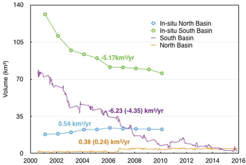
Figure 8. The comparison between in situ water storage changes (2000–2010) and the studied results about the North Bain and South Basin, which includes west and east parts.

For the three separate basins, area, level and volume variation curves are in great agreement with each other, suggesting the close relationships among ongoing hydrological situations of the lake. The expansion of North Aral Sea in the study period was only 777.36 km², and hence the increase of its storage was from 1 to 6 km³, with the rate of 0.24 km³/yr. At the end of 2005, the east-northern of the north basin began drying and disappeared temporarily. But the situation recovered with a complete construction of the dam at the southeast of the north basin during 2005–2006, when the inflow from Syr Darya could not flexibly flow to the east basin. There was a slight increase in water level and area since 2007, and it became stable in the following years. The expansion of the north basin was very small with an area of only up to about 100km² before 2006, while the water volume increased about two times after the Dam construction completed in 2006.

West Aral Sea is comparatively steeper than the east part, and hence the topography isobaths were intensive (Figure 4(s)) and the volume declination was with less intensity. The west basin retreated gradually from 6550.20 km² in 2000 to 2948.07 km² in 2015, and the level dropped from 32.094 m to 24.78 m. The volume of west basin decreased by 20 km³, with a rate of −1.39 km³/yr. East Aral Sea is a comparably shallow lake, connected with the west part through narrow tributary. With the decrease of the supplementary, this part became an isolate one in 2007. The east basin experienced a severe desiccation. In 2000, it was 20,846.74 km², and the water level was 35 m. While in 2009 and 2014, it became a whole exposed seabed, and the situation recovered slightly in 2015. The difference between minimum area and maximum area of east basin was 20517 km² in the study period and the drastic storage changes ranged from 58.23 km³ in 2000 to 0.26 km³ in 2012 with a rate of −2.94 km³/yr.

Figure 8 shows the gauged observations in Table 1 and the research results. The research results were the comparative volume changes relative to the minimum extent during 2000–2015, thus they were much less than the absolute observation volumes.

The historical water volume of the south basin (including west and east parts) was 131.20 km³ in 2001, while in 2010, the value decreased to 75.50 km³, with a decline rate of −5.17 km³/yr. Based on the research result, recession rates of south basin were −6.23 km³/yr during 2001–2010 and −4.35 km³/yr during 2000–2015. From 2000 to 2010, the difference of changing magnitude of south basin between these two datasets was only 1.06 km³/yr. For north basin, the volume raised from 17.90 km³ to 22.60 km³ with a slight increase rate of 0.56 km³/yr based on field measurements during 2000–2010. The research results indicate the change rate of north Aral Sea was 0.38 km³/yr during the same period and the corresponding increment was 4.38 km³, while its increasing rate during 2000–2015 was 0.24 km³/yr. In respect to the total storage of Aral Sea, based on hydrological observation data, the decrease of water volume was 51.00 km³ in 2000–2010, with a shrinkage rate of −4.61 km³/yr. While the studied result shows the volume changes of the whole lake from 2001 to 2010 is 59.55 km³, with a decreasing rate of −5.85 km³/yr. Slight differences on changing rates and decreased volumes relative to the observation measurements indicate that studied results are convinced.

4. Discussion

Some research analyzed precipitation trends of the Aral Sea watershed over 1980–2010 and found that there was no clear change (Zmijewski and Becker 2014). In this research, the relationship between rainfall and the volume changes of Aral Sea was analyzed on the basis of yearly CDR data during 2000–2015, shown in Figure 9.

Figure 9. Trend map of precipitation in the watershed (a), the corresponding volume of precipitation in local Aral Sea region (indicated by the red rectangle in a) and the studied water volume changes of Aral Sea (b).

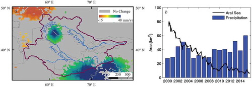
From 2000 to 2015, the trend of precipitation was insignificant in most of the watershed, and rainfall increased in southeast of Aral Sea and in the southern watershed, up to 48mm/yr (Figure 9(a)). In order to analyze the contribution of precipitation, equivalent water volume of precipitation in the local Aral Sea region and the water storage changes were displayed in Figure 9(b). The local Aral Sea region was defined by the maximum historical extent, with an area of 139801 km². Total precipitation in the local Aral Sea region was from 27.48 km³ to 59.94 km³ and presented a fluctuation without an overall trend. The relatively large rainfall data happened in 2003, 2013 and 2015. In 2014, the rainfall was the local minimum, which resulted in the smallest Aral Sea area in the 16 years. However, rainfall was larger in 2009 than its neighbouring years though Aral Sea was also in a smaller extent in 2009. The variation of rainfall was largely different from the contraction of Aral Sea, resulting in that there was no obvious relation between rainfall and Aral Sea storage changes.

Trend map of GRACE water equivalent depth during 2000–2015 was analyzed in Figure 10(a). Majority of the watershed was with negative trends, up to −2cm/yr and the declining magnitude from southeast to northwest was getting stronger. Fluctuations of water loss derived by GRACE were contributed to several hydrological factors, such as rainfall, evaporation, surface and ground water, inflow, soil moisture and so on. Total water loss for the entire basin (1744182 km²) and local Aral Sea region (139801 km²) based on GRACE were compared with water storage changes of the lake (Figure 10(b)).

Figure 10. Trend map of GRACE water equivalent depth in the watershed (a), water volume changes estimated through GRACE data for watershed and local Aral region (indicated by the red rectangle in a) during 2002–2015 and the studied water volume changes of Aral Sea (2000–2015). Watershed volume variance is indicated through blue line and based on the right blue y axis (b).

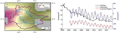
The two GRACE results were in greatly consistent with each other and the three curves coincide well, suggesting the studied result was more reliable. Decreasing trend of overall water mass for the whole watershed from 2000 to 2015 was about −15.47 km³/yr. GRACE curves showed clear seasonality and anomalous dry environments in 2009 and 2014 and this coincided with the performance of the lake. The changed value of GRACE volume in the watershed was up to 210 km³ per month. The corresponding GRACE equivalent water masses for the entire watershed and the local Aral Sea region both displayed overall negative trends during 2002–2015 with a slight recovery in 2010–2012 because of large amounts of snow or rain (Zmijewski and Becker 2014).

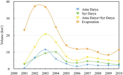
Runoff of the two inflowing rivers and the regional evaporation during 2001–2010 showed that they had an influence on the variation of Aral Sea hydrological changes. During 2001–2010, the runoff of the two feeding rivers fluctuated and presented an overall declination, especially since 2003 (Figure 11). The total runoff of Amu Darya and Syr Darya was 3.10 km³ in 2001 and greatly increased to 20.60 km³ in 2003. From then the discharge gradually decreased to 4.50 km³ in 2010. Changes of the two feeding rivers implied water consumption on the upstream, maybe as a result of the irrigation project or the various small reservoirs constructed by the nearby countries. The observed evaporation increased from 2001 to 2003 and gradually decreased until 2010 in the period of 2001–2010, showing a similar pattern with the river runoff. An increase of the evaporation should be attributed to inefficient irrigation in the Aral Sea region (Zmijewski and Becker 2014). As more than 80% supply of the two inflowing rivers were replenished by the snow and glacier melt (Dukhovny and Schutter 2011), climate change could influence the water depletion of the Aral Sea. The retreat of the glacier on the surrounding mountains may cause reduce in runoff to the Aral Sea (Sorg et al. 2012). Some research found that only ~13.7% of the shrinkage of Aral Sea between 1958 and 2002 was impacted by climate change (Aus der Beek, Voß, and Flörke 2011). Additionally, there was a robust warming trend over Central Asia (World Bank Group 2014; Increasing 2012; Donat et al. 2013), so reduction in surface water flow could be caused by increased evaporation due to higher temperatures (World Bank Group 2014). Besides, Aral Sea watershed has experienced a great increase in population and the irrigated agricultural lands in the past 50 years. The population in Aral Sea Basin increased from 14.1 million in 1960 to 60.4 million in the period of 2007–2012. The irrigated cropland area increased from 4.5 million ha in 1960 to 8 million ha in 2012 and the corresponding withdrawal water rose from 60.6 km³/yr to 105 km³/yr. With the expanded irrigation, newly created reservoirs and the raised evaporation, water use balance was destroyed and then led to sea depression. In the meantime, total runoff to Aral Sea dropped from 55 km³/yr to 10.6 km³/yr (United Nations Environment Programme, 2014).

Figure 11. Hydrological observation data (2001–2010) of Aral Sea (Gaybullaev, Chen, and Gaybullaev 2012).

After Soviet Union collapsed in 1991, there are five countries located around Aral Sea watershed. The relocation of water resource is of vital importance to various economic aims and politic profits. The nearby countries had different influences on the retreat of the sea from their own perspectives. Some reservoirs have been constructed (Figure 1), and they cut the runoff reaching Aral Sea. As a top worldwide producer in cotton (USDA-Foreign Agriculture 2013), Uzbekistan continued to emphasize on cotton export to promote economics and hence the situation of the south Aral Sea presented continued depression. In addition, there was a dam, about 110 km to the south of Amu Darya to compound water. In Kazakhstan, cotton was of slight importance in its economy, while water consumption increased as the local population expanded a lot in mid-1990s. In order to maintain water consumption, Kazakhstan built a 13 km Kok-Aral Dam since 2005 at the southeast coast of the north basin to compound all of the Syr Darya’s discharge. This construction recovered the fishery of the north basin region in the following years (Brilliant Maps 2016). As the most important source, water caused serious conflict in Central Asia. Amu Darya and Syr Darya are trans-boundary rivers, and they are the disputed centre for water demands among Central Asia countries. Kyrgyzstan and Tajikistan, located in the upstream of Syr Darya and Amu Dary rivers, occupied majority of surface water resources (75.20% and 73.99%, respectively) in the two river basins. These two countries are eager to construct large-scale hydropower plants for electricity, while downstream states (Uzbekistan, Kazakhstan and Turkmenistan) rely heavily on water for irrigation (Konur Alp Kocak 2015).

The recession of the sea resulted in severely economic, social and ecological consequences which cannot be recovered. The piped water programs funded by World Band have been carried out in Uzbekistan and Kazakhstan since 1996 (Bakhtior 1998). As there are still many unlined canals, the withdrawal water may be lost before reaching the cropland, causing soil salinization and agriculture production decrease. With the depression of surface extent and salinization of water, the biological productivity was lost. Native fish species dropped greatly and Aral fishery cost higher as the fish went from the seashore to the centre of the lake. The decrease of water level led to fishery companies bankruptcy and the lost of wild animals (Micklin 2007). Moreover, Syr Darya and Aum Darya river delta ecosystems have been deteriorated as river flow diminished, and this may result in disappearance of some small lakes, degradation of plant communities, and spreading of the desert. The local climate may also change with warmer summer, cooler winter, lower humidity and shorten growing season.

5. Conclusions

This paper presented the application of remote sensing techniques on hydrologic delineation of Aral Sea. A novel method of training data automatic selection was proposed and the 310 series of water extraction were processed with high efficiency and accuracy. Based on the water level derived by altimeter data and the corresponding coastlines, topography bathymetry was constructed, and water storage changes of Aral Sea were computed in high temporal frequency. Three dimensional hydrological conditions were presented in this research and with high convince when compared with gauged measurements. Aral Sea experienced drastic shrinkage during the last 16 years. The west and east basins shrunk greatly and the north basin fluctuated and kept stable after 2006. The largest area was 30,256.46 km² in 2000 and the smallest is 6926.04 km² in 2014, it dropped by 23,330 km². The corresponding water storage decrease was 74.84 km³. The main body of east basin went through disappearance in 2009 and 2014 for several months, resulting in nearly 18,236 km² was exposed. The different recession intensity between the west and east basins was that water supply of the east basin was from the north basin and the south Amu Darya river. Human activities of dam construction cut down water supplementary and the narrow tributary connecting the west part and the east part dried up in 2007, making West Aral Sea be an isolate one. This separation may cut the influence of dryness on the west part. Moreover, East Aral Sea was a comparably shallow lake, and West Aral Sea was comparatively steeper, thus water reduction can cause obvious extent recession for the east part.

The analyzed results showed that there was no obvious relation between hydrologic changes of Aral Sea and precipitation variation, thus this conclusion strengthened the impact of human actions. GRACE changes in the watershed showed agreement with Aral Sea volume changes and this illustrated that though Aral Sea was much smaller than the region, the desiccation influenced much larger area. The performance of Aral Sea was dominated, and the whole hydrologic situation of watershed was pessimistic. The recession of the sea led to economic loss in the entire Aral Sea region and hurt the local profit of the inhabitants. Research forecasted that the lake would be 75.40 km³ in 2031 (Gaybullaev, Chen, and Gaybullaev 2012) and some research suggested diverting water from western Siberia into Aral Sea to preserve it (Micklin 2007). Water management among the adjacent countries should be implemented according to protocols to prevent the final dryness of the whole south basin. Sustainable plan should be carried on to provide minimum supplementary to Aral Sea to prevent its disappearance.

Acknowledgements

This paper is financially supported by the State Key Development Program for Basic Research of China (Grant No. 2012CB417006), supported by National Natural Science Foundation of China (Grant Nos. 51190090 and 41171020), Distinguished Young Scholars Fund of Nanjing Forestry University, and Supported by Open Research Fund Program of State Key Laboratory of Water Resources and Hydropower Engineering Science (Grant No. 2011B079) and Key laboratory of watershed Geographic Sciences, Chinese Academy of Sciences (Grant No. WSGS2015005), the State Key Laboratory of Satellite Ocean Environment Dynamics, Second Institute of State Oceanic Administration, Six talent peaks project in Jiangsu Province (Grant No. 2015‑JY‑017) and the Priority Academic Program Development of Jiangsu Higher Education Institutions (PAPD). We would like to thank the National Climate Centre in Beijing for providing valuable help in this research.

Disclosure statement

No potential conflict of interest was reported by the authors.

Additional information

Funding

This work was supported by the National Natural Science Foundation of China [41171020,51190090];Key laboratory of watershed Geographic Sciences, Chinese Academy of Sciences [WSGS2015010];Scientific Program of Guangzhou Bureau of Education [1201430672];Open Research Fund Program of Key Laboratory of Tibetan Environment Changes and Land Surface Processes, Chinese Academy of Sciences[TEL201601].

References

- Aus der Beek, T., F. Voß, and M. Flörke. 2011. “Modelling the Impact of Global Change on the Hydrological System of the Aral Sea Basin.” Physics and Chemistry of the Earth 36 (13): 684–695. doi:10.1016/j.pce.2011.03.004.
- AVISO. 2016. “AVISO-CNES Data Center.” November. http://www.aviso.oceanobs.com/es/misiones/past-missions/topexposeidon.html
- Bakhtior, A. I. 1998. Aral Sea Catastrophe: Case for National, Regional and International Cooperation, the Slavic Research Center.
- Birkett, C. M. 1995. “The Contribution of TOPEX/POSEIDON to the Global Monitoring of Climatically Sensitive Lakes.” Journal of Geophysical Research: Oceans 100: 25179–25204. doi:10.1029/95JC02125.
- Birkett, C. M., C. Reynolds, B. Beckley, and B. Doorn. 2011. “From Research to Operations: The USDA Global Reservoir and Lake Monitor.” In Coastal Altimetry, edited by S. Vignudelli, A. Kostianoy, P. Cipollini, and J. Benveniste, 19–50. Berlin Heidelberg: Springer Verlag.
- Brilliant Maps. 2016. “The Incredible Shrinking Aral Sea 1960-2014.” November. http://brilliantmaps.com/aral-sea/
- Bronner, E., A. Gulliot, N. Picot, and J. Noubel. 2013. SARAL/AltiKa Products Handbook. CNES, France.
- Cao, X., J. Chen, and H. Imura. 2009. “A SVM-based Method to Extract Urban Areas from DMSP-OLS and SPOT VGT Data.” Remote Sensing of Environment 113: 2205–2209. doi:10.1016/j.rse.2009.06.001.
- CAWATERinfo. 2016. “Database of the Aral Sea.” November. http://www.cawater-info.net/aral/data/index_e.htm
- Crétaux, J. F., and C. Birkett. 2006. “Lake Studies from Satellite Radar Altimetry.” Comptes Rendus Geoscience 338: 1098–1112. doi:10.1016/j.crte.2006.08.002.
- Crétaux, J. F., S. Calmant, V. Romanovski, A. Shabunin, F. Lyard, M. Bergé-Nguyen, A. Cazenave, F. Hernandez, and F. Perosanz. 2009. “An Absolute Calibration Site for Radar Altimeters in the Continental Domain: Lake Issykkul in Central Asia.” Journal of Geodesy 83: 723–735. doi:10.1007/s00190-008-0289-7.
- Crétaux J.F., Jelinski W., Calmant S., Kouraev A., Vuglinski V., Berge-Nguyen M., Gennero, M.C., Nino, F., Abarca Del Rio, R., Cazenave, A., Maisongrande P. 2011. “A Lake Database to Monitor in the near Real Time Water Level and Storage Variations from Remote Sensing Data.” AdvancesinSpace Research 4 (7): 1497–1507.
- Donat M.G., Alexander L.V., Yang H., Durre I., Vose R., Dunn R.J.H., Willett K. M., Aguilar E., Brunet M., Caesar J., Hewitson B., Jack C., Klein Tank A. M. G., Kruger A. C., Marengo J., Peterson T. C., Renom M., Oria Rojas C., Rusticucci M., Salinger J., Elrayah A. S., Sekele S. S., Srivastava A. K., Trewin B., Villarroel C., Vincent L. A., Zhai P., Zhang X., Kitching S. 2013. “Updated Analyses of Temperature and Precipitation Extreme Indices since the Beginning of the Twentieth Century: The HadEX2 Dataset.” Journal of Geophysical Research: Atmospheres 118 (5): 2098–2118.
- Dukhovny, V. A., and J. Schutter. 2011. Water in Central Asia-Past, Present, and Future. CRC Press/Balkema: Taylor & Francis Group, London.
- ESA. 2016. “Earth Online.” November. https://earth.esa.int/web/guest/missions/esa-operational-eo-missions/envisat
- Feng, L., C. Hu, X. Chen, R. Li, L. Tian, and B. Murch. 2011. “MODIS Observations of the Bottom Topography and Its Inter-Annual Variability of Poyang Lake.” Remote Sensing of Environment 115: 2729–2741. doi:10.1016/j.rse.2011.06.013.
- Feyisa, G. L., H. Meilby, R. Fensholt, and S. R. Proud. 2014. “Automated Water Extraction Index: A New Technique for Surface Water Mapping Using Landsat Imagery.” Remote Sensing of Environment 140: 23–35. doi:10.1016/j.rse.2013.08.029.
- Gaybullaev, B., S. C. Chen, and D. Gaybullaev. 2012. “Changes in Water Volume of the Aral Sea after 1960.” Applied Water Science 2: 285–291. doi:10.1007/s13201-012-0048-z.
- Gong, P., J. Wang, L. Yu, Y. C. Zhao, Y. Y. Zhao, L. Liang, Z. Niu, et al. 2013. “Finer Resolution Observation and Monitoring of Global Land Cover: First Mapping Results with Landsat TM and ETM+ Data.” International Journal of Remote Sensing 34: 2607–2654. doi:10.1080/01431161.2012.748992.
- Güntner, A. 2008. “Improvement of Global Hydrological Models Using GRACE Data.” Surveys in Geophysics 29 (4–5): 375–397. doi:10.1007/s10712-008-9038-y.
- Hsu, C. W., C. C. Chang, and C. J. Lin. 2003. . “A Practical Guide to Support Vector Classification.” November, 2016. https://www.csie.ntu.edu.tw/~cjlin/
- Hsu, K., X. Gao, S. Sorooshian, and H. V. Gupta. 1997. “Precipitation Estimation from Remotely Sensed Information Using Artificial Neural Networks.” Journal of Applied Meteorology 36: 1176–1190. doi:10.1175/1520-0450(1997)036<1176:PEFRSI>2.0.CO;2.
- Huang, H., P. Gong, N. Clinton, and F. Hui. 2008. “Reduction of Atmospheric and Topographic Effect on Landsat TM Data for Forest Classification.” International Journal of Remote Sensing 29: 5623–5642. doi:10.1080/01431160802082148.
- Increasing, D. A. 2012. “Drought under Global Warming in Observations and Models.” Nature Climate Change 3 (1): 52–58.
- Konur Alp Kocak. 2015. Water Disputes in Central Asia Rising Tension Threatens Regional Stability. European Parliamentary Research Service. http://www.europarl.europa.eu/about-parliament/en/home.
- Liao, A., L. Chen, J. Chen, C. He, X. Cao, J. Chen, S. Peng, F. Sun, and P. Gong. 2014. “High-Resolution Remote Sensing Mapping of Global Land Water.” Science of China, Series D: Earth Science 57: 2305–2316. doi:10.1007/s11430-014-4918-0.
- Liu, J. G., and P. Mason. 2016. Essential Image Processing and GIS for Remote Sensing, 169–170. 2nd ed. New York, USA: Wiley-Blackwell.
- McFeeters, S. K. 1996. “The Use of the Normalized Difference Water Index (NDWI) in the Delineation of Open Water Features.” International Journal of Remote Sensing 17: 1425–1432. doi:10.1080/01431169608948714.
- Micklin, P. P. 1988. “Desiccation of the Aral Sea: A Water Management Disaster in the Soviet Union.” Science 241: 1170–1176. doi:10.1126/science.241.4870.1170.
- Micklin, P. P. 2007. “The Aral Sea Disaster.” Annual Review of Earth Planet. Science 35: 47–72. doi:10.1146/annurev.earth.35.031306.140120.
- Mountrakis, G., J. Im, and C. Ogole. 2011. “Support Vector Machines in Remote Sensing: A Review.” ISPRS Journal of Photogrammetry and Remote Sensing 66: 247–259. doi:10.1016/j.isprsjprs.2010.11.001.
- Quinlan, J. R. 1986. “Induction of Decision Trees.” Machine Learning 1: 81–106. doi:10.1007/BF00116251.
- Quinlan, J. R. 1993. C4.5-Programs for Machine Learning, 81–106. New York: Morgan Kaufman.
- Ramillien, G., F. Frappart, A. Cazenave, and A. Guntner. 2005. “Time Variations of Land Water Storage from an Inversion of 2 Years of GRACE Geoids.” Earth and Planetary Science Letters 235 (1–2): 283–301. doi:10.1016/j.epsl.2005.04.005.
- River and Lake Product Handbook v3.5. 2009. Accessed July, 2017. http://tethys.eaprs.cse.dmu.ac.uk/RiverLake/rl_docs/Product-Handbook-3-05.doc
- Schwatke, C., D. Dettmering, W. Bosch, and Seitz F. 2015. “DAHITI - an Innovative Approach for Estimating Water Level Time Series over Inland Waters Using Multi-Mission Satellite Altimetry.” Hydrology and Earth System Science 19: 4345–4364. doi:10.5194/hess-19-4345-2015.
- Seitz, F., M. Schmidt, and C. K. Shum. 2008. “Signals of Extreme Weather Conditions in Central Europe in GRACE 4-D Hydrological Mass Variations.” Earth and Planetary Science Letters 268 (1–2): 165–170. doi:10.1016/j.epsl.2008.01.001.
- Singh, A., F. Seitz, and C. Schwatke. 2012. “Inter-Annual Water Storage Changes in the Aral Sea from Multi-Mission Satellite Altimetry, Optical Remote Sensing.” And GRACE Satellite Gravimetry Remote Sensing of Environment 123: 187–195. doi:10.1016/j.rse.2012.01.001.
- Song, M., and D. Civco. 2004. “Road Extraction Using SVM and Image Segmentation.” Photogrammetry Engineering and Remote Sensing 70: 1365–1371. doi:10.14358/PERS.70.12.1365.
- Sorg, A., T. Boch, M. Stoffel, O. Solomina, and M. Beniston. 2012. “Climate Change Impacts on Glaciers and Runoff in Tien Shan (Central Asia).” Nature Climate Change, 2(10): 725-731.
- Sun, F., Y. Zhao, P. Gong, R. Ma, and Y. Dai. 2014. “Monitoring Dynamic Changes of Global Land Cover Types: Fluctuations of Major Lakes in China Every 8 Days during 2000-2010.” Chinese Science Bulletin 59 (2): 171–189. doi:10.1007/s11434-013-0045-0.
- Swenson, S., J. Wahr, and P. Milly. 2003. “Estimated Accuracies of Regional Water Storage Variations Inferred from the Gravity Recovery and Climate Experiment (GRACE).” Water Resources Research 39: 8. doi:10.1029/2002WR001808.
- Tapley, B., S. Bettadpur, J. Ries, P. Thompson, and M. Watkins. 2004. “GRACE Measurements of Mass Variability in the Earth System.” Science 305: 503–505. doi:10.1126/science.1099192.
- UNEP (United Nations Environment Programme). 2014. “The Future of the Aral Sea Lies in Transboundary Cooperation.” January.
- USDA-Foreign Agriculture Service, Production Ranking MY. 2013. “National Cotton Council of America.” Accessed November, 2016. http://www.cotton.org/econ/cropinfo/cropdata/rankings.cfm
- Vapnik, V. 1982. Estimation of Dependences Based on Empirical Data. Nauka, Moscow (In Russian). New York: Springer.
- Vermote, E. F., S. Y. Kotchenova, and J. P. Ray. 2011. “MODIS Surface Reflectance User’s Guide.” http://modis-sr.ltdri.org
- Wahr, J., S. Swenson, and I. Velicogna. 2006. “Accuracy of GRACE Mass Estimates.” Geophysical Research Letters 33: L06401. doi:10.1029/2005GL025305.
- Wahr, J., S. Swenson, V. Zlotnicki, and I. Velicogna. 2004. “Time-Variable Gravity from GRACE: First Results.” Geophysical Research Letters 31: L11501. doi:10.1029/2004GL019779.
- Werth, S., A. Güntner, S. Petrovic, and R. Schmidt. 2009. “Integration of GRACE Mass Variations into a Global Hydrological Model.” Earth and Planetary Science Letters 277 (1–2): 166–173. doi:10.1016/j.epsl.2008.10.021.
- World Bank Group. 2014. Turn down the Heat: Confronting the New Climate Normal. Washington, DC: World Bank.
- Wu, G., and Y. Liu. 2015. “Combining Multispectral Imagery with in Situ Topographic Data Reveals Complex Water Level Variation in China’s Largest Freshwater Lake.” Remote Sensing 7 (10): 13466–13484. doi:10.3390/rs71013466.
- Xu, H. 2006. “Modification of Normalized Difference Water Index (NDWI) to Enhance Open Water Features in Remotely Sensed Imagery.” International Journal of Remote Sensing 27: 3025–3033. doi:10.1080/01431160600589179.
- Zmijewski, K., and R. Becker. 2014. “Estimating the Effects of Anthropogenic Modification on Water Balance in the Aral Sea Watershed Using GRACE: 2003–12.” Earth Interactions 18: 1–6. doi:10.1175/2013EI000537.1.