Controlling for spatial confounding and spatial interference in causal inference: modelling insights from a computational experiment

ABSTRACT

Causal inference is a rapidly growing field of statistics that applies logical reasoning to statistical inference to estimate causal relationships. Spatial data poses several problems in causal inference – namely, spatial confounding and interference – that require different strategies when designing causal models. In order to obtain valid inferences, existing nonspatial causal models must adjust for such spatial problems. Given the blossoming literature on spatial causal inference, this research analyzes the usage of spatial causal models under a priori knowledge and a priori ignorance of the spatial structure of data. We synthesize existing research directions in noncausal spatial modelling and causal nonspatial modelling by assessing the performance of 28 spatial causal models across 16 spatial data scenarios. We used ordinary least squares (OLS) models, conditional autoregressive (CAR) models, and jointly CAR models for outcome and treatment variables as the basis for the tested models, equipping them with a variety of spatial causal adjustments. We compare our results to principles of noncausal spatial modelling and investigate their implications for spatial causal modelling. Specifically, we show that noncausal spatial modelling guidance holds in causal spatial modelling workflows and demonstrate how researchers can leverage noncausal theory to great effect. In parallel, we introduce the spycause Python package of spatial causal models and data simulators to facilitate the widespread use of these models and to enable reproduction and extension of our work.

KEYWORDS:

• Spatial causal inference
• spatial confounding
• spatial interference
• modelling guidance

1 Introduction

A central goal of geographic research is to identify and infer causal relationships that govern the spatial processes that shape real-world phenomena, ultimately leading to actionable insights (Harvey 1968; Hernán 2018; Pearl 2000). However, the spatial statistical methods used in many geographic studies do not themselves provide strong evidence of causation (Herrera, Mur, and Ruiz 2014). Rather, commonly applied techniques such as spatial regression are designed to stabilize the estimation of key parameters by including otherwise omitted spatial relations (Anselin 1988; Cressie 1993; LeSage 2014). Those parameter estimates are then given causal interpretations by researchers in light of existing theories and prior evidence. This situation presents spatial analysts with a contradiction: they endeavour to identify causal connections to better explain and affect phenomena in the real world, but often rely on methods that provide limited direct evidence of causation.

To address these issues and more clearly connect statistical evidence to causal arguments, causal inference has emerged as a subfield of statistics focused on the development of methods that model interventions and their potential connection to observed outcomes (Imbens and Rubin 2015; Pearl 2000). Causal inference is distinguished from traditional statistical inference by its application of formal logical rules to lend causal interpretations to statistical quantities. The goal of a causal analysis is to isolate and estimate the effect of a treatment on an outcome variable in the presence of other factors that may complicate this process. While promising, the development of a robust approach to space is still emerging in this literature, leaving the methodological innovations of causal inference open to the well-established critiques of applying non-spatial methods to spatial problems (Gibbons and Overman 2012; Harris, Moffat, and Kravtsova 2011; McMillen 2010). Namely, that it is necessary to alter conventional causal models for estimating causal relationships in spatial applications because geographic processes, and the spatial effects they produce, create spatial dependencies among observations that violate modelling assumptions and require adjustments to avoid biasing parameter estimates and inferences (Paelinck and Mur 2018).

A small but growing body of work in spatial statistics has begun to engage with the causal inference literature (see Akbari, Winter, and Tomko 2021; Gao et al. 2022; Herrera, Mur, and Ruiz 2014; Reich et al. 2021). Much like the development of spatial regression techniques, these scholars are adapting nonspatial causal modelling methods for the analysis of spatial data, resulting in new spatial causal modelling techniques. These techniques address two uniquely spatial forms of known impediments to causal inference.

First, spatial causal models address the issue of spatial confounding, which occurs when a variable at location $i$ affects both the treatment $Z$ and outcome $Y$ variables at another location $j$ (Figure 1b). If the structure of the spatial confounding is known and the confounding variable is observed, then a spatial lag of the confounding variable may be included to adjust for the confounding effects; more complex adjustments are required if the confounding variable is unobserved (Section 2.2). If left unaddressed, spatial confounding biases statistical estimates of relationships among variables and produces inferences that cannot be interpreted causally. For example, residential location spatially confounds the relationship between air pollution and birthweight (Paciorek 2010). Individuals choose to live in places for a variety of factors, including income and ethnicity, that may influence the birthweight of their children. At the same time, an individual’s place of residence exposes them to differing levels of air pollution. As a result, the values of variables like income and ethnicity are spatial confounders of the pollution-birth weight relationship: their values at neighbouring locations may influence both an individual’s exposure to air pollution and the birthweight of their children.

Figure 1. Graphical depictions of (a) nonspatial confounding, (b) spatial confounding, and (c) spatial interference. In nonspatial confounding, confounding variables X affect treatment variables Z and outcome variables Y at the same location (a). Spatial confounding arises when these relationships cross locations (b). That is, $X_i$ takes the role of the confounding variable at location $j$, blocking inference of the effect of $Z_j$ on $Y_j$. Spatial interference occurs when treatment at one location affects outcomes at other locations (c). Adapted from Reich et al. (2021).

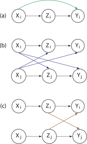
Second, spatial causal models include adjustments for spatial interference, which exists when the treatment variable at location $i$ affects the outcome variable at another location $j$ (Figure 1c). Spatial interference may be a natural consequence of the spatial dependencies that exist between nearby locations (Tobler 1970) and can create violations of the stable unit treatment value assumption (SUTVA). SUTVA is a central assumption of causal inference and holds that one unit of analysis will not affect how another unit of analysis responds to an intervention. Violations of SUTVA, spatial or otherwise, prohibit causal inferences by affecting the outcome variable in ways that are not solely due to the treatment variable (Imbens and Rubin 2015). For example, Zigler and Papadogeorgu (2018) study the impact of installing specialized emissions control systems at coal or natural gas power plants on hospitalization rates for air pollution-related health outcomes. One power plant receiving such a system may affect anyone who resides downwind of the plant; that is, one location receiving treatment may have impacts that spill over to neighbouring locations. This spillover creates spatial interference, as an untreated zip code may receive extraneous treatment or a mixture of treatments from all upwind power plants, altering the outcome variable for that zip code. Using an adjustment for spatial interference, Zigler and Papadogeorgu found that installing the systems at power plants upwind from a zip code, rather than at the nearest power plant to a zip code, led to a greater reduction in hospitalization rates.

While spatial causal models have the potential to strengthen the causal interpretation of statistical evidence in geographic research, these methods have yet to be widely adopted or studied by geographic researchers. Two key factors limiting the development and use of spatial causal models in geography are a lack of familiarity with these techniques and a lack of practical guidance for their application. When modelling, researchers make decisions about spatial structures that affect their inferences and add uncertainty to the modelling procedure. Noncausal spatial modelling can guide these decisions to remedy spatial issues and mitigate the accumulation of uncertainty in modelling procedures. Our experiments interpret this advice in a causal modelling setting to introduce the ideas of spatial causal modelling and to begin building a base of practical guidance for researchers using spatial causal models.

In practice, researchers seldom know whether and to what degree spatial confounding and interference are present in a data generating process. This situation leaves researchers facing uncertainty along two dimensions. First, researchers face uncertainty about the spatial structure of the data generating process and the presence of confounds and interferences. Second, lacking certainty about the structure of the data generating process, researchers face uncertainty as to which model best suits a given circumstance. This uncertainty affords researchers a degree of flexibility when determining the specification of their model. These researcher degrees of freedom (DOFs) (Gelman and Loken 2013; Simmons, Nelson, and Simonsohn 2011) and uncertainties about the world define two axes of a high-dimensional space populated with the (mis)match between models and the data generating processes they seek to represent (Figure 2). By leveraging spatial reasoning in causal inference, geographers may be able to create workflows for spatial causal modelling akin to the workflows for noncausal spatial modelling.

Figure 2. An example matrix of models (rows) and data scenarios (columns) as functions of their parameters. Each entry contains a vector of performance metrics and represents a point in combined parameter space (researcher DOFs and data characteristics).

The noncausal spatial modelling literature contains a rich discussion of principles to guide spatial workflows (Elhorst 2013; Golgher and Voss 2016; LeSage and Pace 2009, 2014). In general, simple, parsimonious models are preferable to complex models, and prior to beginning a spatial modelling analysis, a simple (nonspatial) model should be investigated (Fotheringham, Brunsdon, and Charlton 2002). If a researcher suspects spatial issues may be present, they should employ a conditional or simultaneous autoregressive (CAR or SAR, respectively) model, reserving more powerful models for when the researcher is very confident that the issues are intricate and difficult to untangle (Elhorst 2013). Selecting the right weights matrix for these models is challenging, but researchers must be aware that region-based weights may create more problems than they solve (Hodges and Reich 2010). Finally, the literature advises that researchers make liberal use of spatial and nonspatial diagnostics to ensure that all components of the modelling workflow are behaving as expected (Anselin and Rey 2014).

In this paper, we show that many of these same principles hold in a causal spatial modelling context. Fundamentally, because there is little difference in estimation between causal models and noncausal models, insights and guidance from noncausal spatial modelling should transfer to causal spatial modelling. We establish the usefulness of this advice by testing, validating, and illustrating the relative performance of 28 spatial causal models across 16 spatial data scenarios. To create the data scenarios, we vary the structures of spatial confounding and interference in the data while holding all other parameters constant (Section 2.1). Then, we fit three kinds of models with several different spatial confounding and interference adjustments – an ordinary least squares model (OLS), a conditional autoregressive model (CAR), and a joint CAR model for the propensity score and outcome variables (Joint) – for a total of 28 spatial causal model structures (Section 2.2). The OLS and CAR models are well-studied tools of the noncausal spatial modelling literature, but the joint model is tailored to causal problems: by using a spatial model for the propensity scores that is linked to a spatial model for the outcome variable, the joint model represents a very detailed spatial structure. Moreover, even if spatial confounding and interference in the data are not properly modelled, we find that noncausal spatial modelling principles can guide users towards valid inferences. To facilitate reproducibility and encourage others to build on our work, we develop and share an extensible Python package that contains all data generation and model code, so users can easily create example datasets with spatial and nonspatial confound or interference.

The remainder of the paper is organized into three sections. In Section 2, we introduce the design of our simulation experiments, including the data generating processes and models used. In Section 3, we present the outputs of the simulations and explore their implications for principles of spatial causal modelling and researcher modelling choices. Finally, in Section 4 we highlight key takeaways and turn an eye towards what future work may hold.

2 Experimental design

The central aim of our experiment is to enable wider usage of spatial causal models in geography by demonstrating the operation of these models under an array of data scenarios. Our experiment considers three model forms – an ordinary least squares model, a spatial conditional autoregressive model, and a hierarchical model for the treatment and outcome variables – with a variety of adjustments for spatial confounding and interference. We demonstrate the relative performance of these causal models across our set of experimental results to build a base of practical knowledge about the role of space in causal modelling. As noncausal models differ from causal models in their underlying assumptions rather than in their estimation procedures, we show that noncausal spatial modelling guidance largely holds in the causal spatial modelling setting.

We investigate spatial causal modelling workflows where the researcher has a priori knowledge of the problem’s underlying spatial structures and where the researcher does not have a priori knowledge of the problem’s spatial structures. In the first case, we establish the utility of spatial causal models, anticipating that nonspatial causal models will not correctly estimate average treatment effects in spatially confounded or interfered data. It is possible that under weak spatial confounding, nonspatial causal models will place confounding effects into error terms and these models will perform well despite not explicitly adjusting for the spatial confounding. On the other hand, lacking knowledge of the problem’s spatial confounding or spatial interference may lead to mismatches between spatial structures in the data and in the model that a researcher chooses to apply to the data. If spatial causal models are highly sensitive to these mismatches, then it may be preferable to begin with nonspatial causal models; on the other hand, if some spatial causal models have uniformly superior performance to all nonspatial causal models, they will be preferable as analytical starting points. Among these experiments are simulations that check if spatial causal models properly degenerate to nonspatial models on data without spatial confounding or interference. If this is not the case, then there may be a significant disadvantage to beginning analysis with a spatial causal model.

From the results of our experiments, we construct matrices that capture differing combinations model specifications and data scenarios. Each entry in these matrices holds information about the performance of a set of modelling choices on a set of spatial data characteristics, which we use to examine model behaviour across a variety of data scenarios (Figure 2). Specifically, we consider the bias (accuracy) and the variance (precision) of the estimated parameters as performance metrics of interest: a model performs well on a data scenario if it exhibits low bias and low variance. The next sections define the parameter space of the simulations and describe our modelling approaches.

2.1 Data generating processes (DGPs)

To examine the relative performance of spatial causal models across data generating processes (DGP) subject to different levels of spatial confounding and spatial interference, we developed a simulation strategy centred on the classic triangular confounding graph (Figure 3), which links the effect of treatment $Z$ to outcome $Y$ subject to confounds $X$. We simulated the DGPs on a gridded spatial domain with $N=900$ samples apiece. Then, we introduced spatial confounding and spatial interference into the DGPs via spatial weights matrices, which describe the structure of dependencies between variables. By using four different weights matrices for the spatial confounding and the spatial interference, we were able to examine 16 different DGPs, which then we simulated 28 times to facilitate model comparison for a total of 448 simulations. The full details of our simulation strategy and code to reproduce or replicate our results are available in Appendix A and in the simulation study Github repository. Here, we present the central features of our simulation procedure in five steps.

Figure 3. Data simulation strategy for the experiments. First, constants are fixed (variables outside of boxes; see Appendix a for more information). Next, the confounders $X$ are drawn following the above rules. These are used to generate the treatment variable $Z$ via the propensity score $\pi$. Finally, the confounders and treatment variables are combined to generate the outcome. Note also that this diagram shows the most general possible circumstances – if ${\rho }_{\mathcal{U}}=0$, for example, then there is no spatial confounding present in the data.

First, we created nonspatial confounding variables $X$ that have a modest level of spatial autocorrelation (${\rho }_X=0.9$) in accordance with Tobler’s First Law (Figure 3, top box). This law states that objects are likely to be related to other nearby objects, a feature commonly found in spatial data (Tobler 1970). Second, to introduce spatial confounding, we drw a spatial confounder $\mathcal{U}$ from a conditional autoregressive (CAR) distribution with parameters ${\rho }_{\mathcal{U}}$ and ${\sigma }_{\mathcal{U}}^2$. CAR distributions are commonly used as DGPs for spatially autocorrelated data in simulation studies and applied settings (Banerjee, Carlin, and Gelfand 2015; Cressie 1993). Third, to model the probability of unit $i$ receiving treatment ($P(Z_i=1)$), we defined and calculated the treatment probabilities ${\pi }_i=P(Z_i=1)$. These probabilities, called propensity scores, model the probability of a unit receiving treatment ($Z_i=1$) subject to measured covariates; in this instance the nonspatial confounders $X$, the spatial confounder $\mathcal{U}$, and another CAR term $V$ (independent of $\mathcal{U}$) that models spatial dependence in the treatment allocation beyond $X$ and $\mathcal{U}$ (Reich et al. 2021). Fourth, to make the treatment assignment we then drew the treatment variable as a weighted coin flip using the propensity scores created in step three (Figure 3, left box). For each unit $i$, the probability that $Z_i=1$ was ${\pi }_i$ and the probability that $Z_i=0$ was $1-{\pi }_i$. Fifth, to introduce the effects of spatial interference into the simulation strategy, we use the $N\times 2$ matrix $\tilde{Z}=[Z,WZ]$ in lieu of $Z$ and turn $\tau$ into the two-dimensional vector $[\tau ,\tilde{\tau }]$ where $\tau$ is the prescribed average treatment effect. To facilitate comparison across simulations, the treatment effect was held constant at $\tau =1.5$ and the interference effects were fixed at $\tilde{\tau }=0.5$. This technique allows the presence of a treatment $Z$ in one location to influence the outcome of another location. Finally, we drew the values of the outcome variable $Y$ from a normal distribution as a function of the spatial and non-spatial confounders ($\mathcal{U}$, $X$) and treatment variable ($Z$, or $\tilde{Z}$ if interference is present) (Figure 3, right box).

This simulation strategy allows us to simulate DGP scenarios that reflect a wide variety of spatial and nonspatial confounding and interference scenarios. For example, by setting ${\sigma }_{\mathcal{U}}^2=0$ and $\tilde{\tau }=0.5$, we can investigate a scenario in which spatial interference is present but spatial confounding is not. Similarly, we can control the extent of spatial confounding by varying the spatial weights $W_C$ used to generate $X$, the weights $W_{\mathcal{U}}$ and $W_V$ used to generate the confounding terms $\mathcal{U}$ and $V$, or the weights $W_I$ used to generate the interference. Moreover, because each element is simulated using a different weighting matrix, we can also easily examine different spatial structures for different components of the simulation. In this experiment, we constrained our investigation of both spatial confounding and spatial interference to four alternative weights schemes – no weights (matrix of zeros), binary contiguity (Queen) weights, distance-based ($k$-nearest neighbours) weights, and region-based (predetermined) weights. The combination of four weights matrices for confounding and four weights matrices for interference give a total of 16 data scenarios.

2.2 Model specification

Following Reich et al. (2021), we examined three fundamental model structures: the OLS model, the CAR model, and a joint CAR model for the propensity score and outcome variables (Table 1). The models were fitted using a Bayesian estimation procedure, synthesizing prior information alongside signals from the data to obtain statistical inferences. We begin with the OLS model, which acts as a reference to standard regression procedures. However, we note that OLS cannot directly model spatial confounding because it assumes all observations are independent of each other; the modelling structure does not account for any influence between observations at different locations. We then examine the CAR model – the basis of many noncausal spatial approaches – as it controls for spatial confounding by including a spatially structured error component (Banerjee, Carlin, and Gelfand 2015; Besag 1975; Besag, York, and Mollié 1991; Cressie 1993). Finally, we examine the joint model because it is an approach tailored to causal problems. By using a spatial model for the propensity scores that is linked to a spatial model for the outcome variable, the joint model is able to represents more detailed spatial structure. While more sophisticated spatial causal models (Diao, Leonard, and Sing 2017; Keele and Titiunik 2015; Kolak and Anselin 2020) exist within the literature, we limited our analyses to these three regression adjustments because they remain some of the most commonly applied methods in the spatial literature and afford direct comparison of estimates and performance.

Table 1. The three basic model formulations used for fitting data in the simulation experiment. For more information on the precise structure of a CAR distribution, see Banerjee et al. (2015)..

Name	Model
OLS	$y\sim N(X\beta +Z\tau ,{\sigma }^2)$
CAR	$y\sim N(X\beta +Z\tau +\mathcal{U},{\sigma }^2)$
	$U\sim \mathrm{C}\mathrm{A}\mathrm{R}({\rho }_{\mathcal{U}},{\sigma }_{\mathcal{U}}^2)$
Joint	$y\sim N(X\beta +Z\tau +\mathcal{U},{\sigma }^2)$
	$Z\sim \mathrm{B}\mathrm{e}\mathrm{r}\mathrm{n}\mathrm{o}\mathrm{u}\mathrm{l}\mathrm{l}\mathrm{i}(\pi )$
	$\mathrm{l}\mathrm{o}\mathrm{g}\mathrm{i}\mathrm{t}(\pi )=X\alpha +\varphi \mathcal{U}+V$
	$U\sim \mathrm{C}\mathrm{A}\mathrm{R}({\rho }_{\mathcal{U}},{\sigma }_{\mathcal{U}}^2)$
	$V\sim \mathrm{C}\mathrm{A}\mathrm{R}({\rho }_V,{\sigma }_V^2)$

In total, we tested 28 modelling options: 4 total OLS models with the four kinds of interference adjustment, 12 CAR models with combinations of three kinds of confounding and four kinds of interference adjustment, and 12 joint models with combinations of three kinds of confounding and four kinds of interference adjustment. To adjust for interference in the CAR and joint models, we transform the $N$ dimensional vector $Z$ into the $N\times 2$ matrix $\tilde{Z}=[Z,WZ]$ and reorganize $\tau$ to be a two-dimensional vector whose first element is the average treatment effect. Adding this adjustment accounts explicitly for interference in the model setup, identifying the average treatment effect when interference is present in the data.

All models were fit using a Markov chain Monte Carlo (MCMC) algorithm in the Stan programming language, a probabilistic programming language used for Bayesian inference (Stan Development Team 2021). In Bayesian inference, all statistical parameters are assigned a prior distribution that describes the modeller’s beliefs about the parameter before beginning an analysis. Priors are then combined with a likelihood distribution generated from the data to create a posterior distribution, synthesizing prior belief and real information. In all the models, $\beta$, $\tau$, and $\alpha$ were assigned independent $N(0,2^2)$ priors to let the data drive the inferences. The variance ${\sigma }^2$ was assigned a $\mathrm{E}\mathrm{x}\mathrm{p}\mathrm{o}\mathrm{n}\mathrm{e}\mathrm{n}\mathrm{t}\mathrm{i}\mathrm{a}\mathrm{l}(1)$ prior, putting most of its weight on low values. On the spatial terms, the ${\sigma }_{\mathcal{U}}^2$ and ${\sigma }_V^2$ parameters were transformed into precision parameters and assigned $\mathrm{\Gamma }(0.5,0.005)$ priors, while the ${\rho }_{\mathcal{U}}$ and ${\rho }_V$ parameters were assigned implicit Uniform$(0,1)$ priors. We monitored convergence of the Markov chains to the posterior distributions using standard Bayesian diagnostics, such as counting the number of divergent transitions per chain, computing the effective sample size (ESS), computing $\hat{R}$ scores, or computing the Bayesian fraction of missing information (BFMI). For analysing our results across many simulations, we obtained point estimates of the parameters using the median of their posterior distributions. Summarizing posteriors with point estimates is a common practice in application as well, trading robust inference for quick interpretation (Gelman et al. 2008). More information about the simulation procedure can be found in Appendix A.

3 Results

3.1 Bias and variation in treatment effect estimates across scenario-model combinations

Our main results are presented in Figure 4.¹ Like Figure 2, the horizontal axis of both panels presents the 16 simulated data scenarios defined by variations in the structure of spatial confounding and spatial interference. The vertical axis of both panels presents the 28 the model specifications that we examined. Figure 4a presents the ratio of the bias to the true treatment effect. For each simulation-model combination, we calculated the bias by taking the posterior median of the average treatment effect and calculated the absolute difference between this estimated effect and the true treatment effect. Then, we calculated the ratio of the bias to the true treatment effect size, putting the bias in units of the treatment effect size. This procedure allows us to compare the magnitude of the bias relative to the true magnitude of the treatment effect. If the bias to treatment effect ratio is about 1, then the error in estimating the treatment effect is as large as the treatment effect itself, indicating a high degree of inaccuracy in the model’s inferences. Figure 4b presents the logarithm of the posterior variance for the treatment effect for each scenario-model combination. Models with higher posterior variance are less precise and have more uncertain estimates than those with lower posterior variance. As most of the variances were very small (median 0.008), we used a log transformation to better illustrate the relative ordering of variances across scenario-model combinations.

Figure 4. Throughout, we use the following abbreviations for the kinds of spatial confounding and interference: N corresponds to ‘none’, B is for ‘binary contiguity weights’, D is for ‘distance-based weights’, and R is for ‘region-based weights’. panel (a): ratio of bias to treatment effect size using posterior medians as point estimates for the treatment effect. Low values indicate better model accuracy in capturing the true average treatment effect. Values above 1 imply that the bias is on the same or larger numerical scale as the treatment effect, suggesting that the model is highly inaccurate. For all simulations, the true value of the treatment effect was held constant at 1.5 for comparability. All models perform very well (low bias to effect size ratio) when no spatial confounding is present in the data, but begin to vary in quality with different pairings of spatial confounding and interference in the data. panel (b): logarithm of posterior variance of the treatment effect. The log scale was chosen to better illustrate the differences among simulations: of the untransformed variances, the minimum value was 0.0005, the maximum was 1.064, and the median was 0.008. Low values indicate better model precision and less uncertainty in the posterior distribution for the treatment effect. Most models achieve low variance when no spatial confounding is present, but accrue more uncertainty as spatial confounding takes on different forms.

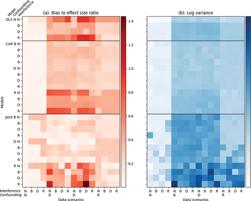
Across all scenario-model combinations, the median bias was 25% of the size of the treatment effect. A total of 43 (9.5%) of scenarios had a bias at least half the size of the treatment effect, while 2 (0.4%) of the scenarios had bias at least as large as the treatment effect. In the worst performing combinations, a distance-based confounding and interference scenario modelled by a joint model specified with region-based confounding and interference, we found bias equal to 1.43 times the size of the treatment effect. In the best performing combination, a no confounding or interference scenario modelled by a CAR model specified with a distance-based confounding adjustment and no interference adjustment, we found bias equal to 0.0008 times the size of the treatment effect. Among combinations where the modelled spatial confounding and interference adjustments matched the data spatial confounding and interference scenarios, the median bias was 24.2% the size of the treatment effect. The biases in these matched scenarios ranged from 0.3% of the size of the treatment effect to 41% of the size of the treatment effect, while the unmatched biases ranged from 0.08% to 143.9%.

Overall, we found that spatial confounding has a more significant impact on model performance than spatial interference (Appendix B). One important feature of Figure 4 is the observable difference between data scenarios with and without spatial confounding – between the first four columns and the remainder of the columns. Across all model specifications, these scenarios produced less bias and variance than the scenarios with spatial confounding because the underlying DGP has less structure. For these scenarios, the CAR and joint spatial models produced similar levels of bias and variance as OLS, indicating that these models degenerate to nonspatial models in the absence of spatial causal issues.

3.2 Guidance for the specification of spatial causal models

We use the results of our simulation experiment to evaluate whether five practices used to guide the specification and estimation of noncausal spatial regression models hold in the spatial causal setting. We find that modelling principles from the noncausal literature hold for spatial causal models. We also present advice on spatial causal model selection when facing uncertainty about unobserved, but potentially spatially structured, DGP.

First, our simulations support the practice of preferring simpler models to complex models in the absence of knowledge about the underlying spatial structures of the DGP (Elhorst 2013; Gibbons and Overman 2012). Figure 4 shows that variance grows primarily as a function of model complexity: CAR models generally exhibit higher posterior variances in the treatment effect estimates than OLS, and joint models generally exhibit higher posterior variances than CAR models. In the absence of any external or prior information about the spatial structure of a dataset, less complex models such as an OLS model with no confounding adjustment, or a CAR specified with a binary confounding adjustment, have only slightly smaller treatment effect variances than more complex alternatives, such as joint models specified with both spatial confounding and interference adjustments. Though treatment effect bias decreases as model complexity increases, it is offset by the increase in treatment effect variance, making inferences more accurate but less certain. While simpler models require stronger assumptions, they are easier to interpret than more complex alternatives as they express more direct relationships between variables and have fewer parameters to estimate. One caveat to this finding is that the sample size of each simulation ($N=900$) may have contributed to higher variance in the joint model. As the joint model has more parameters and represents more complex structures, it requires a larger sample size to attain the same statistical precision as simpler models, making its inferences less useful when data is scarce.

Second, if there is reason to believe the DGP might be structured by spatial confounding or interference, researchers should opt for a spatial model over OLS. The first four columns of Figure 4a show that a CAR model specified with any type of confounding and interference adjustment exhibits lower bias and variance than OLS when the DGP is structured by some forms of spatial confounding. Importantly, OLS may produce invalid inferences if spatial confounding is present in the data. Moreover, CAR models also have low bias even in the absence of confounding, which lowers the penalty for using a CAR model when the DGP is not structured by spatial confounding. In all tested nonspatial scenarios, we found that the CAR model degenerates to a nonspatial model. There is therefore less risk of producing biased estimates when using a CAR model than when using an OLS model if the analyst suspects spatial confounding and interference may be present in the data.

Third, our results suggest that if a strong reason exists to believe the DGP is structured by spatial confounding or spatial interference, a researcher conducting a spatial causal analysis should prefer a joint model to a CAR model. Our experimental results show that a joint model specified with binary spatial confounding has a higher treatment effect variance but less treatment effect bias than CAR models specified with any form of spatial confounding across all spatially confounded scenarios. The higher variance of the joint models is driven by the greater number of parameters included in the model. However, that variance rise is offset by the lower bias produced by the joint model in spatially confounded scenarios due to the model’s inclusion of a propensity score model for the treatment effect. By explicitly modelling the treatment allocation with a spatial component, a joint model can account for the effects of spatial confounders on $Z$ as well as on $Y$. In contrast, CAR and OLS models only account for the effects of spatial confounders on $Y$.

Fourth, region-based weights should only be used in spatial confounding or spatial interference adjustments if a strong reason exists to believe that the spatial confounding or spatial interference in the DGP is structured by regions. Region-based weights group all units within a region as neighbours and exclude all units outside the region, leading to discontinuities at the borders of regions (Figure S1). Even though two units may be nearby in distance, a model using region-based weights for spatial confounding or spatial interference adjustments will not allow the units to affect each other unless they are also in the same region. Moreover, a modifiable areal unit problem (MAUP) issue arises if the regions used for the model’s weights are not the same as the regions of spatial confounding or interference in the data: bias may be incurred from the mismatch between the model’s regions and the data’s regions. Figure 4 shows that modelling non-region-based spatial effects using region-based weights yields high treatment effect bias due to misspecifying the dependencies between units (Anselin and Arribas-Bel 2013). On the other hand, binary- and distance-based adjustments perform equivalently on data experiencing binary- or distance-based spatial confounding and spatial interference (Figure 4). As such, region-based weights should be reserved for data that is highly likely to exhibit region-based confounding or interference—e.g. a county-wide policy affects the response of local corporations to a national regulation – while binary- and distance-based weights should be preferred otherwise (Hodges and Reich 2010; LeSage and Pace 2014).

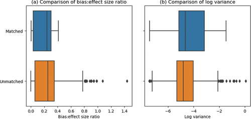
Fifth, it may be difficult post hoc to identify scenarios when the modelled spatial confounding or interference do not match the data spatial confounding or interference. As the true value of an average treatment effect is never known in practice, modellers face a dilemma: it may be impossible to tell when a model outputs a spurious inference. For both the biases and variances, the bulk of the matched and unmatched distributions are located around similar values – although the unmatched scenarios have more outliers (Figure 5). In our simulations, 58% of the unmatched scenarios hit diagnostic flags that indicate poor convergence of the chains to a posterior distribution. Poor convergence is often a symptom of poor model structure and convergence diagnostics signal the researcher to consider different spatial adjustments.

Figure 5. Panel (a): comparison of bias to effect size ratios across matched (data spatial confounding and interference are correctly modelled) and unmatched (data spatial confounding and interference are not the same as modelled spatial confounding and interference) scenarios. $n=28$ in the matched group, $n=420$ in the unmatched group. panel (b): comparison of log variances across matched (data spatial confounding and interference are correctly modelled) and unmatched (data spatial confounding and interference are not the same as modelled spatial confounding and interference) scenarios. $n=28$ in the matched group, $n=420$ in the unmatched group.

4 Conclusion

In this paper, we present the results of a simulation experiment that establishes the relative performance of two approaches to spatial causal modelling across a range of spatially structured data generating processes. Specifically, we compare the bias and variance in treatment effect estimates made by a CAR model adjusted for spatial confounding and spatial interference and a joint model that links a spatial CAR model of propensity scores to a spatial model of treatment outcomes. An OLS model is also included for baseline comparison.

Our results expand our understanding of the performance of spatial causal models under different conditions, give practical advice for spatial causal modelling, and makes emerging research on spatial causal models more accessible to researchers that might use these techniques in geographic applications. By identifying differences in the bias and variance of spatial causal models, our work can also be used to target specific models for improvement in future work. For example, our investigation of region-based weights could be extended to study misspecification error when the modelled regions have different shapes than the regions of spatial confounding or interference in the data. Understanding the sensitivity of spatial causal models to shape and scale issues between regions may further inform model selection. Likewise, developing different representations of spatial dependence beyond the weights matrix may alleviate the bias incurred from misspecification by removing constraints on the model.

It is important to note that causal interpretations of statistical parameters are only valid under the assumptions of the model. The difference between a causal model and a statistical model lies in their identifying assumptions. While all of the parameters in the tested models are statistically estimable, the parameters only have a causal interpretation if all sources of confounding have been controlled in the model. In our simulations, only 28 of the 448 simulations (6.25%) satisfied this condition. In real-world analyses, researchers typically do not know the true causal process or how it is structured by other factors or spatial processes, so models with well-justified assumptions are used to approximate causal inference. This situation not only highlights the importance of the reasoning that underlies a model, but re-emphasizes the value of working with domain experts that can provide context, prior knowledge, for spatial modelling decisions. Leveraging this information is key to ensuring modelled spatial confounding and interference are as closely matched to the data’s spatial confounding and interference as possible, thereby improving approximation of a causal identification. As such an important avenue for future research is to develop a set of best practices for collaborating with domain experts to improve model specification and causal estimation.

Finally, we encourage researchers interested in expanding upon our work to explore the online version of our results matrix in the https://github.com/tdhoffman/spycausespycause-experiments repository and to use the https://github.com/tdhoffman/spycausespycause Python package to further test and improve spatial causal models. The latter package contains all the code needed to simulate data and fit spatial causal models, while the former contains our simulation drivers, data files, and graphical outputs. Tutorialization and documentation are also key components of the spycause package: Jupyter notebooks in the repository demonstrate the use of spatial causal models and act as interactive examples. In this paper, we used only a small portion of the flexibility built into the simulation procedures of the spycause package. Future simulation studies may benefit from varying more parameters, exploring different spatial structures in datasets, and testing a broader range of spatial causal models.

Acknowledgements

This material is based on work supported by the National Science Foundation through a Graduate Research Fellowship awarded to Hoffman under NSF Grant No. 026257-001 and project grant No. BCS-2049837 awarded to Kedron. Any opinions, findings, and conclusions or recommendations expressed in this material are those of the authors and do not necessarily reflect the views of the National Science Foundation.

Disclosure statement

No potential conflict of interest was reported by the authors.

Supplementary data

Supplemental data for this article can be accessed online at https://doi.org/10.1080/19475683.2023.2257788

Additional information

Funding

This material is based on work supported by the National Science Foundation under Graduate Research Fellowship Grant No. 2233001 and Grant No. BCS-2049837.

Notes

1. The full results of the simulations are hosted on the Github repository for this project under outputs.

References

- Akbari, K., S. Winter, and M. Tomko. 2021. “Spatial Causality: A Systematic Review on Spatial Causal Inference.” Geographic Analysis 55 (1): 56–89. https://doi.org/10.1111/gean.12312.
- Anselin, L. 1988. Spatial Econometrics: Models and Methods. Norwell, MA: Kluwer Academic Publishers. https://doi.org/10.1007/978-94-015-7799-1.
- Anselin, L., and D. Arribas-Bel. 2013. “Spatial Fixed Effects and Spatial Dependence in a Single Cross-Section.” Papers in Regional Science 92 (1): 1–17. https://doi.org/10.1111/j.1435-5957.2012.00480.x.
- Anselin, L., and S. J. Rey. 2014. Modern Spatial Econometrics in Practice: A Guide to GeoDa, GeoDaspace, and PySal. Chicago, IL: GeoDa Press, LLC.
- Banerjee, S., B. P. Carlin, and A. E. Gelfand. 2015. Hierarchical Modeling and Analysis for Spatial Data. 2 ed. Boca Raton, FL: CRC Press. https://doi.org/10.1201/b17115.
- Besag, J. 1975. “Statistical Analysis of Non-Lattice Data.” The Statistician 24 (3): 179–195. https://doi.org/10.2307/2987782.
- Besag, J., J. York, and A. Mollié. 1991. “Bayesian Image Restoration, with Two Applications in Spatial Statistics.” Annals of the Institute of Statistical Mathematics 43 (1): 1–20. https://doi.org/10.1007/BF00116466.
- Cressie, N. P. 1993. Statistics for Spatial Data. revised ed. New York: Wiley. https://doi.org/10.1002/9781119115151.
- Diao, M., D. Leonard, and T. F. Sing. 2017. “Spatial Difference-In-Differences Models for Impact of New Mass Rapid Transit Line on Private Housing Values.” Regional Science and Urban Economics 67:64–77. https://doi.org/10.1016/j.regsciurbeco.2017.08.006.
- Elhorst, J. P. 2013. Spatial Econometrics. Berlin: Springer. https://doi.org/10.1007/978-3-642-40340-8.
- Fotheringham, A., C. Brunsdon, and M. Charlton. 2002. Geographically Weighted Regression: The Analysis of Spatially Varying Relationships. Chichester, UK: Wiley.
- Gao, B., J. Wang, A. Stein, and Z. Chen. 2022. “Causal Inference in Spatial Statistics.” Spatial Statistics 50:100621. https://doi.org/10.1016/j.spasta.2022.100621.
- Gelman, A., A. Jakulin, M. G. Pittau, and Y.-S. Su. 2008. “A Weakly Informative Default Prior Distribution for Logistic and Other Regression Models.” The Annals of Applied Statistics 2 (4): 1360–1383. https://doi.org/10.1214/08-AOAS191.
- Gelman, A., and E. Loken. 2013. “ The Garden of Forking Paths: Why Multiple Comparisons Can Be a Problem, Even When There is No “Fishing Expedition“ or “p-hacking“ and the Research Hypothesis Was Posited Ahead of Time. “ Retrieved February 05, 2023. http://www.stat.columbia.edu/~gelman/research/unpublished/p_hacking.pdf. Unpublished.
- Gibbons, S., and H. G. Overman. 2012. “Mostly Pointless Spatial Econometrics?” Journal of Regional Science 52 (2): 172–191. https://doi.org/10.1111/j.1467-9787.2012.00760.x.
- Golgher, A. B., and P. R. Voss. 2016. “How to Interpret the Coefficients of Spatial Models: Spillovers, Direct and Indirect Effects.” Spatial Demography 4 (3): 175–205. https://doi.org/10.1007/s40980-015-0016-y.
- Harris, R., J. Moffat, and V. Kravtsova. 2011. “In Search of ‘W’.” Spatial Economic Analysis 6 (3): 249–270. https://doi.org/10.1080/17421772.2011.586721.
- Harvey, D. W. 1968. “Pattern, Process, and the Scale Problem in Geographic Research.” Transactions of the Institute of British Geographers 45 (45): 71–78. https://doi.org/10.2307/621393.
- Hernán, M. A. 2018. “The C-Word: Scientific Euphemisms Do Not Improve Causal Inference from Observational Data.” American Journal of Public Health 108 (5): 616–619. https://doi.org/10.2105/AJPH.2018.304337.
- Herrera, M., J. Mur, and M. Ruiz. 2014. “Detecting Causal Relationships Between Spatial Processes.” Papers in Regional Science 95 (3): 577–594. https://doi.org/10.1111/pirs.12144.
- Hodges, J. S., and B. J. Reich. 2010. “Adding Spatially-Correlated Errors Can Mess Up the Fixed Effect You Love.” The American Statistician 64 (4): 325–334. https://doi.org/10.1198/tast.2010.10052.
- Imbens, G. W., and D. B. Rubin. 2015. Causal Inference for Statistics, Social, and Biomedical Sciences. New York: Cambridge University Press.
- Keele, L. J., and R. Titiunik. 2015. “Geographic Boundaries as Regression Discontinuities.” Political Analysis 23 (1): 127–155. https://doi.org/10.1093/pan/mpu014.
- Kolak, M., and L. Anselin. 2020. “A Spatial Perspective on the Econometrics of Program Evaluation.” International Regional Science Review 43 (1–2): 128–153. https://doi.org/10.1177/0160017619869781.
- LeSage, J. P. 2014. “What Regional Scientists Need to Know About Spatial Econometrics.” The Review of Regional Studies 44 (1): 13–32. https://doi.org/10.52324/001c.8081.
- LeSage, J. P., and R. K. Pace. 2009. Introduction to Spatial Econometrics. Chapman and Hall/CRC Press. https://doi.org/10.1201/9781420064254.
- LeSage, J. P., and R. K. Pace. 2014. “The Biggest Myth in Spatial Econometrics.” Econometrics 2 (4): 217–249. https://doi.org/10.3390/econometrics2040217.
- McMillen, D. P. 2010. “Issues in Spatial Data Analysis.” Journal of Regional Science 50 (1): 119–141. https://doi.org/10.1111/j.1467-9787.2009.00656.x.
- Paciorek, C. J. 2010. “The Importance of Scale for Spatial-Confounding Bias and Precision of Spatial Regression Estimators.” Statistical Science 25 (1): 107–125. https://doi.org/10.1214/10-STS326.
- Paelinck, J. H., and J. Mur. 2018. “Some Issues on the Concept of Causality in Spatial Econometric Models.” Estudios de Economia Aplicada 36 (1): 107–118. https://doi.org/10.25115/eea.v36i1.2519.
- Pearl, J. 2000. Causality: Models, Reasoning, and Inference. 1 ed. Cambridge, UK: Cambridge University Press.
- Reich, B. J., S. Yang, Y. Guan, A. B. Giffin, M. J. Miller, and A. Rappold. 2021. “A Review of Spatial Causal Inference Methods for Environmental and Epidemiological Applications.” International Statistical Review 89 (4): 605–634. https://doi.org/10.1111/insr.12452.
- Simmons, J. P., L. D. Nelson, and U. Simonsohn. 2011. “False-Positive Psychology: Undisclosed Flexibility in Data Collection and Analysis Allows Presenting Anything as Significant.” Psychological Science 22 (11): 1359–1366. https://doi.org/10.1177/0956797611417632.
- Stan Development Team. 2021. Stan Modeling Language Users Guide and Reference Manual. Accessed February 05, 2023. https://mc-stan.org/. Version 2.28.
- Tobler, W. 1970. “A Computer Movie Simulating Urban Growth in the Detroit Region.” Economic Geography 46:234–240. https://doi.org/10.2307/143141.
- Zigler, C. M., and G. Papadogeorgu. 2018. “Bipartite Causal Inference with Interference.” Statistical Science 36 (1): 109–123. https://doi.org/10.1214/19-STS749.