Land use suitability analysis using an approach combining GIS, regionalization, and PROMETHEE II

ABSTRACT

Land-use Suitability Analysis, which aims to identify the suitability of a given area for a particular use by using a certain number of criteria, is a domain that has received a lot of attention from researchers during the last 20 years and most of the works that have been proposed rely on the use of multi-criteria methods which are based on a complete aggregation of alternatives such as Weighted Linear Combination (WLC). The outranking methods, which are multi-criteria methods that rely on a partial aggregation of alternatives, have rarely been used. In the context of Land-use Suitability Analysis, outranking methods quickly reach their computational limits because they require performing comparisons between each pair of pixels. To reduce the initial number of alternatives, we propose to proceed to the regionalization of the study area by grouping neighbouring pixels that have similar properties in homogeneous zones. We then use PROMETHEE II (Preference Ranking Organization Method for Enrichment of Evaluations), an outranking method whose objective is to rank a set of alternatives from the best to the worst. A study for the choice of a landfill site was carried out using our approach and the obtained results were compared with those of WLC.

KEYWORDS:

• Land-use suitability analysis
• constrained regionalization
• agglomerative hierarchical clustering
• average linkage clustering
• PROMETHEE II

1. Introduction

The objective of land-use suitability analysis is to determine the suitability of a given area for a particular use. For this, each aspect that has been taken into consideration in the analysis (soil permeability, slope of the land, distance from inhabited areas, etc.) is evaluated, separately at first, to see if the area in question whether or not it is suitable for the intended use. Then, all of the assessments made are aggregated to obtain an overall suitability index from which each area is deemed suitable or not. In this type of analysis, it is necessary to consider several potential sites (alternatives) and to measure the impact of each aspect, or criterion, on each alternative in order to then choose the one that best meets the expectations of the competent authorities. Land use suitability analysis is therefore a decision-making problem that has the particularity of being both spatial and multi-criteria.

Given that a good part of decision-making issues are spatial in nature, there is a real need for multi-criteria decision support approaches (MCDA) that pay particular attention to space in the analysis if we want to obtain results that make sense and thus avoid having erroneous recommendations (Malczewski and Rinner 2015). GIS-MCDA approaches (based on the integration of the analytical capacities that characterize GIS with the problem-solving capacities of MCDA where several criteria are usually taken into consideration) constitute a very promising path. In the conventional form of this integration, like GIS-WLC, GIS is often used to score each alternative on each criterion using procedures that exploit the spatial properties of the manipulated data such as proximity analysis, then, a multi-criteria aid method, like WLC, combines the scores obtained for each alternative to calculate an overall index from which each zone is judged to be suitable (to some degree) or not.

Depending on the multi-criteria decision support method used, the GIS-MCDA approaches that have been proposed in the context of land use suitability analysis are divided into two groups: full aggregation-based approaches and partial aggregation-based approaches.

1.1. Full aggregation based approaches

These methods are based on the complete aggregation of the scores obtained for each alternative on each criterion using a so-called utility function. This way of seeing things is based on the assumptions of commensurability and transitivity of the judgements of the decision maker (Mena 2000). The objective of these methods is to establish a complete order on the set of all alternatives. In this context, the land use suitability analysis has benefitted from many examples of GIS-MCDA integration where many multi-criteria decision support methods have been used: Weighted Linear Combination, or WLC (Gbanie et al. 2013), Ordered Weighted Averaging, or OWA (Romano et al. 2015), and compromise programming. Compromise programming is based on two concepts: the definition of a reference point, on one side, and the choice of a distance measure on the other. The reference point is a hypothetical alternative against which the alternatives are evaluated. The distance between a given alternative and a reference point represents the deviation from the ideal solution (Demesouka, Vavatsikos, and Anagnostopoulos 2013). According to Malczewski and Rinner (2015), two methods have emerged from compromise programming: the ideal point method on the one hand, and TOPSIS (Technique for Order Preference by Similarity to the Ideal Solution) on the other (Bagherzadeh and Gholizadeh 2016). is an example of a work using compromise programming.

The common point between all the approaches that rely on a full aggregation multi-criteria decision support method like those cited above (WLC, OWA and compromise programming) is that the overall adequacy index is calculated at the scale of the pixel (considered as being an alternative), a thresholding is then used to discard all pixels whose index of overall adequacy is below a certain value. All the retained pixels are considered to be suitable, to some degree, for the envisaged type of use. The major drawback of these approaches is that the aggregation of the criteria, operating at the level of each pixel, makes them blind to what happens at the level of the other pixels. It is therefore very common to have, using these approaches, small groupings of pixels that can be described as very suitable but which are surrounded by pixels that are not very suitable and vice versa.

1.2. Partial aggregation based approaches

Methods that rely on partial aggregation of criteria are also called outranking methods. Contrary to methods that are based on a full aggregation of criteria, leading to the establishment of a total order on the alternatives, the outranking methods, including ELECTRE (ÉLimination Et Choix Traduisant la REalité) and PROMETHEE (Preference Ranking Organization Method for Enrichment of Evaluations) methods, have been designed to reproduce the preference model of the decision maker by bringing out situations such as weak preference, and sometimes incomparability between alternatives. These situations can result from uncertainties, conflicts or contradictions that characterize the decision maker’s preference model when faced with a particular decision problem (Roy and Bouyssou 1993). Partial aggregation of criteria relies on the construction of outranking relations to represent the global preferences on the different alternatives. The construction of these relations is based on pairwise comparison of actions and on verifying for each pair of alternatives (a, b) whether a outranks b or whether b outranks action a. Comparison between actions is made possible using discrimination thresholds on preference, indifference, and sometimes on veto, which are chosen according to the preferences of the decision maker on criteria that are not necessarily all quantitative and whose performance can be expressed using different units of measure. Unlike methods which are based on a complete aggregation of criteria, outranking methods are not compensatory because a low performance on one criterion cannot be compensated by a high performance on another criterion. However, it should be noted that the outranking methods that deal with the problem of ranking are not immune to the so-called rank-reversal problem because the order of preference may change when an alternative is added to or removed from the decision problem.

In the context of land-use suitability analysis, the integration of outranking methods in a GIS environment has mainly been reserved for analyzes done in a vector format in which a relatively small number of alternatives have been evaluated (Vavatsikos, Demesouka, and Anagnostopoulos 2020). In the following sections, we present the characteristics of the main methods of outranking that have been used in the context of land use suitability analysis.

1.2.1. PROMETHEE II

The objective of the PROMETHEE II method is to rank the alternatives from the best to the worst using a complete pre-order accepting situations of indifference and strict preference only. The ranking of the alternatives is obtained by performing the following steps (Brans and De Smet 2016):

• Calculation of global preference indices: for each pair of actions (a, b), an overall preference index, π (a,b), is calculated based on pairwise comparisons where the deviation between the evaluations of two alternatives on a particular criterion is considered. This index measures the degree of preference of action a over action b with respect to all the criteria.

• Calculation of outranking flows: for each action a, a set of quantities are calculated. These quantities refer to the following flows:

  • Positive outranking flow ɸ⁺(a): representing the power of action a, and measuring the degree to which a outranks all other alternatives.

  • Negative outranking flow ɸ⁻(a): representing the weakness of action a, and measuring the degree of outranking of action a by the other actions.

  • Net outranking flow ɸ(a): representing the difference between the positive and the negative flows.

• Ranking of the alternatives: Once φ is calculated at each alternative, the pre-order of the alternatives can be obtained. φ plays the same role as that of the utility function in establishing the final ranking.

Thanks to its simplicity, PROMETHEE II has been used in many works dealing with land use suitability analysis (Dehghan et al. 2021; Sotiropoulou and Vavatsikos 2021). and (Vavatsikos, Sotiropoulou, and Tzingizis 2022) are some examples.

1.2.2. ELTRE TRI

ELECTRE Tri, one of the methods of the ELECTRE family, proposes to assign a set of alternatives to a set of categories that have previously been defined (Good alternatives, Average alternatives and Bad alternatives for example). This allocation is based on the comparison of the alternatives with so-called reference actions which define the conditions that the performances must meet for an action to be allocated to one category rather than another. The assignment of an action a to a category is carried out by respecting the following points (Roy and Bouyssou 1993):

• The categories are ordered from the one intended to receive the worst alternatives to the one intended to receive the best alternatives.

• Each category C^h is defined using two reference actions: b^h-1 and b^h, one defining the low profile of the category, the other its high profile. C^h is intended to contain actions a such that a is preferred to b^h-1, and b^h is preferred to action a.

• If an action a, which we wish to assign to a particular category, is indifferent to a reference action b^h, then a must be assigned to the class higher than b^h, i.e. C^h+1.

The assignment of the alternatives to the different categories can be done using a conjunctive procedure, or a disjunctive procedure. In the case of a conjunctive procedure, each action a is assigned to the largest value of h such that a S b^h-1. In the opposite case, i.e. a disjunctive procedure, each action a is assigned to the smallest value of h such that b^h S a. In either case, the outranking relation used in ELETRE Tri is based on the calculation of a credibility index, σ, between the actions that one wishes to affect and the profiles of reference.

ELETRE Tri is based on a simple approach allowing it to assign the alternatives to a set of categories. In addition to that, the assignment procedure is based on the comparison of actions with the reference profiles and not on the comparison of actions with themselves, which makes it possible to use ELECTRE-Tri even when the number of alternatives is high.

1.2.2.1. Main works

To reduce the computational load caused by the need to compare each pair of alternatives Joerin et al (2001), Marinoni (2006), Chakhar and Mousseau (2008) propose to form areas from neighbouring pixels sharing similar properties. To achieve this end, Joerin et al (2001) used an iterative algorithm alternating a classification procedure and a test of homogeneity. The authors of (Joerin, Thériault, and Musy 2001) did not, however, specify the exact course of the steps that constitute the classification procedure, then, they did not specify how to choose the reference alternatives on the basis of which ELECTRE-Tri sorts all the zones obtained into favourable zones, uncertain zones and unfavourable zones.

In the same context, Marinoni (2006) proposes an iterative approach which involves the use of the Thiessen polygons whose centroid are chosen randomly, on the one hand, to divide the study area into a certain number of zones and PROMETHEE II, on the other hand, to rank the obtained zones from best to worst. At the end of each iteration, a new raster layer, containing the classification of each pixel, is created. After some number of iterations, the authors proceed to the superposition of all the raster layers which have previously been obtained to identify the pixels which enjoy the best adequacy indices.

In (Chakhar and Mousseau 2008), the authors propose an approach consisting of the following steps: First, each raster layer, associated with a criterion, is recoded using a common ordinal scale, the aim is to create, for each criterion, a vector layer containing a smaller number of zones. The vector layers are then superimposed while associating with each zone resulting from the intersection operation a vector containing the scores associated to the polygons which contributed to its creation. ELECTRE-Tri is then used to sort all the polygons of the resulting layer using the same ordinal scale that was previously used. The problem with this proposal is that the initial recording of the raster layers, practiced at the scale of each criterion, leads to a considerable loss of information.

1.3. Spatially-explicit MCDA-GIS methods

According to Malczewski and Rinner (2015), Malczewski and Jankowski (2020), most of the approaches that have been proposed as part of a land use suitability analysis, including those cited above, fall within the scope of what they called methods that are spatially implicit, because they integrate the spatial variability of the scores of the alternatives on the different criteria in an implicit way by simply using criteria whose definition is based on the use of spatial relationships such as proximity (Malczewski and Rinner 2015). Malczewski and Jankowski (2020) consider that these approaches are not able to address spatial decision-making issues in an effective way while emphasizing the need to further exploit the spatial variability of these scores in future works.

Along the same lines, a number of researchers have proposed approaches that produce a raster layer for each criterion. These layers contain values that can be seen as the weight associated with each pixel. Each weight is calculated according to the overall weight of the criterion in question and the variation of the scores in the vicinity of each pixel. New concepts have therefore emerged: Proximity-Adjusted Criterion Weighting (Ligmann-Zielinska and Jankowski 2012), Range-Based Local Criterion Weights or Neighbourhood-Based Criterion Weights (Malczewski 2011), or even Entropy-Based Local Criterion Weights (Malczewski and Rinner 2015). See (Malczewski and Rinner 2015) for more information on this topic. These raster layers can then be used as part of a full aggregation procedure such as WLC (Malczewski 2011) or OWL (Malczewski and Liu 2014). The major drawback of these approaches is that they exploit spatial variability only locally, as they seek it in the vicinity of each pixel.

In this article, we propose to use PROMETHEE II, a multi-criteria decision support method whose goal is to rank the alternatives from the best to the worst, in land-use suitability analysis. To overcome the constraint that this method imposes with respect to the number of alternatives that it is able to handle, we propose to regionalize the study area by grouping together the neighbouring pixels that are the most similar in homogeneous zones. For this, we have proposed a regionalization algorithm that relies on the adaptation of a non-spatial agglomerative hierarchical clustering algorithm to respect the constraints that are imposed by the land use suitability analysis, namely:

• Compliance with the constraint of spatial contiguity in the formation of zones so that only neighbouring pixels, and by extension neighbouring clusters, are authorized to be merged.

• The need to remove the pixels located in the excluded zones, because deemed unsuitable for the type of intended use, from the clustering procedure.

Thus, instead of applying PROMETHEE II at the scale of each pixel, as is the case with WLC, OWL, etc., we apply it to a set of homogeneous zones whose number is significantly lower than the initial number of pixels. The use of the regionalization algorithm, which has been proposed in the context of this article, places us in the perspective of a GIS-MCDA approach that can be described as spatially explicit, because the algorithm in question exploits the variation of the scores of the alternatives on the different criteria through space to form homogeneous zones. The homogeneity of the zones is seen through the Euclidean distance separating each pair of pixels that the algorithm seeks to minimize during the zone formation procedure.

The rest of the article is organized as follows: In the section: Materials and methods, we will first present the approach that has been proposed by describing, in general, the steps that constitute it. We will then propose to deepen three of these stages, namely: Problem structuring, Regionalization of the study area, as well as Ranking of the obtained zones. The article ends with the section: Discussion and conclusions in which we discuss the results that we obtained from a study focusing on the search of a landfill site using our approach while recalling the main contributions that have been made in the context of this article.

2. Materials and methods

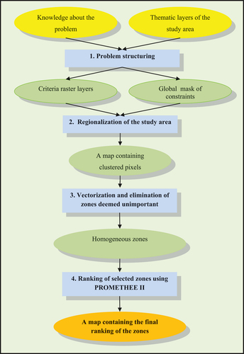
The approach we propose in this article (see Figure 1) applies to land use suitability analyzes carried out in areas whose representation requires the use of a large number of pixels. This approach includes four steps: (1) Problem structuring: at the end of which the raster layers of the various criteria as well as the raster of global constraints are created. (2) Grouping similar pixels in homogeneous zones by proceeding to the regionalization of the study area. (3) Vectorizing the resulting raster layer and eliminating zones that are smaller than what the intended use requires. Finally, (5) Ranking the selected zones, using PROMETHEE II, from the best to the worst. While the third step calls for simple procedures for someone who is used to work with GIS, steps 1, 2 and 4, on the other hand, need to be deepened.

Figure 1. Steps of the proposed approach for land-use suitability analysis.

2.1. Problem structuring

Using the different thematic layers that describe the study area (slope of the land, road network, hydraulic network, agglomerations, administrative divisions, types of land use, etc.) as well as knowledge gathered from experts and documents relevant to the problem addressed, this step leads to:

• Criteria identification, which is done in collaboration with the competent authorities and must lead to the definition of a clear list of the criteria that will be used in the evaluation of the various alternatives.

• Constraint definition, which are in relation to the intended land use that the alternatives must respect. Constraints such as: the slope of the land must be less than 20° are used to identify the zones that are likely to suit the needs of the desired site and to discard the other zones.

• Score calculation of the alternatives – each alternative being represented, initially, by a single pixel – on each criterion and creation of the raster associated with all the constraints. For each identified criterion, a series of operations, using GIS functions, is performed to obtain, on the one hand, a raster whose value associated with each pixel represents its performance with respect to this criterion and, on the other hand, a binary raster representing the associated constraint. The superposition of binary raster layers then makes it possible to define the zones which are suitable with respect to all the constraints and the zones to be discarded.

• Scores standardization: In the context of this article, the purpose of standardization is to make scores of the alternatives comparable across the different criteria which usually use different measurement units (metre, degree, hectare, kilometre, etc.). This step is necessary because the regionalization algorithm that is used is based on the calculation of a distance that involves the scores obtained at the level of each criterion. The linear transformation, which goes through the use of formula (1) when the performance of the alternatives (that is to say the values of gj()) are assumed to be maximized or formula (2) when the performances are assumed to be minimized, is the simplest form of normalization methods (Practical Gis, 2017).

(1) ${\mathbf{g}}_{\mathbf{j},\mathbf{norm}}\left(\mathbf{a}\right)\mathit{\hspace{0.17em}}=\mathit{\hspace{0.17em}}\mathit{\hspace{0.17em}}{\mathbf{g}}_{\mathbf{j}}\left(\mathbf{a}\right)-\mathbf{Mi}{\mathbf{n}}_{\mathbf{b}\mathit{\hspace{0.17em}}\in \mathbf{A}}\left({\mathbf{g}}_{\mathbf{j}}\left(\mathbf{b}\right)\mathit{\hspace{0.17em}}\right)/(\mathit{\hspace{0.17em}}\mathbf{Mi}{\mathbf{n}}_{\mathbf{b}\mathit{\hspace{0.17em}}\in \mathbf{A}}\left({\mathbf{g}}_{\mathbf{j}}\left(\mathbf{b}\right)\right)\text{break}-\mathit{\hspace{0.17em}}\mathbf{Mi}{\mathbf{n}}_{\mathbf{b}\mathit{\hspace{0.17em}}\in \mathbf{A}}\left({\mathbf{g}}_{\mathbf{j}}\left(\mathbf{b}\right)\right))$(1)

(2) ${\mathbf{g}}_{\mathbf{i},\mathbf{norm}}\left(\mathbf{a}\right)\mathit{\hspace{0.17em}}=\mathit{\hspace{0.17em}}\mathbf{1}-\mathit{\hspace{0.17em}}\left(\mathit{\hspace{0.17em}}{\mathbf{g}}_{\mathbf{j}}\left(\mathbf{a}\right)-\mathbf{Mi}{\mathbf{n}}_{\mathbf{b}\mathit{\hspace{0.17em}}\in \mathbf{A}}\left({\mathbf{g}}_{\mathbf{j}}\left(\mathbf{b}\right)\right)\mathit{\hspace{0.17em}}\right)\text{break}/\left(\mathit{\hspace{0.17em}}\mathbf{Mi}{\mathbf{n}}_{\mathbf{b}\mathit{\hspace{0.17em}}\in \mathbf{A}}\left({\mathbf{g}}_{\mathbf{j}}\left(\mathbf{b}\right)\right)-\mathit{\hspace{0.17em}}\mathbf{Mi}{\mathbf{n}}_{\mathbf{b}\mathit{\hspace{0.17em}}\in \mathbf{A}}\left({\mathbf{g}}_{\mathbf{j}}\left(\mathbf{b}\right)\right)\right)$(2)

where:

• A: is the set of all alternatives, a and b belong to A.

• g_j(a): is the performance of alternative a with respect to criterion j.

• g_j,norm(a): is the normalized performance of alternative a with respect to criterion j.

• Min_{b ϵA} (g_j(b)): is the minimum performance among all the alternatives with respect to criterion j.

• Max_{b ϵA} (g_j(b)): is the maximum performance among all the alternatives with respect to criterion j.

2.2. Regionalization of the study area

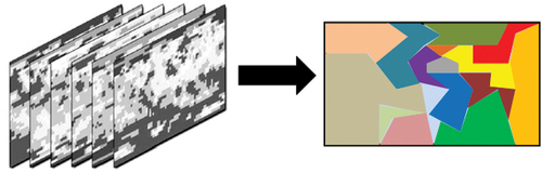
As we pointed out above, we propose, in this article, to use the technique of regionalization to form areas from pixels sharing similar properties. Starting from the observation that non-spatial multivariate clustering methods generally proceed to grouping objects that look alike without taking into account the constraint of spatial contiguity, the clusters formed from these methods contain elements that are not necessarily neighbours or contiguous in geographical space. Regionalization (see Figure 2) has then appeared to be a special form of non-spatial clustering that seeks to group neighbouring spatial objects to form zones while optimizing a similarity function (Miller and Han 2009).

Figure 2. Space regionalization.

Before addressing the details that are related to the choices that have been made at the level of our regionalization algorithm, we propose to make a horizontal reading of the principles that govern agglomerative hierarchical clustering approaches.

2.2.1. Non-spatial hierarchical clustering based on an agglomerative approach

According to Gan et al (2007), the final result of a hierarchical clustering algorithm, whether agglomerative or divisive, is a sequence of distinct groupings: C₀, C₁ … … C_n-1, with C₀ as being the weakest clustering (formed of n clusters, each cluster containing only one object) and C_n-1 as being the strongest clustering (a single cluster formed of n objects). These clusters are nested within each other because each cluster in C_k + 1 is either a cluster in C_k, or a cluster that results from the union of two or more clusters in C_k (Rohlf 1982).

In an agglomerative hierarchical clustering, each object is encapsulated in a cluster. At each iteration, the clusters that look the most alike, with respect to a certain measure of similarity, are merged until all the objects are grouped in the same cluster. Each time two clusters C_i, and C_j are merged, it is necessary to recalculate the distances that exist between the cluster resulting from this fusion and all the other clusters. According to Gan et al (2007), the choice of the proximity measure, which identifies the degree of similarity between two clusters, determines the hierarchical clustering method to be used. In the following paragraphs, we present properties of three hierarchical clustering methods, namely single-linkage clustering, full-linkage clustering and average-linkage clustering:

• Single-linkage clustering: This method uses the nearest neighbour distance to measure the degree of similarity between two clusters. According to Schlee et al (1975), this procedure often leads to the creation of clusters that are both long and sparse.

• Full-linkage Clustering: This method uses the distance of the farthest neighbour as a measure of similarity between clusters. According to Schlee (1975) this method generally produces clusters that are tight, hyper-spherical and discrete while having the characteristic of hardly joining with each other.

• Average-linkage Clustering: or ‘Unweighted peer group using the arithmetic mean’. This method proposes to see the degree of similarity as being the arithmetic mean of the distances calculated between all the peers of objects which constitute the clusters that one wishes to merge. According to Schlee et al (1975) this method aims to avoid the drawbacks of single-linkage and full-linkage clustering methods, namely, the formation of elongated clusters in the first case, or the formation of compact and tight clusters that leave aside the objects, which are hardly affiliated in the second case.

2.2.2. The proposed algorithm

The regionalization algorithm we proposed looks like this:

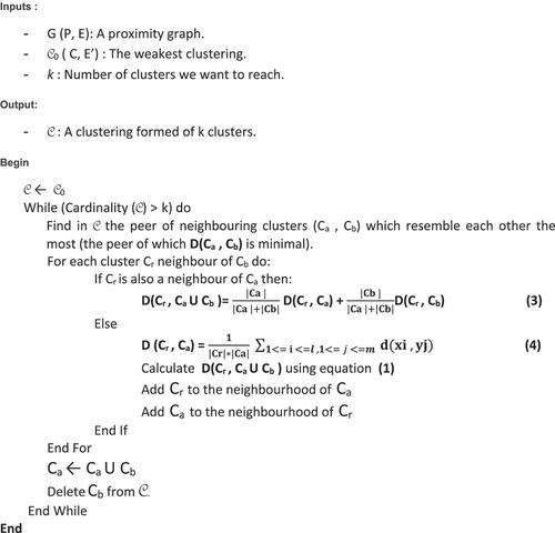
2.2.2.1. The regionalisation algorithm

In this algorithm, G(P,E) is a proximity graph. P is the set of vertices of this graph and E the set of edges connecting each peer of vertices. Each vertex x of P represents a pixel in the study area to which we associate a vector (x1, x2 … ,xd) of d values (d being the number of criteria that are taken into consideration in the grouping procedure). The neighbourhood of each vertex is automatically generated using the 4-neighbourhood of each pixel. In addition to being used to connect only neighbouring pixels, each edge e of E has a weight representing the degree of resemblance, between two vertices, x and y, using the Euclidean distance d (x,y). This distance is calculated as follows:

(3) $\mathbf{d}\mathit{\hspace{0.17em}}\left(\mathbf{x},\mathbf{y}\right)=\sqrt{{\sum }_{\mathbf{j}=1}^{\mathbf{d}}{\left(\mathbf{xj}-\mathbf{yj}\right)}^2}$(3)

C (C, E’) is another proximity graph where the vertices, C, are clusters containing, each, a certain number of pixels. E’ is the set of edges that connect each cluster with its neighbours. As in G, each edge of E’ is weighted using a distance D (like the nearest neighbour, the farthest neighbour, etc.) measuring the degree of resemblance between two clusters. Initially, since this clustering algorithm is based on an agglomerative approach, C represents the weakest clustering C ₀ in which each cluster C_i contains a single pixel. In the context of this article, we have chosen to use the Average_Linkage clustering to measure de degree of resemblance between two clusters (using equation (4)(4) $\mathrm{dj}\left(\mathrm{a},\mathrm{b}\right)=\mathrm{gj}\left(\mathrm{a}\right)-\mathrm{gj}\left(\mathrm{b}\right)$(4) ).

2.3. Ranking of the selected zones

This step is the last in the approach we propose (see Figure 1). Its objective is to rank the selected areas, using PROMETHEE II.

The objective of the PROMETHEE II method is to rank the alternatives from the best to the worst using a complete pre-order accepting situations of indifference and strict preference only. The preference structure, Pj, of PROMETHEE is based on pairwise comparisons where the deviation between the evaluations of two alternatives, a and b, on a particular criterion, j, is considered (Brans and De Smet 2016). Formally:

(4) $\mathrm{dj}\left(\mathrm{a},\mathrm{b}\right)=\mathrm{gj}\left(\mathrm{a}\right)-\mathrm{gj}\left(\mathrm{b}\right)$(4)

and

(5) $\mathrm{Pj}\left(\mathrm{a},\mathrm{b}\right)=\mathit{\hspace{0.17em}}\mathrm{Fj}\left(\mathrm{dj}\left(\mathrm{a},\mathrm{b}\right)\right)\mathrm{\forall }\mathit{\hspace{0.17em}}\mathrm{a},\mathit{\hspace{0.17em}}\mathrm{b}\mathit{\hspace{0.17em}}\in \mathit{\hspace{0.17em}}\mathrm{A}$(5)

Where:

• A: is the set of alternatives, a and b belong to A.

• j: is the criterion under consideration.

• gj(a): is performance of the alternative a on criterion j, we assume that the values of gj(a) are to be maximized.

• dj(a,b): is the difference between the performance of a and that of b with respect to criterion j.

• Pj: measures the degree of preference of a over b with respect to criterion j. Pj(a,b) ∈ [0, 1].

• Fj: the preference function. six types of preference functions are available. See (Brans and De Smet 2016) for more information on this subject.

In the case where Fj is of type V-shape with indifference, Pj takes the following form:

(6) $\mathrm{Pj}\left(\mathrm{dj}\left(\mathrm{a},\mathrm{b}\right)\right)=\left\{\begin{array}{c}0\mathit{if}\mathit{dj}\left(\mathit{a},\mathit{b}\right)<=\mathit{\hspace{0.17em}}\mathit{qj}\\ \frac{\mathrm{dj}\left(\mathrm{a},\mathrm{b}\right)-\mathrm{qj}}{\mathrm{pj}-\mathrm{qj}}\mathit{if}\mathit{qj}\mathit{\hspace{0.17em}}<\mathit{\hspace{0.17em}}\mathit{dj}\left(\mathit{a},\mathit{b}\right)\mathit{\hspace{0.17em}}<=\mathit{\hspace{0.17em}}\mathit{pj}\\ 1\mathit{if}\mathit{dj}\left(\mathit{a},\mathit{b}\right)\mathit{\hspace{0.17em}}>\mathit{\hspace{0.17em}}\mathit{pj}\end{array}\right.$(6)

Where:

• qj: or the indifference threshold, is the greatest difference in performance for which the situation of indifference is maintained between two alternatives on criterion j.

• pj: or the preference threshold, is the smallest difference in performance for which there is a situation of preference between two alternatives on criterion j.

In the following sections, we will present, in detail, the steps that must be followed to rank a certain number of alternatives.

2.3.1. Calculation of aggregated preference indices

For each pair of actions (a, b), an overall preference index, π (a,b), is calculated according to the deviation that there is in the evaluation of the alternatives on the different criteria on one hand and according to the weight of each criteria on the other hand. This index measures the degree of preference of action a over action b with respect to all the criteria. Formally:

(7) $\mathit{\pi }\mathit{\hspace{0.17em}}\left(\mathit{a},\mathit{b}\right)={\sum }_{\mathrm{j}=1}^{\mathrm{k}}\mathrm{Pj}\left(\mathrm{a},\mathrm{b}\right)\ast \mathrm{wj}$(7)

Where:

wj : represents the weight of relative importance given to criterion j.

A value of π (a,b) close to zero means that there is a low global preference of a over b, while a value close to 1 means that there is a high global preference of a over b.

2.3.2. Calculation of outranking flows

For each alternative, a, three outranking flows are calculated: positive outranking flow(ɸ⁺(a)), negative outranking flow(ɸ⁻(a)), and the net outranking flow(ɸ(a)). Details regarding the calculation of these three outranking can be found in Appendix A.

2.3.3. Ranking of alternatives

Once φ is calculated at each alternative, the pre-order is obtained by following the following rule (Brans and De Smet 2016):

$\left\{\begin{array}{c}\mathrm{a}\mathrm{Pb}\mathrm{iff}\mathit{\varphi }(\mathrm{a})>\mathit{\varphi }(\mathrm{b})\\ \mathrm{aIb}\mathrm{iff}\mathit{\varphi }(\mathit{a})=\mathit{\hspace{0.17em}}\mathit{\varphi }(\mathit{b})\end{array}\right.$

Where:

aPb: means a is preferred to b

aIb: a and b are indifferent

In this way, the net flow plays the same role as that of the utility function in establishing the final ranking.

3. Results

In the following paragraphs, we will present the results of a study focusing on the search for a landfill site using the approach we have proposed in this article. We begin by describing the context of this study. We then present the main results of the steps that constitute our approach as well as the final ranking of the obtained zones using PROMETHEE II.

3.1. Context of the study

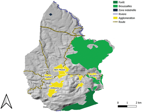
In developing countries, such as Algeria, landfills are the main outlet for most of the collected household waste. In most of the municipalities of Tlemcen, an Algerian department located in the far west of the country, the garbage collected is piled up in vacant lots which, for lack of resources, often end up being incinerated in the evening, thus creating significant health and environmental problems. The creation of a landfill site for household waste that will cover the needs of the department of Tlemcen is therefore more than necessary. We have chosen to look for the best site that will host the landfill at the level of the municipality of Béni mester because it occupies the centre of the department. This municipality covers an area of 6800 hectares, and has more than 20,000 inhabitants spread over 07 agglomerations (see Figure 3).

Figure 3. Municipality of Béni mester.

The choice of a landfill site is both a spatial and multi-criteria problem that can be described as difficult for several reasons: the visual aspect and the unpleasant odours that characterize landfills, liquids of percolation that emerge from them are considered to be a major source of pollution both for surface waters (rivers, dams, lakes, seas) and for groundwater, without forgetting the destruction of fauna and flora caused, first, by the creation of the site, then by the entry of the landfill into service. Several criteria must therefore be taken into consideration in order to ensure that the site, once set up, will have a very low impact on both the environment and the people who live in its vicinity.

3.2. Problem structuring

3.2.1. Criteria identification

Based on the work done in (Hiligsmann et al. 2006) and given the data that are available on the study area, we have chosen to work with the following criteria in searching for a site that will host the landfill:

3.2.1.1. Proximity to inhabited areas

In this criterion, we have included areas that are permanently inhabited (agglomerations) and any area that may be disturbed by the presence of a landfill (parks, leisure areas, military areas, industrial areas, forests, nature reserves, and tourist sites). A landfill must not be located at a distance of less than 100 m from these areas. This criterion should be maximized because the greater the distance separating the landfill from the areas concerned, the better the location of the site will be judged.

3.2.1.2. Proximity to the road network

To be easily accessible, a landfill should be as close to the road network as possible, however, the chosen site must not be located at a distance of less than 25 m from the road network. This criterion should be minimized.

3.2.1.3. Proximity to watercourses and bodies of water

To avoid any contamination of water by percolation liquids emanating from the landfill, the latter must be as far as possible from watercourses and bodies of water (natural lakes and artificial lakes that are upstream of water dams).

3.2.1.4. Land slope

A site is considered suitable if it is located on land with a slope of less than 18°. This criterion should be minimized.

3.2.1.5. Land acquisition cost

It depends on the value of the land which varies from one location to another. Once the potential sites have been identified, an expert estimates the value of each of them.

3.2.2. Constraint identification

Areas that are not suitable for the creation of a household waste landfill site are (Hiligsmann et al. 2006): flood-prone areas, areas that are below sea level, quarries (whether in operation or closed), areas which are on the catchment areas of groundwater, and areas near railways. To these areas, those which do not respect the constraints imposed by each criterion (such as areas whose slope is greater than 18°).

3.2.3. Calculation of the alternatives scores and production of the final constraint mask

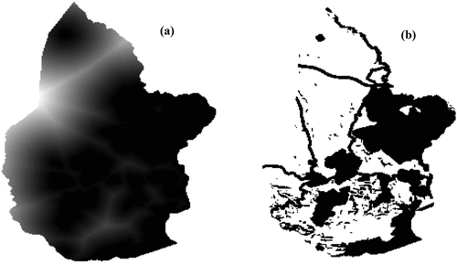
Using the free GIS software, QGIS, we calculated the pixel scores on each criterion and produced the final constraint mask. The analysis of the map of the final constraint mask allowed us to say that only 57.16% of the total area of the territory of the municipality can be qualified as suitable for hosting the landfill. Figure 4 illustrates on one side the map associated with the criterion: Proximity to agglomerations (a), on the other, the final constraint mask that was obtained (b).

Figure 4. Map of the criterion: proximity to agglomerations (a) and the final constraint mask(b).

3.3. Regionalization and vectorization of the study area

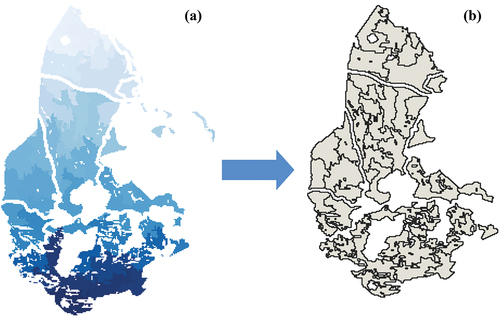
In Figure 5(a), we present the map that was generated by our regionalization algorithm. Initially containing 100 different groupings of pixels, this map then underwent a vectorization operation, followed by a filtering operation to eliminate zones whose area is less than 30 hectares. The vector layer that resulted from these two operations (Figure 5(b)) contains only 45 zones.

Figure 5. Regionalization (a) and vectorization (b) of the study area.

3.4. Ranking of the selected zones

In the last step of our approach, we propose to classify the zones that have emerged from the previous steps using the method: PROMETHEE II. By working with the criteria parameters of Table 1, the final ranking was obtained, with zones in dark blue occupying the first ranks (see Figure 6).

Figure 6. The final ranking of sites using PROMETHEE II.

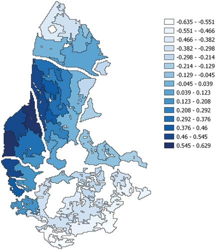
Table 1. Parameters associated with each criterion used in PROMETHEE II.

	Proximity to agglomerations	Proximity to road network	Proximity to watercourses	Land slope	Land acquisition cost
Q	400 m	500 m	1000 m	3°	2000 DA/m^2
P	800 m	1000 m	2000 m	6°	8000 DA/m^2
W	4	2	3	1	2
Preference Direction	Increasing	Decreasing	increasing	decreasing	decreasing

In table 01, the values of the parameters: w, q and p have been chosen as follows:

The values of the parameter w (representing the importance attributed to each criterion) have been chosen using a method called: The point allocation method (Odu 2019). The principle of this method is simple: The decision-maker has a certain number of points, he assigns to each criterion a number of points which is proportional to the importance he wishes to give to this criterion compared with the others, thus the criterion: Proximity to agglomerations is seen as being the most important criterion while the criterion: Land slope is considered to be the least important. In PROMETHEE, the sum of the weights of all the criteria is not necessarily equal to 1.

Concerning the parameters: q (representing the indifference threshold) and p (representing the preference threshold), it must be ensured that, at the level of each criterion, we have: q≤ p. The values of q that appear in table 01, have been chosen as follows:

• For the criteria which are described as being a distance (Proximity to agglomerations, Proximity to the road network and Proximity to watercourses), the values of q have been chosen to be proportional with the maximum distance which separates an alternative (a pixel) from an object that is of interest to us (agglomeration, river, road, etc.), so the greater this distance is at the level of a criterion, the greater the corresponding value of q.

• For the criterion: Land slope, all the pixels whose slope is greater than 18° have been excluded from the study. For those who remain, 3° seemed to be correct to us as a threshold of indifference.

• For the last criterion, namely: Land acquisition cost, and according to our point of view, the value of 2000 DA seemed good to us for q.

For all the criteria that were considered in this study, with the exception of the last one, we chose p = 2*q.

4. Discussion and conclusions

In this article, we have proposed a decision-making approach to analyse the suitability of an area for a particular use. The proposed approach is based on four steps that involve:

• A GIS: whose main role is to generate the maps associated with the different criteria, the global mask of the constraints which are associated with the intended use, while going through the use of the data conversion functions from raster format to vector format as well as filtering functions.

• A regionalization algorithm: to form a set of homogeneous areas from neighbouring pixels having similar performances on the different criteria.

• PROMETHEE II, a multi-criteria decision support method, a method whose role is to classify the zones obtained, by applying the regionalization algorithm, from the best to the worst.

The proposed approach was successfully applied in a study focusing on the search for a site intended to host a landfill.

We present, in Figure 7, the result of the final classification of the pixels which constitute the study area using the WLC method. Thanks to the ease of its implementation, the results of this method have always been compared with those of studies that have been made as part of a land use suitability analysis using new approaches. WLC was applied using the same weighting coefficients, but in the normalized version such that the sum of the coefficients is 1, as those used in our approach.

Figure 7. Final ranking of pixels using the WLC method.

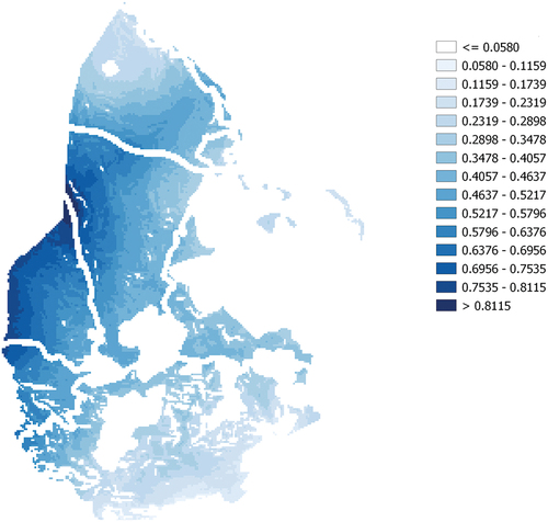
For the comparison of the results to make sense, we chose to classify the pixels using the same number of equivalence classes as that of our study, namely 15. By comparing Figures 6 and 7, we can easily see that the classification of the zones is in line with that of the pixels, in other words, the best sites, as indicated by the classification of the zones which was obtained with PROMETHEE II, are located where there are groupings of pixels whose suitability index is large, as indicated by the ranking that was obtained with WLC.

In our approach, the municipality of Tlemcen was divided into a certain number of potential sites whose borders were clearly defined, then, using PROMETHEE II, each site was assigned to a rank. Our result is therefore clearer than the one obtained using the WLC method, which simply calculates an overall score at the level of each pixel.

The need to compare each alternative with all the others prevents the use of outranking methods in the context of a land use suitability analysis because the study area is often represented by an important number of pixels and each pixel is considered as an alternative. We therefore proposed to regionalize the studied area by grouping neighbouring pixels with similar properties into zones. This way of seeing things has the following advantages:

• Automatic generation of potential alternatives that may be suitable for the intended use. Unlike the approaches proposed in (Joerin, Thériault, and Musy 2001, Marinoni 2006, Chakhar and Mousseau 2008), which either rely on heuristics that are not based on solid theoretical foundations as in (Marinoni 2006, Chakhar and Mousseau 2008) or are not completely well defined as in (Joerin, Thériault, and Musy 2001), the formation of zones, in our case, relies on the adaptation of an agglomerative hierarchical clustering algorithm whose theoretical foundations are well known.

• Following the tracks of Malczewski and Rinner (2015), Malczewski and Jankowski (2020), the use of the regionalization algorithm places us in the perspective of a GIS-MCDA approach that can be described as spatially explicit because the formation of the homogeneous zones is based on the exploitation of the variation of the performances of the pixels on the different criteria through the space, in addition, the use of the average of the Euclidean distances, also known as: Average-Linkage Clustering, as a similarity distance between clusters enables us to obtain zones whose shapes have characteristics which are known in advance.

• The proposed regionalization algorithm gives full control over the number of zones one wishes to form, which subsequently allows one to use an outranking method to rank the different alternatives from best to worst, or assign them to a predefined set of categories etc.

It must be said that there are no problems with the formation of zones when the size of the studied area is relatively small, as was the case in the study conducted within the context of this article, but the larger the study area, the longer the response times become. To optimize response times, we propose to form a Minimal Spanning Tree (MST), which for n vertices requires only n-1 edges to connect them and whose sum of edge weights is minimal, from the initial proximity graph, then apply the regionalization algorithm to the MST to form the requested zones.

Disclosure statement

No potential conflict of interest was reported by the author(s).

Appendix A

Calculation of outranking flows

For each action a, a three quantities are calculated. These quantities refer to positive outranking flow, negative outranking flow and net outranking flow.

Positive outranking flow

Positive outranking flow, or ɸ+(a), represents the power of action a, it measures the degree to which a outranks all other alternatives.

${\varphi }^{+}\left(\mathit{a}\right)\mathit{\hspace{0.17em}}=\frac{1}{\mathrm{n}-1}\sum _{\mathrm{x}\in \mathrm{A}}^{\mathit{\hspace{0.17em}}}\mathit{\pi }\left(\mathrm{a},\mathrm{x}\right)\mathit{\hspace{0.17em}}$

Negative outranking flow

Negative outranking flow, or ɸ-(a), represents the weakness of action a, it measures the degree of outranking of action a by the other actions.

${\varphi }^{-}\left(\mathit{a}\right)\mathit{\hspace{0.17em}}=\frac{1}{\mathit{n}-1}\sum _{\mathit{x}\in \mathit{A}}^{\mathit{\hspace{0.17em}}}\mathit{\pi }\left(\mathrm{x},\mathrm{a}\right)\mathit{\hspace{0.17em}}$

Net outranking flow

Net outranking flow, or ɸ (a), represents the difference between the positive and the negative flows. The higher the net flow, the better the alternative.

$\mathit{\varphi }\left(\mathrm{a}\right)={\varphi }^{+}\left(\mathrm{a}\right)+{\varphi }^{-}\left(\mathrm{a}\right)$

Where:

$\left\{\begin{array}{c}-1<=\mathit{\hspace{0.17em}}\mathit{\varphi }(\mathit{a})<=1\\ \sum _{\mathrm{a}\in \mathrm{A}}\mathit{\phi }\left(\mathrm{a}\right)=0\end{array}\right.$

References

- Bagherzadeh, A., and A. Gholizadeh. 2016. “Modeling Land Suitability Evaluation for Wheat Production by Parametric and TOPSIS Approaches Using GIS, Northeast of Iran.” Modeling Earth Systems and Environment 2 (3): 1–11. https://doi.org/10.1007/s40808-016-0177-8.
- Brans, J. P., and Y. De Smet. 2016. “PROMETHEE Methods.” In Multiple Criteria Decision Analysis: State Of The Art, edited by S. Greco, M. Ehrgott, and José R. Figueira, 187–219. New York, NY: Springer.
- Chakhar, S., and V. Mousseau. 2008. “GIS‐Based Multicriteria Spatial Modeling Generic Framework.” International Journal of Geographical Information Science 22 (11–12): 1159–1196. https://doi.org/10.1080/13658810801949827.
- Dehghan, P., H. Azarnivand, H. Khosravi, G. Zehtabian, and A. Moghaddamnia. 2021. “An ecological agricultural model using fuzzy AHP and PROMETHEE II approach.” Desert 26 (1): 71–83.
- Demesouka, O. E., A. P. Vavatsikos, and K. P. Anagnostopoulos. 2013. “Suitability Analysis for Siting MSW Landfills and Its Multicriteria Spatial Decision Support System: Method, Implementation and Case Study.” Waste Management 33 (5): 1190–1206. https://doi.org/10.1016/j.wasman.2013.01.030.
- Gan, G., C. Ma, and J. Wu. 2007. Data Clustering: Theory, Algorithms, and Applications. Pyladelphia, Pennsylvania: Society for Industrial and Applied Mathematics.
- Gbanie, S. P., P. B. Tengbe, J. S. Momoh, J. Medo, and V. T. S. Kabba. 2013. “Modelling Landfill Location Using Geographic Information Systems (GIS) and Multi-Criteria Decision Analysis (MCDA): Case Study Bo, Southern Sierra Leone.” Applied Geography 36:3–12. https://doi.org/10.1016/j.apgeog.2012.06.013.
- Hiligsmann, S., M. Lardinois, S. I. Diabaté, and P. Thonart. 2006. Guide pratique sur la gestion des déchets ménagers et des sites d’enfouissement technique dans les pays du Sud. Québec, Canada: Institut de l’Energie et de l’Environnement de la Francophonie (IEPF).
- Joerin, F., M. Thériault, and A. Musy. 2001. “Using GIS and Outranking Multicriteria Analysis for Land-Use Suitability Assessment.” International Journal of Geographical Information Science 15 (2): 153–174. https://doi.org/10.1080/13658810051030487.
- Ligmann-Zielinska, A., and P. Jankowski. 2012. “Impact of Proximity-Adjusted Preferences on Rank-Order Stability in Geographical Multicriteria Decision Analysis.” Journal of Geographical Systems 14 (2): 167–187. https://doi.org/10.1007/s10109-010-0140-6.
- Malczewski, J. 2011. “Local Weighted Linear Combination.” Transactions in GIS 15 (4): 439–455. https://doi.org/10.1111/j.1467-9671.2011.01275.x.
- Malczewski, J., and P. Jankowski. 2020. “Emerging Trends and Research Frontiers in Spatial Multicriteria Analysis.” International Journal of Geographical Information Science 34 (7): 1257–1282. https://doi.org/10.1080/13658816.2020.1712403.
- Malczewski, J., and X. Liu. 2014. “Local Ordered Weighted Averaging in GIS-Based Multicriteria Analysis.” Annals of GIS 20 (2): 117–129. https://doi.org/10.1080/19475683.2014.904439.
- Malczewski, J., and C. Rinner. 2015. Multicriteria Decision Analysis in Geographic Information Science. New York: Springer.
- Marinoni, O. 2006. “A Discussion on the Computational Limitations of Outranking Methods for Land-Use Suitability Assessment.” International Journal of Geographical Information Science 20 (1): 69–87. https://doi.org/10.1080/13658810500287040.
- Mena, S. B. 2000. “Introduction aux méthodes multicritères d’aide à la décision.” Biotechnology, Agronomy, Society and Environment 4 (2): 83–93.
- Miller, H. J., and J. Han. 2009. Geographic Data Mining and Knowledge Discovery. New York: CRC press.
- Odu, G. O. 2019. “Weighting Methods for Multi-Criteria Decision Making Technique.” Journal of Applied Sciences and Environmental Management 23 (8): 1449–1457. https://doi.org/10.4314/jasem.v23i8.7.
- Rohlf, F. J. 1982. 12 Single-link clustering algorithms. Handbook of Statistics 2:267–284. https://doi.org/10.1016/S0169-7161(82)02015-X.
- Romano, G., P. Dal Sasso, G. T. Liuzzi, and F. Gentile. 2015. “Multi-Criteria Decision Analysis for Land Suitability Mapping in a Rural Area of Southern Italy.” Land Use Policy 48:131–143. https://doi.org/10.1016/j.landusepol.2015.05.013.
- Roy, B., and D. Bouyssou. 1993. Aide multicritère à la décision: méthodes et cas. Paris: Economica.
- Schlee, D., P. H. A. Sneath, R. R. Sokal, and W. H. Freeman. 1975. “Numerical Taxonomy. The Principles and Practice of Numerical Classification.” Systematic Zoology 24 (2): 263. https://doi.org/10.2307/2412767.
- Sotiropoulou, K. F., and A. P. Vavatsikos. 2021. “Onshore Wind Farms GIS-Assisted Suitability Analysis Using PROMETHEE II.” Energy Policy 158:112531. https://doi.org/10.1016/j.enpol.2021.112531.
- Vavatsikos, A. P., O. E. Demesouka, and K. P. Anagnostopoulos. 2020. “GIS-Based Suitability Analysis Using Fuzzy PROMETHEE.” Journal of Environmental Planning and Management 63 (4): 604–628. https://doi.org/10.1080/09640568.2019.1599830.
- Vavatsikos, A. P., K. F. Sotiropoulou, and V. Tzingizis. 2022. “GIS-Assisted Suitability Analysis Combining PROMETHEE II, Analytic Hierarchy Process and Inverse Distance Weighting.” Operational Research 22 (5): 5983–6006. https://doi.org/10.1007/s12351-022-00706-0.