Spatial heterogeneity in the urban household living conditions: A-GIS-based spatial analysis

ABSTRACT

The unplanned urban expansion and extreme population pressure have caused several bottlenecks for city dwellers, which have been reflected in the form of inter-urban spatial inequality in living conditions at the household level. The present study integrates GIS with a composite synthetic index to measure the spatial variation of urban household conditions across 146 urban centers in Eastern India (West Bengal). The study critically scrutinizes the influence of urban housing conditions, amenities level, and asset possession on the well-being of urban households. Based on these three inter-connected dimensions, a composite index for urban household living condition index was computed based on the optimum combinational composite index model (OCCIM). Besides, the study provides insight into the geographic distribution of urban household living conditions considering their spatial patterns, hot spots, and clusters identification. The spatial heterogeneity of the selected dimensions is shown on the maps produced using the GIS. The spatial variation was measured using Moran’s I at the global level and Getis-Ord Gi * to identify influential locations through clusters and hot spots detection of urban housing condition, amenities level, assets possession, and composite living condition scenario. Additionally, the constructed UHdCLI model’s consistency is assessed using the r-squared value of regression analysis (R² = 0.815). The latest findings provide a realistic view of the spatial inter-urban variations that exist at the level of particular households concerning several aspects of their standard of life.

KEYWORDS:

• Urban
• GIS
• spatial analysis
• inequality
• hotspot

1. Introduction

In the midst of the 1960s, there was a necessity for assessing the quality of living in urban households through an endeavour to ameliorate the situation of the poor and disadvantaged population (Das and Mistri 2013; Vitale 2008; Wilson 2012). For quite a long time, GDP was the only measure of growth and prosperity in terms of material possessions (Behera 2016; Giannetti et al. 2015; Jackson 2013; Weiss 2007). However, gross domestic product (GDP) or economic performance alone cannot accurately portray the actual dimensions of people’s quality of living in urban households (Diener and Tov 2012). The notion of living quality is employed in many different disciplines, from philosophy and social sciences to politics and environmental studies and sometimes even health sciences (Gatersleben and Vlek 1998; Haas 1999; Mondal 2020). In common use, it denotes the state of affairs in which people, families, and communities as a whole are healthy and happy (Leaver et al. 2007; Massam 2002; Newman and Schnare 1997). Well-being, contentment, and happiness are all closely linked concepts that may be difficult to comprehend. Access to basic amenities is a critical component of economic progress, and improving infrastructure is crucial to ensuring that everyone benefits from that growth, but it is not the only indicator of people’s quality of living (Deller et al. 2001; Shaffer, Deller, and Marcouiller 2006; Visvizi et al. 2018). Social scientists and geographers are constantly expanding the list of indicators that may be used to judge the quality of living in different spatial units. This research has expanded our knowledge of the factors determining the quality of living, including the availability of amenities, assets, and adequate accommodation.

The large spectrum in housing quality directly reflects the country’s diverse socioeconomic strata and has significant implications for the quality of living in individual households (Ahluwalia 2019; Sengupta, Shaw, and Kundu 2022). The demographic shifts, economic growth, rise in the number of nuclear households, and spread of urbanization that have occurred in India over the last decade have all contributed to the rapid expansion of the country’s housing market (Ministry of Housing & Urban Poverty Alleviation 2012). Overcrowded slums sit alongside high-rise residential buildings housing small dwellings of varying sizes (Agarwal et al. 2021). The rising cost of land and building materials in overcrowded cities has made India’s urban housing crisis all the more apparent (D’souza 2019; Ghosh and Bandyopadhyay 2019). The need to provide enough housing and other social infrastructure, especially in major urban centres that have drawn new businesses and services, has grown imperative (D’souza 2019; Ghosh and Bandyopadhyay 2019; Patel, Shah, and Beauregard 2020). According to a recent report, India would likely need 25 million more affordable dwellings by 2030 to accommodate the country’s expanding urban population. Therefore, monitoring and understanding the issue of household quality of life is, thus, of paramount importance.

Well over half of the world’s population currently resides in urban areas, and as a result, urbanization has become the primary focus of contemporary urban geographies in developing nations (Bose and Chowdhury 2020; Henderson and Turner 2020; Kang et al. 2020; Roy et al. 2021). The migration from the countryside to the city has altered people’s routines, habits, and social structures (Charlier 2020; Prieto Curiel et al. 2018). One of West Bengal’s distinguishing qualities is its urban nature. Urbanization in West Bengal is both vibrant and complex because of the state’s wealth of natural resources, its history of rapid urbanization, and the way its high population density has given birth to a rich rural traditional background (Das and Das 2019; Onda et al. 2019; Sarkar 2019).

GIS has significantly assisted in the handling, processing, visualizing, and analysing spatial data (de Moura and Procopiuck 2020). It might be a handy tool for urban and regional planning when integrated with spatial statistical models (Roy et al. 2022). Several studies have used GIS as an effective tool to identify the potential results and modelled urban social elements at the spatial level (Dadashpoor, Rostami, and Alizadeh 2016; de Moura and Procopiuck 2020; Gopal et al. 2009; Kuai and Zhao 2017; Maryada and Thatiparthi 2020). The optimum application of GIS and statistical models simultaneously assisted in determining the zone of potential bottleneck with high risk and challenges and the geographic space with better performance compared to the other areas (Haque 2016; Mondal and Das 2022). In that sense, the study demonstrates how GIS can effectively map the spatial nature of social-economic status and the associated living conditions of urban households in the different urban centres in West Bengal.

A limited number of research endeavours exist to evaluate the spatial disparity in urban domiciliary living circumstances and associated factors. Osumanu et al. (2016) scrutinized the housing conditions within the Wa Municipality of Ghana, revealing inadequate infrastructure and precarious living situations. This study underscores the urgency for innovative approaches to regulate the housing sector and prioritize essential services for egalitarian urban development. Mboumboue and Njomo (2016) explore the correlation between renewable resources and living conditions in rural households, explicitly focusing on Cameroon. They accentuate this country’s substantial solar, biomass, and hydroelectric potentials while advocating for an escalation in renewable resource utilization alongside integrating sustainable development principles into policies. Furthermore, Liu et al. (2017) examine the emergence of female headship in Latin America and its connection to evolving household arrangements. Das and Mistri (2013) assess dwelling quality at a household level based on Census data from Indian states. The southern and western states exhibit positive dwelling quality, whereas their eastern and north-eastern counterparts possess substandard quality dwellings. A composite index employing Principal Component Analysis is employed to calculate dwelling quality. Das et al. (2021) evaluate household living conditions and disparities within India’s Bundelkhand region using Composite Index and other indices. The outcomes indicate noteworthy discrepancies across districts, which necessitate authorities’ focus on enforcing existing policies whilst formulating effective strategies to ameliorate living conditions within this locale. Zou and Luo (2019), meanwhile, analyse energy consumption disparities amongst rural households in China; they discovered that factors such as health condition of household heads, educational attainment levels, off-farm employment status, size of households, as well as economic situation exert influence over patterns of energy consumption. Ruiz-Tagle and Urria (2022), examines how overcrowding affects mental health in Chilean households, revealing a correlation between increased overcrowding and heightened levels of mental issues. Furthermore, Majumder et al. (2023) recently quantified the social vulnerability at a household level within urban areas of Eastern India by considering exposure, sensitivity, and adaptive capacity. The findings indicate high levels of urban social vulnerability, which accentuate the urgency for targeted strategies to address the predicaments residents of urban households face. These studies mentioned above have neglected to assess spatial heterogeneity in urban household living conditions. Existing methodologies have often focussed solely on specific aspects of living conditions or relied upon qualitative assessments without capturing a comprehensive overview. Moreover, these studies have not incorporated GIS with composite synthetic indices, limiting spatial analysis possibilities. Additionally, an all-encompassing framework that collectively encompasses housing conditions, amenity levels, and asset possession has been lacking, thus impeding holistic comprehension regarding urban household living circumstances. Thus, our research endeavours to fill these gaps by providing an innovative and robust framework. By integrating GIS alongside a composite synthetic index while employing the OCCIM model, our study offers a comprehensive and quantitative approach towards measuring and analyzing spatial heterogeneity pertaining to urban household living conditions.

This present research evaluates the quality of living in households based on three factors: housing conditions, access to basic amenities, and asset ownership. In order to spot economic and affordability gaps across urban areas, it is essential to understand the status of the housing conditions (Nijman and Wei 2020; Zhang 2020). Keeping tabs on the state of household amenities like water and electricity sends a message to the administration about the need to address the disparities and delays in distributing these services across various urban spatial units (Ahmed and Khan 2018; Karlsson et al. 2020). It is easy to gauge urban households’ living standards and financial well-being because of readily accessible asset possessions (Ansary and Das 2018; Guin and Das 2015a). Therefore, the current research used these three factors to compute a composite synthetic index and to compare the spatiality of the household living conditions in 146 urban areas of Eastern India (West Bengal). The present research is novel because there is limited work regarding the spatial variations of urban household living conditions with the use of GIS considered before. This research aims to identify the geographic distributional pattern and to map out how various urban centres spatially vary in terms of household quality of living. The significance of studying the spatial aspects of quality of living cannot be overstated since it allows planners to pinpoint geographically disadvantaged places (Garau and Pavan 2018; Liu et al. 2018). The geographic growth pattern is profoundly influenced by the proximity of additional urban centres to each other (Cottineau et al. 2019; Ran et al. 2021; Salem et al. 2021). Although the population parameter and location factor plays an essential part in defining the quality of services supplied by those urban centres, they are all helped by the clustering effects when they are close to one another (Cottineau et al. 2019; Moretti 2021). As a result, the provision of essential services and the growth of supporting infrastructure are greatly aided by clustering urban centres (Fotheringham and Sachdeva 2022). Under these conceptual conditions, it is fascinating to investigate the household quality of living in different urban areas of West Bengal, and this approach can be further applied to other parts of the world’s urban centres.

Thus, constructing upon the discussion above, this study pursued three primary objectives to address the research problem comprehensively: i) To investigate the geographical variability of urban household housing conditions, acces to amenities, and asset possession level in the study area. ii) To examine the spatial distribution of household multidimensional living conditions in urban areas of West Bengal using GIS-based spatial analysis. Iii) To identify patterns of spatial heterogeneity in urban household living conditions and explore their underlying causes by implementing exploratory spatial data analysis techniques. We have some broad research questions to simplify the analysis based on the constructed objectives. These research questions are as follows: i) How do household living conditions vary across different spatial locations within urban areas in the study area? ii) How can GIS-based spatial analysis techniques help understand and visualize spatial heterogeneity patterns in urban household living conditions? iii) Are specific household indicators significantly influencing the disparities in urban living conditions? iv) What policy interventions can be proposed to mitigate the disparities in household living conditions and promote equitable urban development?

2. Materials and methodology

2.1. Study area

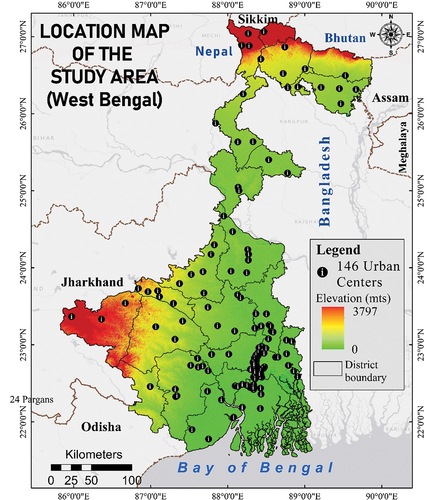
In the present study, 146 urban centres from Eastern India (West Bengal), which were distributed over 23 districts, were considered (Figure 1). According to the Indian census, a town or city is classified as an urban area if it has a municipality, corporation, cantonment board, or notified town area committee (Yadav, Rajak, and Yadav 2021). However, the present research region is the Eastern part of the Indian state known as West Bengal or ‘Paschim Banga’, which spans the coordinates 21°20’N to 27°32’N and 85°50’E to 89°52’E. Part of the Chhotanagpur plateau to the west and the lower Ganga plain to the east are also included in its expansive reach, which begins at the foot of the Darjeeling Himalayas and finishes at the Bay of Bengal in the south (Sarkar 2019). A total of 91.3 million people resided in the state as of the 2011 Census, and its 88,752 km² area comprised 2.7% of the total land area of the nation. According to the 2011 Census, the population density was 1,028 people per square kilometre, much higher than the national average of 382 (Kumar et al. 2020). The entire state’s administrative structure was split up into the following five regions: (i) Mountainous region (Darjeeling district), (ii) Northern Plain region (Jalpaiguri, Koch Bihar, Uttar Dinajpur, Dakshin Dinajpur, and Malda districts), (iii) Southern Plain region (Murshidabad, Birbhum, Barddhaman, Nadia, Hugli, Howrah, North 24 Parganas, and Kolkata districts), (iv) Plateau region (Purulia, Bankura and Paschim Medinipur districts) and (v) Coastal Plain region (South 24 Parganas and Purba Medinipur districts) (Bhattacharjee and Behera 2018). Besides the formation of Alipurduar district in 2014, Kalimpong district in 2017, Jhargram district in 2017, and the division of Bardhaman district into Purba and Paschim Bardhaman district, West Bengal now has a total of 23 districts. Therefore, the present research looked at the spatial distribution of the urban household quality of living across the urban centres (including municipalities, notified area, industrial townships) distributed over 23 districts of West Bengal.

Figure 1. Location map of the study area. The map showing the selected 146 urban centres, districts boundary and relief.

2.2. Data source, collection, and its processing

For the current study, the critical indicators relating to urban households were collected from the Socio-Economic Caste Census (SECC), which is administered by the Ministry of Housing and Urban Poverty Alleviation (MoHUPA) under the Government of India. The SECC serves as a valuable data source and can be accessed at the official website https://secc.gov.in/homePageUrban.htm. The SECC-2011 survey using the respondent-based canvasser method, which has been chosen as the preferred approach for data collection. It worth mentioning that, to ensure the quality of data, the surveyors will be thoroughly trained on the survey objectives, methodology, and ethical considerations. The results of the SECC-2011 survey were made publicly available in 2015 which further updated in 2016, providing researchers and policymakers with easy access to a rich source of urban household data.

More specifically for study, the data was acquired for three major components from the urban household interface, i.e. housing/dwelling, amenities, and asset possession (Table 1). From the housing components, the data were collected for variables, namely predominant wall materials (WA), predominant material of roof (RF), ownership status (OS), and dwelling room status, which includes no room (NR), one room (OR), and more than one room (MOR). From the amenities section, six types of household amenities data were collected, i.e. availability of drinking water (W), source of electricity that includes no electricity (NE) and Electricity availability (EL), water-seal latrine facility (LT) exclusively for the household, household having no waste water-outlet (NWO) connections, and exclusive kitchen availability (KT) for the respective urban centres of the study area. Lastly, for assets possession, Refrigerator Availability (RF), no communications (NCM) that includes no telephone and mobiles, Computer/Laptop Availability (CL), no motorize wheelers availability (NW), air conditioner (ac) availability, and availability of washing machine (WM). All the data were acquired in.xlsx format; subsequently, all these collected data were then rearranged, cleaned, and regenerated using a different variable per the study’s need. To ensure compatibility with a GIS environment and facilitate the analysis, the data underwent a thorough cleaning and processing stage. By cleaning and processing the data to meet GIS compatibility requirements and using appropriate methods, the dataset is optimized for spatial analysis. For the present research, Google Earth was used to acquire point data for the urban centres, and ESRI-based ArcGIS was used for mapping and visualization purposes. Besides, Jamovi software is used for data processing and statistical analysis. Figure 2 represents the overall methodology for the present study.

Figure 2. Methodological flowchart adopted for the present study.

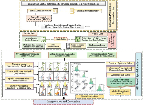
Table 1. Selected dimensions, indicators, and variables for the assessment of Urban Household Condition of Living.

Index	Indicators	Variables Description	Symbol	Relation
Housing Quality Index	House Material	Household Having Houses With Predominant Material Of Wall In Durable Nature	Wall	+
		Household Having Houses With Predominant Material Of Roof In Durable Nature	Roof	+
	Ownership	Household Having Own House	Ownership	+
	Dwelling Room Status	Household Having No Dwelling Room	No Room	-
		Household Having One Dwelling Room	One Room	-
		Household Having More Than One Dwelling Room	More Room	+
Household Amenities Index	Drinking Water	Household Having Availability Of Drinking Water Sources Within The Premises	Drinking Water	+
	Kitchen	Household Having Exclusive Kitchen Availability	Kitchen	+
	Lighting Source	Household Having No Sources Of Lighting	No Light	-
		Household Having Electricity As Main Sources Of Lighting	Electricity	+
	Sanitation	Household Having No Waste Water-Outlet Connections	No Waste Outlet	-
		Household Having Water-Seal Latrine Exclusively For The Household Members	Latrine	+
Household Assets Possession Index	Basic and essential assets	Households Having Refrigerator Availability	Refrigerator	+
		Household Having No Modern Communication Facilities	No Communication	-
		Household Having Computer/Laptop Availability	Computer	+
		Household Having No Motorize Wheelers Availability	No Wheelers	-
		Household Having Air Conditioner (AC) Availability	Air Conditioner	+
		Household Having Washing Machine Availability	Washing Machine	+

2.3. Measuring the household living conditions and heterogeneity in the urban centers

Various households living conditions methods are available for urban areas. For instance, works done by Haque (2016) to access the city-level infrastructure and basic amenities level based on assets, recreational facilities, attitude, and physical infrastructure as a collective umbrella of urban area development. Apparently, several factors influence and strengthen household well-being (Guin and Das 2015b; Guin 2016; Hosseini et al. 2021). Rapid population expansion, escalating costs of living, and the prime commercial role in the economy render urban space extremely important for policymakers. It is a space where lots of people are forced to survive with low wealth, minimum asset possessions and dilapidated housing conditions.

Therefore, for the present study, we mainly focus on measuring the household living conditions and associated patterns of spatial heterogeneity in the urban centres of west Bengal based on three major interacting dimensions (Table 1). The inequality context is clearly emphasized, and living condition status is determined using a synthetic index construction approach. Moreover, household quality of living assessment focuses on the household’s capacity to resist and promptly recover losses, engaging more in wealth generation (Biswas and Banu 2021; Haque 2016; Sharma and Chandrasekhar 2014). The study was categorically measuring the urban household condition of living index (UHdCLI) based on the composite assessment method three sub-index, i.e. Urban Housing Condition Index (UHgCI), Urban Household Amenities (UHdAMI), and Urban Household Assets Possession (UHdAPI) specifically as follows.

(1) $\mathrm{UHdCLI}=\mathrm{f}\left(\mathrm{UHgCI},\mathrm{UHdAMI},\mathrm{UHdAPI}\right)$(1)

In addition to choosing the technique of household living conditions, it is also essential to choose the appropriate indicators, as it should influence the rationality, efficiency, and validity of the household living condition assessment. In this study, the indicator set was chosen based on the availability of datasets, how well they fit with local settings, and their importance in accommodating the development strategies of the study area.

2.4. Normalization of indicators

The indicators will be normalized in order to assure overall comparability. The normalization was performed using the technique developed for calculating the Human Development Index (UNDP 2006). Subsequently, to generate adjusted values, the employed indicators are normalized so that they all fall between 0 and 1 (Majumder 2021; Majumder et al. 2022). The study utilized positive and negative indicators that need to be adjusted with different equations. If the indicators are assumed to be a positive relationship with household status, the formula will be described below.

(2) ${\mathrm{Z}}_{\mathrm{ij}}=\frac{{\mathrm{X}}_{\mathrm{ij}}-\mathrm{Min}\left({\mathrm{X}}_{\mathrm{ij}}\right)}{\mathrm{Max}\left({\mathrm{X}}_{\mathrm{ij}}\right)-\mathrm{Min}\left({\mathrm{X}}_{\mathrm{ij}}\right)}\left(\mathrm{for}{\mathrm{X}}_{\mathrm{ij}}\mathrm{being}\mathrm{a}\mathrm{positive}\mathrm{relation}\uparrow \right)$(2)

However, if the indicators are assumed to be negative relationship with household wellbeing, the above formula will be changed as of following,

(3) ${\mathrm{Z}}_{\mathrm{ij}}=\frac{\mathrm{Max}\left({\mathrm{X}}_{\mathrm{ij}}\right)-{\mathrm{X}}_{\mathrm{ij}}}{\mathrm{Max}\left({\mathrm{X}}_{\mathrm{ij}}\right)-\mathrm{Min}\left({\mathrm{X}}_{\mathrm{ij}}\right)}\left(\mathrm{for}{\mathrm{X}}_{\mathrm{ij}}\mathrm{being}\mathrm{a}\mathrm{negative}\mathrm{relation}\downarrow \right)$(3)

Where, Zij is the normalized value of jth indicator for urban unit i. Xij is the unadjusted value of jth indicator for urban unit i. lastly, the Max (Xij) and Min (Xij) is the maximum and minimum unadjusted value of jth indicator for urban unit i, respectively.

2.5. Construction of synthetic indexes for urban household living conditions

A large number of indicators input can determine the considered UHdCLI. Therefore, to measure the status of urban household living condition for a particular urban centre, 18 indicators have been categorized under three sub-dimensional indexes (each dimension include six indicators) instead of any single dimension. Subsequently, once the normalized scores have been computed for entire selected indicators using the ‘Optimum Combinational Composite Index Method’ (OCCIM) of Halder (2019), Narain et al. (1991) to construct sub-indexes (Di) of UHdCLI by adding all normalized scores, the Di can be obtained as follows:

(4) ${\mathrm{D}}_{\mathrm{i}}=\frac{{\mathrm{C}}_{\mathrm{i}}}{\mathrm{C}}$(4)

Here, the Di represent the development of three dimensional index i.e. UHgCI, UHdAI, and UHdAPI of i^th urban centre. The closer Di is to 0 the more developed is the state, and the closer to unity, the less developed the state. Ci is the pattern of development in indicators of the employed sub-indexes,

(5) $\text{C}=\overline{C}+3\mathit{\sigma }{\text{C}}_{\text{i}}$(5)

(6) $\overline{C}=\frac{{\displaystyle \sum _{\text{i}=1}^{\text{N}}{\text{C}}_{\text{i}}}}{\text{N}}$(6)

(7) $\mathit{\sigma }{\text{C}}_{\text{i}}=\sqrt{\frac{{\displaystyle \sum _{\text{i}=1}^{\text{N}}{\left({\text{C}}_{\text{i}}-\right)}^2}}{\text{N}}}\left(5.2\right)$(7)

In the following steps, determine the ideal value of each indicator from the matrix of standardized indicators [X_ij]. Let the ideal value be denoted by [X_oj]. Depending on the direction of an indicator’s influence on the degree of development, the ideal value will be either the maximum or minimum value of the indicator (either 1 or 0). To obtain the spatial developmental pattern (represented as [C_i]) of a particular urban centre, first, to calculate the best value of the jth indicator of ith urban centre. The best value [P_ij] is measured as the squared deviation of the standardized value from the ideal value of the jth parameter as follows:

(8) ${\mathrm{P}}_{\mathrm{ij}}={\left({\mathrm{Z}}_{\mathrm{ij}}-{\mathrm{Z}}_{\mathrm{oj}}\right)}^2$(8)

Pattern of development given by,

(9) ${\mathrm{C}}_{\mathrm{i}}={\left[\sum _{\mathrm{j}=1}^{\mathrm{k}}\frac{{\mathrm{P}}_{\mathrm{ij}}}{\left(\mathrm{C}{\mathrm{V}}_{\mathrm{j}}\right)}\right]}^{\frac{1}{2}}$(9)

CVj is the coefficient of variation in X_ij for jth indicator. It is determined by

(10) $\mathrm{C}{\mathrm{V}}_{\mathrm{j}}=\left(\frac{\mathit{\sigma }{}_{{\mathrm{X}}_{\mathrm{ij}}}}{{\bar{X}}_{\mathrm{ij}}}\mathit{\hspace{0.17em}}\right)\times 100$(10)

In the, optimum combinational composite index method, the value of a sub-index (Di) is positive and lies between 0 and 1. The closer Di is to 0 the more developed and the closer to unity, the less developed. The value of Di is adversely concerned with the level of improvement. Therefore, during spatial classification, values of Di for all urban centres are normalized by using the following formula (Halder 2019; UNDP 2006):

(11) ${\mathrm{N}}_{\mathrm{i}}=\frac{\mathrm{Max}\left({\mathrm{D}}_{\mathrm{i}}\right)-{\mathrm{D}}_{\mathrm{i}}}{\mathrm{Max}\left({\mathrm{D}}_{\mathrm{i}}\right)-\mathrm{Min}\left({\mathrm{D}}_{\mathrm{i}}\right)}$(11)

Where, Max (Di) and Min (Di) are the maximum and minimum Di values, respectively, and Ni is the normalized score of Di [i.e. urban housing condition index (UHgCI), urban household amenities index (UHdAI), and urban household asset possession index (UHdAPI)] of ith urban centre.

In the last step, the UHdCLI was calculated through average sum estimation technique by using the normalized values of above-said dimensional indexes (N_i). Simply, the UHdCLI is the composite representation of UHgCI, UHdAI, and UHdAPI. The index was constructed using the following equation

(12 $\mathrm{UHdCL}{\mathrm{I}}_{\mathrm{i}}=\frac{\mathrm{UHgC}{\mathrm{I}}_{\mathrm{i}}+\mathrm{UHdAM}{\mathrm{I}}_{\mathrm{i}}+\mathrm{UHdAP}{\mathrm{I}}_{\mathrm{i}}}{\mathrm{N}}$(12

Here, N is the number of sub-indexes employed for the study.

The incorporation of diverse indices in this study is of paramount importance as it facilitates a comprehensive comprehension of the intricate and multifaceted nature of urban household conditions. We capture the multidimensionality inherent across urban households by integrating sub-component indices for housing conditions, amenities, and asset possession. These indices are amalgamated into an Urban Household Condition of Living index to fulfill the research objective. They serve as potent instruments that objectively quantify and compare various facets pertaining to urban household conditions. The computed indices empower researchers to evaluate performance, discern variations, and undertake meaningful comparisons between disparate urban centres. By harnessing these multifarious indices, policymakers and researchers can acquire invaluable insights, partake in data-driven deliberations, and endeavour towards efficacious resolutions to address challenges and capitalize on opportunities within this domain.

2.6. Tessellation using hexagons

The present study area was tessellated into 624 hexagonal grids to facilitate spatial variation and cluster analysis. Tessellated hexagons often refer to geometric patterns or ‘honeycomb’ patterns with equal edge hexagons that span a surface without gaps or overlaps (Carranza Ramírez 2021). Hexagon tessellations are often used as sample units for multiscale spatial assessment owing to topographical and geometric qualities such as compact form and convenient recursive hierarchical layering (Feick and Robertson 2015; Patil et al. 2000); however, in regional and urban analysis, hexagons tessellations using GIS environment are commonly applied for neighbourhood and cluster analysis because they provide a common and efficient way to divide an area into smaller units (Fiaschetti, Graziano, and Heumann 2021; Gage and Cooper 2017; Zhu, Liu, and Yeow 2005). Furthermore, the hexagon tessellation is appealing because it minimizes spatial distortion and delivers an equal-area sample useful for hotspot and coldspot assessments (Abante 2020, 2021; Dewi 2012). In this study, using hexagons for spatial analysis likely allowed the researchers to efficiently and accurately divide the entire study area into smaller units, which could then be used for further analysis. It could have involved comparing the household conditions in each hexagonal unit to identify urban areas with similar characteristics or analyzing the spatial heterogeneity between different household variables to identify spatial patterns. However, using the GIS environment, multiple sizes of hexagons were used to discover the best grid size to which the geographical representation may be suited without a significant decrease in the credibility of spatial modelling. The hexagonal grid was produced using the GIS environment, and the values of the total number of points inside its limits were then applied to the relevant polygons using the ‘Spatial Join’ tool. In this study, hexagons are a useful tool for spatial analysis because they allow for accurate and efficient spatial understanding, which can help researchers better understand the distribution of different characteristics within the study area.

2.7. Hotspot and cluster analysis: getis–ord Gi*

Using dimensions, Hotspot Analysis identifies the locations of statistically significant hotspots and cold spots in spatial data by consolidating points of incidence into polygons or converging points that are close to one another based on a measured distance. A hotspot is characterized as a circumstance that implies some geographical grouping or spatial clustering (Bhunia et al. 2013), which has led to the use of Getis-Ord Gi* (d), as it can distinguish between clusters of high values from clusters of low values (Getis and Ord 2010). The outcome displays the determined Gi’s Z-score and p-value, compared to the normal distribution statistics’ as determined via simulation, giving the understanding of geographical linkages and statistical significance of the spatial clustering of data (Bhunia et al. 2013).

For hotspot analysis of the present study in the urban centres of West Bengal, Getis – Ord Gi*statistics have been calculated. The z-score is the Gi* statistic produced for each feature in the dataset. The higher the z-score for statistically significant positive z-scores, the more concentrated the clustering of high values (hot spot). The lower the z-score for statistically significant negative z-scores, the greater the clustering of low values (cold spot). The mathematical expression of Getis – Ord Gi* is presented in supplement.

2.8. Measure spatial association: Moran’s I

Spatial autocorrelation suggests the existence or absence of a spatial relationship between the utilized parameters (Anselin, Sridharan, and Gholston 2007). Spatial association correlates to find the underlying pattern of spatial data and to highlight the key results of the data based on neighbourhood location (Hosseini et al. 2021). Spatial auto-correlation is being measured by using Moran’s I statistics, which revealed the geographical patterns explicitly, random (I = 0), dispersed (I < 0), and clustered (0 < I) (Chen and Schumann 2013). The mathematical expression of Moran’s I is presented in supplement.

The values of Moran’s I fall between − 1.0 (indicating perfect dispersion) and + 1.0 (perfect correlation). The Index would be zero if positive cross-product values offset negative cross-product values, indicates a random spatial pattern (Kumar, Kundu, and Bawankule 2022).

Here, the selected urban centres were subjected to spatial autocorrelation analysis to see if the calculated index was distributed randomly across space and, if not, to identify the geographical clusters with statistical significance. Moran’s I statistics were utilized to analyse the autocorrelation and geographical distribution with significance for the generated indexes, i.e. UHgCI, UHdAI, UHdAPI, and UHdCLI.

The spatial weights are row-standardized; the first procedure in the spatial autocorrelation analysis is to produce a spatial weight matrix comprising the information on the surrounding pattern for each point (Dogru et al. 2017). The fixed Distance Weightage technique was used for the study to identify the spatial pattern of the indicators, three sub-indexes, and the final urban household condition of living index.

3. Results and discussion

3.1. Summary statistics of the selected data

A visual representation of the descriptive nature of the selected indicators can be seen here in Figure 3. Beside, an overall summary of the results is given in Table 2. Figure 3 gives us the basic idea about the data distribution. The figure shows a larger interquartile range (IQR) for drinking water, followed by the washing machine, no drainage, kitchen, refrigerator, and durable wall. It indicates that these variables’ data mainly spread out and accommodate wider variation. In contrast, a more compact nature of data distribution is observed for no lightning, no room, electricity, AC, Computer/laptop, and a durable roof. Besides, the whiskers in a box plot are usually represented as 1.5 times the interquartile range. Any data point that deviates from the whiskers is considered an outlier. From this analysis, most of the indicators are associated with outliers except for the kitchen, drinking water, and washing machine. Among the 18 indicators, a larger mean and standard deviation are observed for electricity (89.69 ± 9.52), followed by the owned house (82.1 ± 13.7), durable roof (79.2 ± 11.5), and durable wall (78.86 ± 16.0). In comparison, the lowest mean and standard deviation are observed for no room (0.05 ± 0.14).

Figure 3. Box and whisker plot showing the data characteristics of the selected variables.

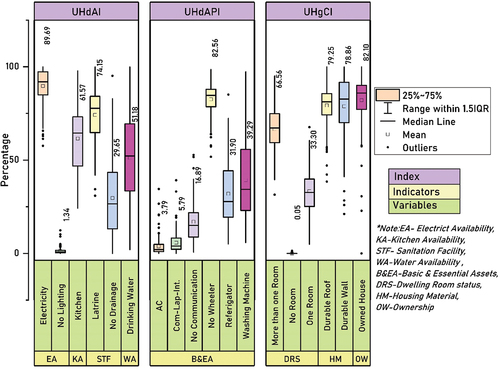
Table 2. Summary statistics of the selected variables.

Variables	Mean	SD	CV	Maximum	Minimum	95% CI Mean
Wall	78.86	16.0	20.23	100	21.1	(76.3,81.4)
Roof	79.25	11.5	14.48	100	38.5	(77.4,81.1)
Ownership	82.10	13.7	16.64	100	0.00	(79.9, 84.3)
No Room	0.05	0.14	299.36	1.42	0.00	(0.0249, 0.0717)
One Room	33.3	11.0	33.08	67.7	4.87	(31.5, 35.1)
More Room	66.6	11.0	16.55	95.1	31.4	(64.8, 68.3)
Drinking Water	51.2	22.0	43.7	100	1.98	(47.6, 54.8)
Kitchen	61.6	16.6	26.89	97.8	24.2	(58.9, 64.3)
No Light	1.34	1.74	130.22	13.3	0.00	(1.05, 1.62)
Electricity	89.69	9.52	10.61	100	57.6	(88.1, 91.2)
No Waste Outlet	29.7	19.9	66.97	95.2	0.00	(26.4, 32.9)
Latrine	74.1	14.4	19.38	100	30.9	(71.8, 76.5)
Refrigerator	31.9	15.7	49.15	85.1	5.04	(29.4, 34.4)
No Communication	16.9	10.8	64.01	52.8	0.72	(15.1, 18.6)
Computer	5.78	5.38	93.91	0.00	37.7	(4.91, 6.66)
No Wheelers	82.6	8.44	10.22	98.6	51.8	(81.2, 83.9)
Air Conditioner	3.79	4.88	128.94	34.5	0.00	(3.00, 4.58)
Washing Machine	39.29	20.5	52.17	97.3	5.77	(36.0, 42.6)

The Coefficient of Variation (CV) of 18 indicators shows that most disparities among the urban centres existed in terms of no room (CV = 299.36), followed by no light (CV = 130.22), Air Conditioner (CV = 128.94) (Table 2). On the other hand, the least inter-urban household living condition disparities are found on no-wheelers (CV = 10.22), followed by electricity (CV = 10.61) and durable roofs (CV = 14.48). It shows that West Bengal’s urban centres are variably developed in different indicators of household living conditions but with certain limitations. Additionally, the difference between the regions with the best and worst performers in terms of these indicators is widened.

3.2. Clustering pattern and spatial variations

3.2.1. Clustering pattern and spatiality of urban housing condition

Housing conditions include the physical structure that provides accommodation, the immediate neighbourhood, the relevant community infrastructure and assistance, and the surroundings of the building, which includes all services and facilities preferred for the family’s and individual’s social, physical, and mental well-being (Firdaus and Ahmad 2013). The impediments to prosperity include inequalities, asymmetrical growth, lack of infrastructural development, limited government support, and a lack of utilities and services that affects the living condition and well-being status of the urban inhabitants (Bhagat 2011; Das and Mistri 2013). Figure 4a-f shows the clustering pattern of the selected indicators of urban housing condition, which includes durable roof, durable wall, owned house, house with no room, one room, and multiple rooms (Table 3). Notably, the greater the Z-score value, the more intensive the clustering pattern of high values, i.e. hot spot, and the lower the Z-score indicates the more concentration of low values, i.e. cold spot. The variation in red colour (from dark to light) indicates statistically significant hotspot urban centres with 99%, 95%, and 90% confidence. Similarly, the deviation in blue colour indicates variation in coldspots with different confidence rates. However, the grey colour indicates the statistically insignificant urban centres.

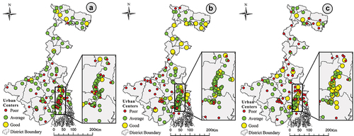
Figure 4. Spatial pattern of selected variables used for the present study. (a-f) Urban housing condition variables which includes predominant material of roof (RF), predominant wall materials (WA), ownership status (OS), No room (NR), one room (OR), and more than one room (MOR); (g-l) Urban household amenities variables which includes drinking water (W), kitchen availability (KT), electricity availability (EL), no electricity (NE), no waste water-outlet (NWO) connections and water-seal latrine facility (LT); (m-r) Urban household asset possession variables which includes availability of air conditioner, refrigerator (RF), no communications (NCM), no motorize wheelers (NW), washing machine (WM) and computer/laptop availability (CL).

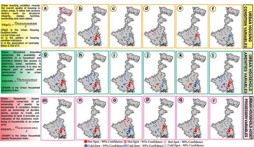
Table 3. Variable-based Moran’s I index, z-score, and pattern of spatial association.

Index	Variable	Moran’s I	z-score	Pattern
Housing Quality Index	Wall	0.29*	21.88	Clustered
	Roof	0.03*	2.96	Clustered
	Ownership	0.02*	1.98	Clustered
	No Room	0.00	0.266	Random
	One Room	0.03*	3.30	Clustered
	More Room	0.03*	3.23	Clustered
Household Amenities Index	Drinking Water	0.15*	11.85	Clustered
	Kitchen	0.22*	17.27	Clustered
	No Light	0.05*	4.72	Clustered
	Electricity	0.33*	25.17	Clustered
	No Waste Outlet	0.17*	12.96	Clustered
	Latrine	0.25*	19.00	Clustered
Household Assets Possession Index	Refrigerator	0.25*	18.78	Clustered
	No Communication	0.31*	23.64	Clustered
	Computer	0.16*	12.90	Clustered
	No Wheelers	0.07*	5.87	Clustered
	Air Conditioner	0.15*	11.75	Clustered
	Washing Machine	0.14*	10.83	Clustered

Note *: the corresponding significance level (p-value) is < 0.001.

For example, Figure 4a reveals the durable roof conditions in 146 urban areas of Eastern India. According to the study findings, the municipalities in the northern part, like Kurseong, Mekhliganj, Dinhata, Siliguri, Coochbehar, Kalimpong, Tufanganj, and so on have high hotspots cluster with high z-score values, which varies between 2.86 and 3.93. Interestingly, these 15 municipalities in the northern region have a maximum percentage of households (94.45% to 99.67%) with a durable roof. In contrast, the urban centres in the south-central part with a maximum number of coldspot municipalities include Beldanga, Rampurhat, Kandi, Berahampore, Murshidabad, and so on, with a z-score value between −1.77 and −2.88. It indicates that the south-central part of the study area has a low concentration of the durable house.

Similarly, the clustering pattern of a durable wall (Figure 4b) depicts that the municipalities like South Dumdum, Kalua, Sajnaberia, Diamond Harbour, Howrah, Kolkata, Budge Budge, Rishra, Bally, and so on have high hotspot values (z-score between 1.99 and 6.46) which were concentrated on the southeastern part of the study area. It indicates that these urban areas have the maximum number of households with the predominant material of the roof, which is durable. In contrast, the coldspots areas are concentrated mainly in the southwestern parts, with z-score values varying from −1.44 to −5.36. However, Figure 3c shows that most urban areas have an insignificant cluster of owned houses, only urban centres in the southeastern part (with a z-score value of −1.66 to −3.64) showing clusters of coldspots.

In the case of Figure 4d (with no rooms), again, the majority of the urban centres show insignificant clusters. Interestingly, the urban centres in the southwestern part, like Jamuria, Bankura, Kulti, Sonamukhi, Dubrajpur, Suri, Raniganj, Raghunathpur, and so on, have high clusters of hotspots. These urban centres are concentrated in the Paschim Bardhaman, Puruliya, Bankura, and Birbhum districts of the study area. According to the previous studies of Das (2018), Sarkar (2019), and Chandra (2021), these districts in the western part are underdeveloped in terms of poor infrastructure development, socio-economic deprivation, and high incidence of poverty. Interestingly, Figures 4e,f (household with one room and more than one room) have an inverse relationship. In the case of Figure 4e the hotspots with high clustering patterns of households with one room found in the southeastern part (with a z-score value of 1.59 to 3.07) and coldspots clustered in the north-western part of Kurseong, Kalimpong, Darjeeling, and Mirik Municipality (z-score value of −2.33 to −3.98). The situation reversed in the case of Figure 4f as the hotspots with high clustering patterns of households with more than one room were found in the north-western part, and coldspots clustered in the southeastern part. It indicates that if the urban centres have less number of single rooms, then it means that urban centres have households with the availability of multiple dwelling rooms.

Based on the above-mentioned six housing condition indicators, an aggregated normalized UHgCI is constructed to reflect the overall dwelling condition in an urban area. Figure 4a shows the proportionate symbol of spatial variations in UHgCI with three classes poor, average and good. According to the calculated index values, 35 urban centres (23.97%) have poor urban housing conditions. The bottommost urban centres with poor UHgCI are mainly concentrated in the southern part, namely, Beldanga, Maheshtala, Arambag, Kamarhati, Kharagpur, Kalyani, Gobardanga, Chandrakona, Birnagar, and Gayespur (Figure 5a). On the other hand, majority of 96 urban centres (65.75%) with average index values are unevenly distributed within the study area (SL Table 1). In contrast, Figure 4a reveals that only 10.27% (15) urban centres in Eastern India have overall good urban housing conditions. The top 10 urban centres with decent UHgCI were Jamuria, Sajnaberia, Tufanganj, Santipur, Old Malda, Ramchandrapur, Siliguri, Uttarpara Kotrung, Pujali, and Jalpaiguri.

Figure 5. Thematic variations of computed sub-indexes (a) Urban Housing Condition index (UHgCI); (b) urban household amenities (UHdAMI); and (c) urban household assets possession (UHdAPI).

3.2.2. Clustering pattern and Spatiality of Urban household amenities

In order to raise the living standard and promote people’s well-being, accessibility to essential urban amenities such as clean water, drainage facility, sanitation, and electricity are crucial factors (Das, Das, and Barman 2021; Parry, Ganaie, and Bhat 2018). However, according to previous studies, West Bengal has a significant gap in access to essential utilities compared to many other areas in the global South (Mondal 2020; Mondal and Das 2022), but none have tried to identify the clustering pattern and spatial variations at the municipality, corporation, cantonment board or notified town area level of urban centres.

Interestingly, Figure 4g,h,i & l and Table 3 reveal a similar pattern of hotspots clustering in the southeastern part of the study area around the Kolkata megacity and coldspots clustered along the southern and southwestern part of the Paschim Bardhaman, Paschim Medinipur, Puruliya, Bankura, and Birbhum districts. It reveals that access to basic amenities is more concentrated around the megacity region because these areas tend to have larger populations and higher densities, which can support a broader range of facilities and services (Hosseini et al. 2021). Also, the southeastern part tends to have more developed infrastructure and a more robust economy, which can support the development and maintenance of urban utilities. Additionally, these urban areas along Howrah, Hugli, Kolkata, and North 24 Parganas are often more accessible and connected, making it easier for residents to access amenities; as a result, urban residents may have more options and opportunities for accessing amenities than rural residents.

According to Figure 4g., the spatial clustering pattern of drinking water availability within the premises with high z-score values of 2.07 to 6.34 was considered as hotspot zones, which was found in urban centres of Nabadiganta industrial town, Khadra, North Barrackpore, Santipur, Barrackpore, Ranaghat, Madhyamgram, Chandannagar, Kalyani, Barasat and so on. While the coldspots (z-score value between −1.75 and −4.37) urban centres in the southwestern part include Jhalda, Kulti, Jamuria, Puruliuya, Dubrajpur, Raghunatpur, Bankura, and southern part includes Chandrakona, Panskura, Kshirpai, Haldia, Medinipur, Ghatal, Arambag and so on. Similarly, the cluster of Figure 4h shows the availability of the kitchen with maximum hotspot values of 2.58 to 5.37 and minimum coldspots value of −1.68 to −3.59. Figure 4i shows a clustering pattern of electric availability with a high z-score value (hotspots) of 1.33 to 6.92 and a low z-score value (coldspots) of −0.75 to −3.62. Moreover, Figure 4l shows a similar pattern of water-sealed latrine facilities with hotspot clusters between 1.06 and 5.89 and coldspots cluster between −0.98 and −4.35.

Interestingly, Figure 4j depicts the spatial cluster of households with no source of electricity, which reveals that high hotspots (z-score value 1.60 to 3.81) were concentrated in urban centres of the central part (viz. Dhulian, Jangipur, Old Malda, Rampurhat, Englishbazar, and Naihati) and southern parts (viz. Jhargram, Medinipur, Egra, Kharagpur, Kulti, Kharar, Chandrakona, Ghatal, and Ramjibanpur). In contrast, the urban centres around the Kolkata megacity area have been identified as coldspots urban centres with a low z-score value of −1.01 to −2.76.

The analysis of category-wise amenities level of urban households and the nature of the spatial distribution is illustrated in Figure 5b. A composite synthetic index for urban amenities is constructed for spatial analysis, i.e. UHdAMI. The results indicate Dum Dum has good household amenities availability with an estimated UHgCI value of 1, whereas, Kshirpai municipality of Paschim Medinipur district is the least availability of household amenities with an estimated normalized UHgAI value of 0. The urban centres with a good position of UHdAMI are Dum Dum, Krishnanagar (0.737), Gopalnagar (0.674), Sajnaberia (0.671), Raiganj (0.640), and so on. According to the findings, about 33 urban centres (22.60%) were positioned under the good amenities holding category, where the majority of the urban centres are distributed over the northern part of West Bengal (Haldibari, Tufanganj, Islampur, Mathabhanga, Dinhata, English Bazar, Raiganj, KochBihar, Balurghat, Gangarampur). In contrast, the state’s southern and southeastern parts consist of urban centres like Santipur, Chakdaha, Taherpur, Halisahar, Tarakeswar, and so on. Furthermore, around 54.79% of urban centres in the state emerged as a moderate level of urban household amenities. These moderate UHdAMI is mainly distributed in the southern part of the study area, or more precisely, a high concentration is located around the capital city of Kolkata. Also, a few moderate levels of UHdAMI are sparsely located in the extreme southwest, central, and northern parts of West Bengal. On the other hand, the low level of UHdAMI covers 33 urban centres, mainly distributed over the study area’s southern, central, and western parts. The findings indicate that most of the urban households live in the western part of the states, namely, Ramjibanpur, Dubrajpur, Nalhati, Guskara, Jhalda, Raghunathpur, Sonamukhi, Bankura, Jamuria, Chandrakona, Puruliya, Kulti facing the issue of poor amenities level, means the household are not well equipped to basic utilities that enhanced their living standard to boost the human resource level and meet the criteria of sustainable development.

3.2.3. Clustering pattern and spatiality of urban household assets possession

Household asset possession refers to household property ownership, including a wide range of material things and wealth, such as property, vehicles, household goods, and financial investments (Traynor and Raykov 2013). The level of asset possession can vary significantly among households and can be an essential factor in determining a household’s financial stability and well-being. In general, households with a higher level of asset possession are likely to have more financial security and be better able to withstand financial challenges (Mondal 2020; Punia and Kaushik 2018). The possession of assets can also provide households with opportunities for economic growth and development (Harttgen, Klasen, and Vollmer 2013).

According to Figure 5m-r the clustering pattern of hotspots is concentrated in the southern, eastern part along the Kolkata megacity region. For example, Figure 3m represents the spatial clustering of households with air condition availability with the maximum z-score value varying between 2.64 and 5.21 and the lowest value between −1.01 and −2.31. Similarly, Figure 5n (household with refrigerator availability), Figure 4q (households having washing machines) and Figure 5r (household with laptop or computer availability) showing spatial cluster with high z-score value (hotspot) of 1.42 to 6.36, 1.03 to 4.96, and 1.59 to 4.91, respectively. In contrast, the coldspots for these three figures were clustered in the southern part with low z-score values varying between −1.42 and −3.03, −1.17 and −2.73, and −1.70 and −2.24, respectively. Interestingly, Figure 4o represents the variation of clustering patterns in households with no modern communication facilities, including landline and mobile. It reveals that the hotspots’ urban centres were located in the northern part (including Coochbehar, Raiganj, Mathabhanga, Dhupguri, Jalpaiguri, Kaliyaganj, Dalkhola, and Gangarampur), the south-central part (comprises Dhulian, Jangipur, Kandi, Jiaganj-Azimganj, Rampurhat, Murshidabad, Sainthia, Nalhati and so on), and the southwestern part (includes Guskara, Jamuria, Kulti, Sonamukhi, Bolpur, Puruliya and so on). All these municipalities were somewhat underdeveloped in terms of modern communication compared to the urban centres in the southeastern part. It is mainly due to the urban areas in the southeastern part around the Kolkata megacity (coldspots) having better access to modern communication technologies and supporting higher services due to a maximum population density and level of economic development, and solid infrastructure base.

Furthermore, based on these six asset possession indicators, a composite normalized UHdAPI is constructed, which reflects the composite level of assets for the households (Figure 5c). From the computed results, Paschim Putiary, Dum Dum, Khardah, South Dum Dum, and Uttarpara Kotrung were identified as the top five urban centres in terms of UHdAPI value ranges from 0.600 to 1, respectively. Out of the 146 urban centres, 33.56% (49) of urban centres fall under the good category of urban household assets possession level, and these areas are mainly located in the southern part of the state, near Kolkata and its adjacent area. Also, some urban areas in the upper central and northern parts of the state fall under good levels of UHdAPI. Similarly, 34.25% of the urban centres are sparsely distributed in the different parts of the state and are identified as moderate levels of asset possession by urban households. The top-bottom urban centres with a low level of UHgCI are mainly concentrated in the southern part (Coopers Camp, Gopalnagar, and Dhulian) and some parts of northern Bengal (Dalkhola, and Gangarampur). Additionally, 32.19% (47) of urban centres have poor household possession assets distributed over the southern part, central part, and unevenly located in the northern part of West Bengal.

3.3. Hotspot analysis and spatial autocorrelation using Moran’s I

3.3.1. Spatial characteristics of UHgCI

The hotspot analysis of Figure 6a reveals that only a few urban centres, namely, Siliguri, Kurseong, Mirik, Kalimpong, Darjeeling, and Mal in the north and Raniganj, Jamuria, Kulti, and Raghanathpur in the southwestern part has clustering pattern with a high z-score value between 1.77 and 1.80. Interestingly, no coldspot urban centres were identified, and most of the municipalities and cantonments were statistically insignificant.

Figure 6. Hotspots & coldspots showing spatial clustering pattern, autocorrelation and zonal distribution of computed sub-indexes. (a-c) UHgCI, (d-f) UHdAMI, (g-i) UHdAPI.

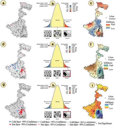
Moreover, Figure 6b shows the autocorrelation pattern with Moran’s I value of 0.004 and a z-score value of 0.85 with a significance level of 0.39. Therefore, the study area’s final urban housing condition index reveals a random spatial pattern. On the other hand, Figure 6c reveals the district-level spatial distribution of the UHgCI, which reveals urban centres in northern districts (like Darjeeling, Jalpaiguri, Kalimpong Coochbehar, and Alipurduar), southeastern districts (Kolkata, Howrah, South 24 Parganas, and upper part of Purba Medinipur) and western district like (Lower part of Birbhum, Paschim Bardhaman, and upper part of Bankura) has high z-score value, which signifies an excellent urban housing condition.

3.3.2. Spatial characteristics of UHdAMI

Figure 6d represents the spatial pattern of UHdAMI across the study area, which reveals that urban centres like Alipurduar, Tufanganj, Mathabhanga, Dinhata, and Gangarampur in the northern part has hotspots with high z-score value. On the other hand, the southeastern part comprises Chakda, Panihati, Barrackpore, Serampore, Chandannagar, Naihati, Rishra, Barasat, Kalyani, Madhyamgram and so on, with high hotspot values which vary from 2.82 to 3.51. In contrast, the southwestern and southern part comprises urban centres like Puruliya, Bolpur, Suri, Jhalda, Kulti, Saithia, Guskara, and so on have been identified as coldspots with a low z-score value between −2.25 and −4.07.

According to Figure 6e, Moran’s I value of 0.71, and z-score value of 5.71 with a significance of 0.00 level reveals that the urban amenities index of the study area shows a spatial clustering pattern. Besides, the district-level analysis shows Alipurduar, Coochbehar, a few parts of Jalpaiguri, North and South Dinajpur in the northern part, and districts around the Kolkata capital region in the southeastern part showing a high level of UHdAMI (Figure 6f). Interestingly, parts of Murshidabad, Birbhum, Puruliya, Bankura, Paschim Bardhaman, and hilly parts of Darjeeling and Kalimpong districts show a tendency of low UHdAMI. It is because the megacity region of Kolkata usually has more amenities compared to other parts; as a result, urban centres in the southeastern part tend to have a higher utility availability. On the other hand, smaller urban centres may not have as many amenities, resulting in lower values.

3.3.3. Spatial characteristics of UHdAPI

Figure 6g that only the southeastern part of the study area has high hotspot urban centres with values ranging from 1.80 to 6.65. It is because asset possession, which measures the ownership of assets such as vehicles, electronics, and furniture, is typically highest in large urban centres like Kolkata, Barasat, Diamond Harbour, Howrah, Haldia, Bally, Barrackpore, Budge budge, Chakda, Chandannagar, Dum dum, Joka, Kanchrapara, Naihati, Rishra, Taki, and so on compared to other smaller urban centres. The higher incomes and higher levels of consumption associated with such larger urban centres, coupled with the availability of a wide range of goods and services and developed infrastructure consequence in a wide range of urban assets. The urban centres with coldspots (−1.55 and −2.41) are mainly found in the central and southern parts, namely, Berhampore, Murshidabad, Raiganj, Birnagar, Bishnupur, Dhulian, Ghatal, Katwa, Medinipur, and so on.

According to Figure 6h, the UHdAPI of the study area shows a clustered pattern with Moran’s I value of 0.29 and a z-score value of 21.71 with a 0.00 significance level. Besides, the district-level spatial variation of UHdAPI reveals that except Kolkata, Howrah, Hugli, North and South 24 Parganas, all other districts have moderate to low UHdAPI (Figure 6i).

3.4. Spatial pattern of the final Urban household condition of living index (UHdCLI)

Living conditions are the aspects or contexts that influence the way people survive, especially when it comes to their well-being (El-Bialy and Mulay 2015; Zhang, Zhang, and Hudson 2018). The words ‘living conditions’ and ‘quality of life’ are often used together (Boelhouwer 2002). Here, it signifies the degree to which an urban household is productive, satisfied, and capable of participating in a potential developmental process. Calculating the household living status typically involves collecting data on various indicators relevant to living conditions. These indicators may include income and wealth, education, housing, health, and access to services such as electricity, water, and sanitation (Ghosh and Roy 2022; Mberu 2007). In the present study, UHdCLI is computed based on the three discussed sub-index, i.e. UHgCI, UHdAMI, and UHdAPI, which reflects the overall living conditions experienced by households. The indicators of UHdCLI categorically include housing environment, amenities level, and assets held by the urban households. These indicators critically assess the intensity of urban household well-being status and produce a comparable result to visualize the spatial heterogeneity of quality distribution of household living condition level (Figure 7).

Figure 7. Spatial variation of Composite Urban household condition of living index (UHdCLI). (a) Thematic variation of UHdCLI based on index value, (b & c) spatial pattern and autocorrelation of UHdCLI (d) district wise spatial zonation of UHdCLI.

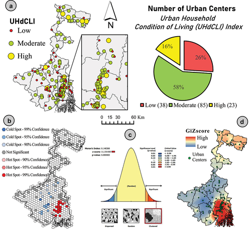
The result of UHdCLI ranges between 0.141 and 0.712, which is further categorized under three distinctive living condition levels (Figure 7a), namely, low (0.141–0.331), moderate (0.332–0.521), and high (0.522–0.712). The findings show that the highest UHdCLI value is recorded for Uttarpara Kotrung (Hugli district) with an estimated UHDCLI value of 0.712, followed by Sajnaberia (0.708), PurbaBarisha (0.577), Ramchandrapur (0.577), Paschim Putiary (0.578), Khardah (0.580), Krishnanagar (0.590) Tufanganj, (0.591), North Dum Dum (0.611), DumDum (0.692), and so on. According to the calculated index values, 25 urban centers (23.97%) have high urban household living conditions. These urban areas are mainly concentrated in the southern part, adjacent to the state’s capital. It can be attributed to the fact that these urban centres majorly work as a critical node for most of the socio-economic activities and provide better access to the services provided by urban administration. There is an evident influence of the locational advantage of these large urban centres, which can motivate the living condition and access to the essential amenities for the majority of urban households (Table 4). Only four urban centres (Siliguri, Jalpaiguri, Tufanganj, and Koch Bihar) are from the northern part of West Bengal has good UHdCLI.

Table 4. Spatial zonation based on GiZ by inverse distance weighted (IDW) interpolation based on urban household condition of living index (UHdCLI).

Spatial Zonation based on GiZ by inverse distance weighted (IDW) interpolation
Zone of High-High Value	Zone of Low-Low Value
(a) Kolkata Municipal Corporation and surrounding urban areas. (b) Majority part of North 24 Paragana, Howrah, Southern Part of Nadia. (c) All most all part of South 24 Paragana, and very small north eastern part of Paschim Medinipur District. (d) Whole Darjeeling, Jalpaiguri, Alipurduar, Coochbehar, and upper most part of Uttar Dinajpur. (51.29%)	(a) Almost all part of Murshidabad, Birbhum, Bankura, Puruliya and Bardhaman district (b) Sparsely identified in Purba and Paschim Medinipur District. (c) Upper part of Nadia, part of Maldah, and Dakshin Dinajpur. (47.56%)

One key determinant contributing to this concentration is the function of these urban centres as vital nexus points for socio-economic endeavours. Due to their proximity to the state capital, these urban hubs tend to attract economic investments, employment prospects, and infrastructural advancements. They serve as thriving epicentres for commerce, trade, and industries, thereby fostering augmented incomes and an enhanced standard of living among residents (Haque, Mehta, and Kumar 2019; Mondal and Banerjee 2021; Sengupta and Tipple 2007). Additionally, the presence of well-established urban administration and governance structures in these locales facilitates improved accessibility to services and amenities (Mondal 2021; Roy et al. 2023). Urban centres situated near the state capital frequently benefit from heightened levels of urban planning efficiency alongside superior provision of infrastructure and public services such as healthcare facilities, educational institutions transportation networks, and recreational spaces (Cattaneo et al. 2022; Jain and Korzhenevych 2020). All these factors collectively contribute towards a more favourable quality of living conditions within urban households residing in the study area. Furthermore, the advantageous geographical positioning enjoyed by these larger urban centres plays a significant role in motivating superior household living conditions (Glaeser et al. 2018). Their close proximity to major transportation corridors commercial districts, and public amenities endows residents with convenient access to opportunities markets, social services, and recreational facilities. This heightened accessibility significantly enhances overall well-being and living standards. The concentration of high-quality urban household living conditions observed within these regions finds empirical support from previous studies on urban dynamics. Research has consistently demonstrated that those urban centres which operate as economic powerhouses administrative nerve-centres exhibit elevated levels of economic prosperity, optimal infrastructural provision along with enhanced accessibilities towards public services (Haque, Mehta, and Kumar 2019; Mondal and Banerjee 2021). Hence, the clustering phenomenon pertaining to urban regions exhibiting superior living conditions within the southern part of the study area, particularly those adjoining the state capital, is attributable to their pivotal role as vital nodes for socio-economic activities coupled with their enhanced accessibilities towards services provided by urban administrative structures.

On the other hand, the majority of 81 urban centres (55.48%) with average UHdCLI values are unevenly distributed within the study area. However, a significant concentration of the moderate value of composite living conditions is recorded in the southern part of the study area, adjacent to the high UHdCLI urban centres. Moreover, the least UHdCLI is noted for Beldanga municipality (0.141) of Murshidabad district, followed by Ramjibanpur (0.162), Chandrakona (0.167), CoopersCamp (0.176), Jhalda (0.186), Dhulian (0.191), Birnagar (0.193). Figure 4C shows that urban centres with the lowest household living condition located in the southern part, the southwestern part, the extreme western part, the central part, and some parts of northern West Bengal. Interestingly, only three urban centres in the extreme north and hilly part of the state, Darjeeling, Alipurduar, and Dalkhola, faced various issues regarding the urban household living condition. Another concerning fact is that major urban centres and potential economic hubs of West Bengal, i.e. Asansol, also experienced a poorer level of the overall living condition experienced by the urban inhabitants.

The spatial distribution of urban centres exhibiting poor household living conditions in West Bengal showcases discernible patterns, which can be ascribed to a multitude of factors encompassing geography, environment and access to indispensable services within these locales. In the farthest reaches of northern part, characterized by undulating topography, rugged landscapes and deficient infrastructural amenities, urban hubs encounter manifold challenges in ameliorating their living conditions. The formidable terrain presents hindrances to infrastructural progressions, provision of services and accessibility; thereby amplifying the difficulties faced by urban households (Mondal 2020; Roy et al. 2023). Furthermore, the southernmost and westernmost regions including coastal areas are beset with harsh geo-environmental circumstances. These territories are prone to coastal perils such as cyclones, storm surges and inundation events that heighten vulnerability among households residing there. The deleterious ramifications inflicted upon infrastructure, livelihoods, and overall living standards stand evident (Bagli and Tewari 2019; Ghosh and Mistri 2021; Majumder et al. 2023). Moreover, the restricted availability of essential services exacerbates the substandard living conditions experienced by urban households in these regions. In addition to geographical and environmental determinants, some parts from north-western extremities suffer from limited accessibility towards imperative services. These areas may grapple with insufficient healthcare provisions, economic opportunities, potable water sources, and sanitation facilities (Majumder et al. 2022; Mondal and Das 2022). The hurdles associated with provisioning adequate infrastructure alongside public services stem from factors like remote locations, diminished population density or constrained economic resources (Roy et al. 2023).The cumulative impact precipitated by these elements contributes towards lower UHdCLI values observed across these realms. The difficult terrain, challenging environmental circumstances along with curtailed accessibilities towards vital services collectively engender impoverished living conditions while impeding the well-being of urban households.

Furthermore, Figure 7b depicts that the urban hotspot centres with high z-score value (1.66 to 4.89) were clustered in the southeastern part, and the coldspot urban centres with low z-score value (−1.70 to −2.83) was distributed in the southern part. Therefore, the results revealed that the study area’s overall UHdCLI (Figure 7c) was not randomly distributed, but it was explicitly clustered due to some locational advantages in the southeastern part (Morans’I = 0.14, z-score value = 11.19 with 0.00 significance level). However, the district-wise spatial pattern of UHdCLI reveals that the urban centres in the southeastern districts like Kolkata, Howrah, Hugli, North and South 24 Parganas have a high level of urban household living conditions (Figure 7d). Besides, the urban centres in the northern part comprise high to moderate levels of UHdCLI distributed in the districts of Darjeeling, Kalimpong, Jalpaiguri, Alipurduar, and Coochbehar. On the contrary, the central and southwestern part of the study area comprises low UHdCLI.

3.5. Correlation among the constructed indexes and model consistency

Figure 8 illustrates the Pearson correlation with adjusted R² among the Constructed Indexes (UHgCI, UHdAMI, UHdAPI, and UHdCLI) in the study, where the degree of association and amount of variance explained by these components are highlighted. The correlation coefficients represented strong statistical association among the sub-indexes with the final composite index and explained enough variance. Interestingly, Figure 8 reveals that UHgCI is less positively correlated with UHdAMI and UHdAPI and explained significantly less extent of variance. The illustration of the correlation matrix in this figure shows that in UHdCLI and UHgCI; UHdCLI and UHdAMI; UHdCLI and UHdAPI, the correlation coefficient were high. Among them, UHdAPI explains the largest amount of variance (approximately 61.19%) of computed UHdCLI. On the other hand, other indexes are also partially correlated with each other.

Figure 8. Scatter matrix plot showing the Pearson’s correlation with adjusted R² for the constructed UHgCI, UHdAMI, UHdAPI and UHdCLI. The ellipse showing the distribution of Urban centres with 95% confidence.

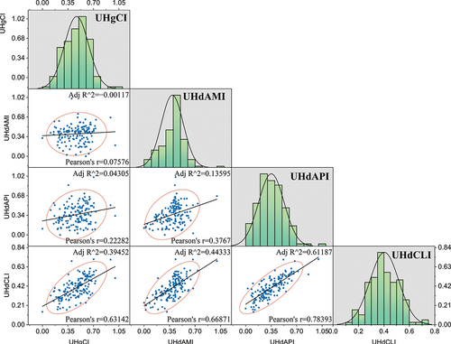
Furthermore, the constructed UHCLI model’s consistency is assessed using the r-squared value of regression analysis (Musse, Barona, and Rodriguez 2018; Roy et al. 2022). For that purpose, six variables are employed from three sub-indices based on the highest and lowest coefficient of variation (CV) value. roof, no light, and air conditioner is selected as a predictor variable of UHdCLI for the highest CV on the respective domain, while no room, electricity, washing machine is selected as the predicted variable for the lowest CV on the respective domain. The regression outcome results (Table) indicate that the constructed model is acceptable since it accounts for almost 82% of the variance of the developed UHCLI index, with a corresponding R² value of 0.815 (Table 5). Hair et al. (2011) suggest that R² value greater than 0.75 significantly predicts the input model and provides consistent results. Also, all six outcome variables significantly predict the model at a 0.05 significance level.

Table 5. Summary of regression analysis for model consistency.

Model	Predictors	Coefficients	R^2	t	Significance
UHdCLI	Roof	.302	0.815	5.330	.000
	No Room	−.169		−2.208	.004
	Electricity	.609		9.308	.000
	No Light	−.293		−4.504	.000
	Air Conditioner	.304		5.358	.000
	Washing Machine	.123		2.139	.034

4. Conclusion

The present findings provide a realistic view of the spatial inter-urban variations that exist at the level of particular households concerning several aspects of their standard of life. The proposed framework for assessing urban household living conditions utilized several interconnected socioeconomic indicators to derive the ultimate spatial output of the living status of the selected urban centres in West Bengal. Here, three distinct sub-dimensions (i.e. UHgCI, UHdAI, and UHdAPI) synchronized by the proposed method were quite distinctive, justified and easy to apply in other regions. This study’s methodological approach was considered a beneficial tool for analyzing the geographical heterogeneity of development requirements in various urban locations worldwide. However, the choice of variables is the most critical aspect for this type of application, where the output depends significantly on that specific region’s social, economic, urban locality, and geographic characteristics. The study’s outcome reveals that the towns close to Kolkata led to better financial facilities, access to basic amenities, and more efficient urban service delivery systems. The rest of the smaller towns endures enormous disadvantages as they have been trapped at a persistently backward level of infrastructural development. Despite being distant from Kolkata, the urban development criteria substantially influence the urban living inequality scenario of the comparatively less urbanized regions in the northern and western parts of the state.

The applied research procedure allowed us to identify the potential areas with minimum household living conditions in different-sized urban areas spread across West Bengal. The segmentation of the best-performing municipalities to the worst-performing ones facilitated by identifying spatial inequality among urban centres enabled even more targeted interventions to be developed. In this study, the selected variables replicate the inherent scenario of city dwellers’ living conditions and potential bottlenecks. The heterogeneity context is explicitly highlighted, and well-being status is measured utilizing the synthetic index creation approach. The outcome significantly identifies the spatial variability in the living condition of urban inhabitants in the study area, which helps to formulate dedicated developmental programmes and improvements in human, social, and physical capital of the urban households in target-based manner. The findings suggest an uneven household well-being scenario across the study area’s different geographical locations. Furthermore, the municipalities adjacent to the capital city and mainly located in the central part of the state experience better living conditions than their counterparts. The neighbourhood influence was substantially connected with the well-being of households; therefore, the researchers and policymakers need to focus on that aspect when developing and implementing urban livelihood development strategies.

Despite its substantial contribution to understanding the spatial variations in household conditions and heterogeneity among urban dwellers, the study has a few limitations. Due to data constraints, a few additional factors related to urban housing living conditions could not be employed. Therefore, based on the current approach, a larger comparative study is possible among the different urban centres worldwide that would help identify the inter-regional (neighbourhood) influence on urban household living conditions. Besides, for future studies, knowledge and perceptions of the urban residents could provide a better understanding of the spatial variations in housing living status. Despite these few limitations, this study’s methodological approach and results can provide the researcher with a clear concept of spatial heterogeneity, and it can be applied on a large scale. The outcome of the composite index with the integration of GIS technology is a powerful tool for analyzing and visualizing spatial patterns. The present study also proves that GIS can effectively map and analyze the households living conditions in urban areas. The current approach can benefit planners, policymakers, and researchers to understand better the households’ conditions in different parts of the world and to identify areas that may require intervention or support.

Credit authorship

S.R. S.M. and A.B.- Supervision, Writing Original Draft, Conceptualization, Formal analysis, Investigation, Methodology, Software, Visualization, Review & Editing; I.R.C -Review & Editing. All authors have read and agreed to the published version of the manuscript.

Acknowledgements

The author wishes to thank the Department of Geography and Applied Geography, University of North Bengal (India), for providing the necessary facilities to carry out this study. This research was completed during the tenure of UGC-JRF. The authors would like to acknowledge all the Governmental reports and data with which it is possible to find such novel results. Besides, the authors would like to sincerely thank the editor-in-chief Dr A-Xing Zhu for the insightful remarks. Also, the insightful comments from the two anonymous reviewers greatly assisted in improving the manuscript. Lastly, the authors would like to thank Nanjing Normal University for supporting the APC.

Disclosure statement

No potential conflict of interest was reported by the author(s).

Data availability statement

The governmental data used in this study is freely available from SECC, India.

References

- Abante, A. M. R. 2020. “Risk Hotspot Conceptual Space Characterized by Hexagonal Data Binning Technique: An Application in Albay, Philippines.” International Journal of Computing Sciences Research 5 (1): 550–567.
- Abante, A. M. R. 2021. “Geophilosophical Realness of Risk: A Case Study in National Housing Authority Resettlement Sites in Albay, Philippines.” SN Applied Sciences 3 (4): 1–22. https://doi.org/10.1007/s42452-021-04442-6.
- Agarwal, S., T. P. Singh, D. Bajaj, and V. Pant. 2021. “Affordable Housing in Urban India: A Review of Critical Success Factors (CSFs) Addressing Housing Adequacy with Affordability for the Urban Poor.” Housing, Care and Support 25 (1): 61–79. https://doi.org/10.1108/HCS-08-2021-0022.
- Ahluwalia, I. J. 2019. “Urban Governance in India.” Journal of Urban Affairs 41 (1): 83–102. https://doi.org/10.1080/07352166.2016.1271614.
- Ahmed, N., and J. H. Khan. 2018. “Spatial Distribution of Availability of Household Amenities in Scheduled Tribe Population in India.” International Journal of Research in Humanities, Arts and Literature (IMPACT: IJRHAL) 6 (8): 239–250.
- Ansary, R., and B. Das. 2018. “Regional Patterns of Deprivation in India: An Assessment Based on Household Characteristics, Basic Amenities and Asset Possession.” Social Change 48 (3): 367–383. https://doi.org/10.1177/0049085718781663.
- Anselin, L., S. Sridharan, and S. Gholston. 2007. “Using Exploratory Spatial Data Analysis to Leverage Social Indicator Databases: The Discovery of Interesting Patterns.” Social Indicators Research 82 (2): 287–309. https://doi.org/10.1007/s11205-006-9034-x.
- Bagli, S., and G. Tewari. 2019. “Multidimensional poverty: an exploratory study in Purulia district, West Bengal.” Economic Affairs 64 (3): 517–527. https://doi.org/10.30954/0424-2513.3.2019.7.
- Behera, D. K. 2016. “Measuring Socio-Economic Progress in India: Issues and Challenges.” Revista Galega de Economia 25 (2): 117–132. https://doi.org/10.15304/rge.25.2.3742.
- Bhagat, R. B. 2011. “Urbanization and Access to Basic Amenities in India.” Urban India 31 (1): 1–14.
- Bhattacharjee, K., and B. Behera. 2018. “Determinants of Household Vulnerability and Adaptation to Floods: Empirical Evidence from the Indian State of West Bengal.” International Journal of Disaster Risk Reduction 31:758–769. https://doi.org/10.1016/j.ijdrr.2018.07.017.
- Bhunia, G. S., S. Kesari, N. Chatterjee, V. Kumar, and P. Das. 2013. “Spatial and Temporal Variation and Hotspot Detection of Kala-Azar Disease in Vaishali District (Bihar), India.” BMC Infectious Diseases 13 (1): 1–12. https://doi.org/10.1186/1471-2334-13-64.
- Biswas, B., and N. Banu. 2021. “Disparities of Well-Being Between the Female-Headed ST and Non-ST Households: A State-Wise Overview in India.” Contemporary Voice of Dalit 15 (2): 185–203. https://doi.org/10.1177/2455328x211042724.
- Boelhouwer, J. 2002. “Quality of Life and Living Conditions in the Netherlands.” Social Indicators Research 58 (1): 113–138. https://doi.org/10.1023/A:1015779732321.
- Bose, A., and I. R. Chowdhury. 2020. “Monitoring and Modeling of Spatio-Temporal Urban Expansion and Land-Use/land-Cover Change Using Markov Chain Model: A Case Study in Siliguri Metropolitan Area, West Bengal, India.” Modeling Earth Systems and Environment 6 (4): 2235–2249. https://doi.org/10.1007/s40808-020-00842-6.
- Carranza Ramírez, C. A. 2021. “Mapping changes in spatial cognition of public spaces at NOVA University Lisbon (Campolide Campus) caused by COVID-19 restrictions, using GIS and perception.” Doctoral dissertation.
- Cattaneo, A., A. Adukia, D. L. Brown, L. Christiaensen, D. K. Evans, A. Haakenstad, and D. J. Weiss. 2022. “Economic and social development along the urban–rural continuum: New opportunities to inform policy.” World Development 157:105941. https://doi.org/10.1016/j.worlddev.2022.105941.
- Chandra, H. 2021. “District-Level Estimates of Poverty Incidence for the State of West Bengal in India: Application of Small Area Estimation Technique Combining NSSO Survey and Census Data.” Journal of Quantitative Economics 19 (2): 375–391. https://doi.org/10.1007/s40953-020-00226-8.
- Charlier, B. 2020. “From the Countryside to the City: Missing the Homeland Among New Migrants Near and in Ulaanbaatar.” Inner Asia 22 (1): 127–147. https://doi.org/10.1163/22105018-12340139.
- Chen, Y., and G. J.-P. Schumann. 2013. “New Approaches for Calculating Moran’s Index of Spatial Autocorrelation.” PloS ONE 8 (7): e68336. https://doi.org/10.1371/journal.pone.0068336.
- Cottineau, C., O. Finance, E. Hatna, E. Arcaute, and M. Batty. 2019. “Defining urban clusters to detect agglomeration economies.” Environment and Planning B: Urban Analytics and City Science 46 (9): 1611–1626. https://doi.org/10.1177/2399808318755146.
- Dadashpoor, H., F. Rostami, and B. Alizadeh. 2016. “Is Inequality in the Distribution of Urban Facilities Inequitable? Exploring a Method for Identifying Spatial Inequity in an Iranian City.” Cities 52:159–172. https://doi.org/10.1016/j.cities.2015.12.007.
- Das, J. 2018. “Regional Disparity in the Level of Development in West Bengal: A Geographical Analysis.” Indian Journal of Regional Science 50 (1): 53–63.
- Das, M., and A. Das. 2019. “Dynamics of Urbanization and Its Impact on Urban Ecosystem Services (UESs): A Study of a Medium Size Town of West Bengal, Eastern India.” Journal of Urban Management 8 (3): 420–434. https://doi.org/10.1016/j.jum.2019.03.002.
- Das, A., M. Das, and H. Barman. 2021. “Access to Basic Amenities and Services to Urban Households in West Bengal: Does Its Location and Size of Settlements Matter?” GeoJournal 86 (2): 885–913. https://doi.org/10.1007/s10708-019-10101-6.
- Das, B., and A. Mistri. 2013. “Household Quality of Living in Indian States: Analysis of 2011 Census.” Environment and Urbanization ASIA 4 (1): 151–171. https://doi.org/10.1177/0975425313477759.
- Deller, S. C., T. H. Tsai, D. W. Marcouiller, and D. B. English. 2001. “The Role of Amenities and Quality of Life in Rural Economic Growth.” American Journal of Agricultural Economics 83 (2): 352–365. https://doi.org/10.1111/0002-9092.00161.
- de Moura, E. N., and M. Procopiuck. 2020. “GIS-Based Spatial Analysis: Basic Sanitation Services in Parana State, Southern Brazil.” Environmental Monitoring and Assessment 192 (2). https://doi.org/10.1007/s10661-020-8063-2.
- Dewi, R. S. 2012. “A-Gis Based Approach of an Evacuation Model for Tsunami Risk Reduction.” IdriM Journal 2 (2): 108–139. https://doi.org/10.5595/idrim.2012.0023.
- Diener, E., and W. Tov. 2012. “National Accounts of Well-Being.” In Handbook of Social Indicators and Quality of Life Research, edited by K. Land, A. Michalos, and M. Sirgy Dordrecht: Springer.
- Dogru, A. O., R. M. David, N. Ulugtekin, C. Goksel, D. Z. Seker, and S. Sözen. 2017. “GIS Based Spatial Pattern Analysis: Children with Hepatitis a in Turkey.” Environmental Research 156:349–357. https://doi.org/10.1016/j.envres.2017.04.001.
- D’souza, R. 2019. “Housing Poverty in Urban India: The Failures of Past and Current Strategies and the Need for a New Blueprint.” ORF Occasional Paper 187 (1).
- El-Bialy, R., and S. Mulay. 2015. “Two Sides of the Same Coin: Factors That Support and Challenge the Wellbeing of Refugees Resettled in a Small Urban Center.” Health & Place 35:52–59. https://doi.org/10.1016/j.healthplace.2015.06.009.
- Feick, R., and C. Robertson. 2015. “A Multi-Scale Approach to Exploring Urban Places in Geotagged Photographs.” Computers, Environment and Urban Systems 53:96–109. https://doi.org/10.1016/j.compenvurbsys.2013.11.006.
- Fiaschetti, M., M. Graziano, and B. W. Heumann. 2021. “A Data-Based Approach to Identifying Regional Typologies and Exemplars Across the Urban–Rural Gradient in Europe Using Affinity Propagation.” Regional Studies 55 (12): 1939–1954. https://doi.org/10.1080/00343404.2021.1871598.
- Firdaus, G., and A. Ahmad. 2013. “Relationship Between Housing and Health: A Cross-Sectional Study of an Urban Centre of India.” Indoor and Built Environment 22 (3): 498–507. https://doi.org/10.1177/1420326X12443846.
- Fotheringham, A. S., and M. Sachdeva. 2022. “Modelling spatial processes in quantitative human geography.” Annals of GIS 28 (1): 5–14. https://doi.org/10.1080/19475683.2021.1903996.
- Gage, E. A., and D. J. Cooper. 2017. “Relationships Between Landscape Pattern Metrics, Vertical Structure and Surface Urban Heat Island Formation in a Colorado Suburb.” Urban Ecosystems 20 (6): 1229–1238. https://doi.org/10.1007/s11252-017-0675-0.
- Garau, C., and V. M. Pavan. 2018. “Evaluating Urban Quality: Indicators and Assessment Tools for Smart Sustainable Cities.” Sustainability 10 (3): 575. https://doi.org/10.3390/su10030575.
- Gatersleben, B., and C. Vlek. 1998. “Household consumption, quality of life, and environmental impacts: A psychological perspective and empirical study.” Green Households? Domestic Consumers, Environment, and Sustainability 141–183.
- Getis, A., and J. K. Ord. 2010. “The Analysis of Spatial Association by Use of Distance Statistics.” In Perspectives on Spatial Data Analysis, 127–145. Berlin, Heidelberg: Springer. https://doi.org/10.1111/j.1538-4632.1992.tb00261.x.
- Ghosh, R., and A. Bandyopadhyay. 2019. “Developing a Simulation Model for People’s Participation in Housing for the Poor in India.” Journal of Statistics Applications & Probability 8 (2): 165–179. https://doi.org/10.18576/jsap/080302.
- Ghosh, S., and B. Mistri. 2021. “Assessing Coastal Vulnerability to Environmental Hazards of Indian Sundarban Delta Using Multi-Criteria Decision-Making Approaches.” Ocean & Coastal Management 209:105641. https://doi.org/10.1016/j.ocecoaman.2021.105641.
- Ghosh, M., and D. Roy. 2022. “Assessing the Level of Household Quality of Living (QoL) of Berhampore Town (City) in Murshidabad District, West Bengal, India.” On the W@ Terfront 64 (6): 3–26. https://doi.org/10.1344/waterfront2022.64.6.01.
- Giannetti, B. F., F. Agostinho, C. M. V. B. Almeida, and D. Huisingh. 2015. “A Review of Limitations of GDP and Alternative Indices to Monitor Human Wellbeing and to Manage Eco-System Functionality.” Journal of Cleaner Production 87:11–25. https://doi.org/10.1016/j.jclepro.2014.10.051.
- Glaeser, E. L., S. D. Kominers, M. Luca, and N. Naik. 2018. “Big Data and Big Cities: The Promises and Limitations of Improved Measures of Urban Life.” Economic Inquiry 56 (1): 114–137. https://doi.org/10.1111/ecin.12364.
- Gopal, S., and R. Sarkar, Banda, K., Govindarajan, J., Harijan, B B., Jeyakumar, M B., Mitta, P., Sadanala, M E., Selwyn, T., Suresh, C R., Thomas, V A. 2009. “Study of Water Supply & Sanitation Practices in India Using Geographic Information Systems: Some Design & Other Considerations in a Village Setting.” The Indian Journal of Medical Research 129:233–41. 3
- Guin, D. 2016. “Urban Transition in West Bengal, India.” Journal of Asian and African Studies 52 (8): 1258–1276. https://doi.org/10.1177/0021909616649211.
- Guin, D., and D. N. Das. 2015a. “New Census Towns in West Bengal–Census Activism or Sectoral Diversification?” Economic and Political Weekly 40 (14): 68–72.
- Guin, D., and D. N. Das. 2015b. “Spatial Perspectives of the New Census Towns, 2011: A Case Study of West Bengal.” Environment and Urbanization ASIA 6 (2): 109–124. https://doi.org/10.1177/0975425315589155.
- Haas, B. K. 1999. “A Multidisciplinary Concept Analysis of Quality of Life.” Western Journal of Nursing Research 21 (6): 728–742. https://doi.org/10.1177/01939459922044153.
- Hair, J. F., C. M. Ringle, and M. Sarstedt. 2011. “PLSSEM: Indeed a Silver Bullet.” Journal of Marketing Theory & Practice 19 (2): 139–152. https://doi.org/10.2753/MTP1069-6679190202.
- Halder, J. C. 2019. “Modeling the Effect of Agricultural Inputs on the Spatial Variation of Agricultural Efficiency in West Bengal, India.” Modeling Earth Systems and Environment 5 (3): 1103–1121. https://doi.org/10.1007/s40808-019-00594-y.
- Haque, I. 2016. “Infrastructure Development and Access to Basic Amenities in Class-I Cities of West Bengal, India.” Journal of Infrastructure Development 8 (1): 36–84. https://doi.org/10.1177/0974930616640089.
- Haque, I., S. Mehta, and A. Kumar. 2019. “Towards Sustainable and Inclusive Cities: The Case of Kolkata.” ORF Special Report.
- Harttgen, K., S. Klasen, and S. Vollmer. 2013. “An African Growth Miracle? Or: What Do Asset Indices Tell Us About Trends in Economic Performance?” Review of Income and Wealth 59 (S1): S37–S61. https://doi.org/10.1111/roiw.12016.
- Henderson, J. V., and M. A. Turner. 2020. “Urbanization in the Developing World: Too Early or Too Slow?” Journal of Economic Perspectives 34 (3): 150–73. https://doi.org/10.1257/jep.34.3.150.
- Hosseini, A., E. Farhadi, F. Hussaini, A. Pourahmad, and N. Seraj Akbari. 2021. “Analysis of Spatial (In) Equality of Urban Facilities in Tehran: An Integration of Spatial Accessibility.” Environment Development and Sustainability 24 (5): 6527–6555. https://doi.org/10.1007/s10668-021-01715-3.
- Jackson, T. 2013. “Prosperity without Growth.” In Globalisation, Economic Transition and the Environment, 105–128. Edward Elgar Publishing. https://doi.org/10.4337/9781781951415.00015.
- Jain, M., and A. Korzhenevych. 2020. “Urbanisation as the Rise of Census Towns in India: An Outcome of Traditional Master Planning?” Cities 99:102627. https://doi.org/10.1016/j.cities.2020.102627.
- Kang, Y., F. Zhang, S. Gao, H. Lin, and Y. Liu. 2020. “A Review of Urban Physical Environment Sensing Using Street View Imagery in Public Health Studies.” Annals of GIS 26 (3): 261–275. https://doi.org/10.1080/19475683.2020.1791954.
- Karlsson, O., R. Kim, W. Joe, and S. V. Subramanian. 2020. “The Relationship of Household Assets and Amenities with Child Health Outcomes: An Exploratory Cross-Sectional Study in India 2015–2016.” SSM-Population Health 10:100513. https://doi.org/10.1016/j.ssmph.2019.100513.
- Kuai, X., and Q. Zhao. 2017. “Examining Healthy Food Accessibility and Disparity in Baton Rouge, Louisiana.” Annals of GIS 23 (2): 103–116. https://doi.org/10.1080/19475683.2017.1304448.
- Kumar, P., S. Kundu, and R. Bawankule. 2022. “District Level Geospatial Analysis of Utilization of ICDS Services Among Children in India.” Frontiers in Public Health 10:10. https://doi.org/10.3389/fpubh.2022.874104.
- Kumar, K. R., I. Sivakumar, N. Saravanakumar, and R. Sathishkumar. 2020. “Regional Disparities and Indian States: A Macro Level Study.” Journal of Critical Reviews 7 (13): 87–92.
- Leaver, C. A., G. Bargh, J. R. Dunn, and S. W. Hwang. 2007. “The Effects of Housing Status on Health-Related Outcomes in People Living with HIV: A Systematic Review of the Literature.” AIDS and Behavior 11 (2): 85–100. https://doi.org/10.1007/s10461-007-9246-3.
- Liu, C., A. Esteve, and R. Treviño. 2017. “Female-Headed Households and Living Conditions in Latin America.” World Development 90:311–328. https://doi.org/10.1016/j.worlddev.2016.10.008.
- Liu, N., C. Liu, Y. Xia, and B. Da. 2018. “Examining the Coordination Between Urbanization and Eco-Environment Using Coupling and Spatial Analyses: A Case Study in China.” Ecological Indicators 93:1163–1175. https://doi.org/10.1016/j.ecolind.2018.06.013.
- Majumder, S. 2021. “Spatial Pattern of Multi-Dimensional Regional Disparities in the Level of Socio-Economic Development in West Bengal: A Geographical Analysis.” Geosfera Indonesia 6 (3): 260–300. https://doi.org/10.19184/geosi.v6i3.25728.
- Majumder, S., S. Roy, A. Bose, and I. R. Chowdhury. 2022. “Understanding Regional Disparities in Healthcare Quality and Accessibility in West Bengal, India: A Multivariate Analysis.” Regional Science Policy & Practice 15 (5): 1086–1113. https://doi.org/10.1111/rsp3.12607.
- Majumder, S., S. Roy, A. Bose, and I. R. Chowdhury. 2023. “Multiscale GIS Based-Model to Assess Urban Social Vulnerability and Associated Risk: Evidence from 146 Urban Centers of Eastern India.” Sustainable Cities and Society 96:104692. https://doi.org/10.1016/j.scs.2023.104692.
- Maryada, A., and V. L. Thatiparthi. 2020. “Geospatial Technology for Mapping and Analysis of Social and Infrastructural Facilities at Village Level: A Case Study of Chinnapendyala Village.” Modeling Earth Systems and Environment 6 (3): 1763–1781. https://doi.org/10.1007/s40808-020-00788-9.
- Massam, B. H. 2002. “Quality of Life: Public Planning and Private Living.” Progress in Planning 58 (3): 141–227. https://doi.org/10.1016/S0305-9006(02)00023-5.
- Mberu, B. U. 2007. “Household Structure and Living Conditions in Nigeria.” Journal of Marriage and Family 69 (2): 513–527. https://doi.org/10.1111/j.1741-3737.2007.00380.x.
- Mboumboue, E., and D. Njomo. 2016. “Potential Contribution of Renewables to the Improvement of Living Conditions of Poor Rural Households in Developing Countries: Cameroon׳ S Case Study.” Renewable and Sustainable Energy Reviews 61:266–279. https://doi.org/10.1016/j.rser.2016.04.003.
- Ministry of Housing & Urban Poverty Alleviation. 2012. Report of the Technician Group on Urban Housing Shortage, National Buildings Organization, Government of India, New Delhi.
- Mondal, D. 2021. “Basic Service Provisioning in Peri-Urban India: A Regional Perspective from Kolkata Metropolis.” Indian Journal of Human Development 15 (1): 97–116. https://doi.org/10.1177/09737030211000930.
- Mondal, S. 2020. “Modeling the Spatial Pattern of Household Quality of Living in West Bengal: An Approach of Hotspot and Cluster Analysis.” Modeling Earth Systems and Environment 6 (2): 833–851. https://doi.org/10.1007/s40808-020-00711-2.
- Mondal, D., and A. Banerjee. 2021. “Exploring peri-urban dynamism in India: Evidence from Kolkata Metropolis.” Journal of Urban Management 10 (4): 382–392. https://doi.org/10.1016/j.jum.2021.06.004.
- Mondal, S., and D. N. Das. 2022. “Availability of Basic Amenities to Urban Households in West Bengal: An Analysis of the Level and Determinants.” GeoJournal 87 (4): 2863–2882. https://doi.org/10.1007/s10708-021-10376-8.
- Moretti, E. 2021. “The Effect of High-Tech Clusters on the Productivity of Top Inventors.” American Economic Review 111 (10): 3328–75. https://doi.org/10.1257/aer.20191277.
- Musse, M. A., D. A. Barona, and L. S. Rodriguez. 2018. “Urban environmental quality assessment using remote sensing and census data.” International Journal of Applied Earth Observation and Geoinformation 71:95–108. https://doi.org/10.1016/j.jag.2018.05.010.
- Narain, P., S. C. Rai, and S. Sarup. 1991. “Statistical Evaluation of Development on Socio-Economic Front.” Journal of the Indian Society of Agricultural Statistics 43 (3): 329–329.
- Newman, S. J., and A. B. Schnare. 1997. “‘ … And a suitable living environment’: The failure of housing programs to deliver on neighborhood quality.” Housing Policy Debate 8 (4): 703–741. https://doi.org/10.1080/10511482.1997.9521275.
- Nijman, J., and Y. D. Wei. 2020. “Urban Inequalities in the 21st Century Economy.” Applied Geography 117:102188. https://doi.org/10.1016/j.apgeog.2020.102188.
- Onda, K., P. Sinha, A. E. Gaughan, F. R. Stevens, and N. Kaza. 2019. “Missing Millions: Undercounting Urbanization in India.” Population and Environment 41 (2): 126–150. https://doi.org/10.1007/s11111-019-00329-2.
- Osumanu, I. K., E. A. Kosoe, and F. Dapilah. 2016. “Residential Housing in Ghana’s Low-Income Urban Areas: An Analysis of Households Living Conditions in the Wa Municipality.” http://www.udsspace.uds.edu.gh/handle/123456789/1327.
- Parry, J. A., S. A. Ganaie, and M. S. Bhat. 2018. “GIS Based Land Suitability Analysis Using AHP Model for Urban Services Planning in Srinagar and Jammu Urban Centers of J&K, India.” Journal of Urban Management 7 (2): 46–56. https://doi.org/10.1016/j.jum.2018.05.002.
- Patel, A., P. Shah, and B. E. Beauregard. 2020. “Measuring Multiple Housing Deprivations in Urban India Using Slum Severity Index.” Habitat International 101:102190. https://doi.org/10.1016/j.habitatint.2020.102190.
- Patil, G. P., W. L. Myers, Z. Luo, G. D. Johnson, and C. Taillie. 2000. “Multiscale Assessmen6t of Landscapes and Watersheds with Synoptic Multivariate Spatial Data in Environmental and Ecological Statistics.” Mathematical and Computer Modelling 32 (1–2): 257–272. https://doi.org/10.1016/S0895-7177(00)00133-3.
- Prieto Curiel, R., L. Pappalardo, L. Gabrielli, S. R. Bishop, and S. Ukkusuri. 2018. “Gravity and Scaling Laws of City to City Migration.” PLoS One 13 (7): e0199892. https://doi.org/10.1371/journal.pone.0199892.
- Punia, A., and S. Kaushik. 2018. “Possession of Livelihood Assets in Rural Households: An Economic Analysis.” Indian Journal of Extension Education 54 (2): 140–147.
- Ran, X., X. Zhou, M. Lei, W. Tepsan, and W. Deng. 2021. “A Novel K-Means Clustering Algorithm with a Noise Algorithm for Capturing Urban Hotspots.” Applied Sciences 11 (23): 11202. https://doi.org/10.3390/app112311202.
- Roy, S., A. Bose, D. Basak, and I. R. Chowdhury. 2023. “Towards Sustainable Society: The Sustainable Livelihood Security (SLS) Approach for Prioritizing Development and Understanding Sustainability: An Insight from West Bengal, India.” Environment Development and Sustainability 1–32. https://doi.org/10.1007/s10668-023-03456-x.
- Roy, S., A. Bose, S. Majumder, I. Roy Chowdhury, H. G. Abdo, H. Almohamad, and A. Abdullah Al Dughairi. 2022. “Evaluating Urban Environment Quality (UEQ) for Class-I Indian City: An Integrated RS-GIS Based Exploratory Spatial Analysis.” Geocarto International 38 (1). https://doi.org/10.1080/10106049.2022.2153932.
- Roy, S., A. Bose, N. Singha, D. Basak, and I. R. Chowdhury. 2021. “Urban waterlogging risk as an undervalued environmental challenge: An Integrated MCDA-GIS based modeling approach.” Environmental Challenges 4:100194. https://doi.org/10.1016/j.envc.2021.100194.
- Ruiz-Tagle, J., and I. Urria. 2022. “Household Overcrowding Trajectories and Mental Well-Being.” Social Science & Medicine 296:114051. https://doi.org/10.1016/j.socscimed.2021.114051.
- Salem, M., A. Bose, B. Bashir, D. Basak, S. Roy, I. R. Chowdhury, and N. Tsurusaki. 2021. “Urban Expansion Simulation Based on Various Driving Factors Using a Logistic Regression Model: Delhi as a Case Study.” Sustainability 13 (19): 10805. https://doi.org/10.3390/su131910805.
- Sarkar, C. S. 2019. “Spatial Variation in Socio-Economic Deprivation and Development Status in Purulia District.” Available at SSRN 4071333.https://ssrn.com/abstract=4071333.
- Sengupta, U., A. Shaw, and D. Kundu. 2022. “Urban housing in India.” International Journal of Housing Policy 22 (4): 467–473.
- Sengupta, U., and A. G. Tipple. 2007. “The Performance of Public-Sector Housing in Kolkata, India, in the Post-Reform Milieu.” Urban Studies 44 (10): 2009–2027. https://doi.org/10.1080/00420980701471927.
- Shaffer, R., S. Deller, and D. Marcouiller. 2006. “Rethinking Community Economic Development.” Economic Development Quarterly 20 (1): 59–74. https://doi.org/10.1177/0891242405283106.
- Sharma, A., and S. Chandrasekhar. 2014. “Growth of the Urban Shadow, Spatial Distribution of Economic Activities, and Commuting by Workers in Rural and Urban India.” World Development 61:154–166. https://doi.org/10.1016/j.worlddev.2014.04.003.
- Traynor, A., and T. Raykov. 2013. “Household Possessions Indices as Wealth Measures: A Validity Evaluation.” Comparative Education Review 57 (4): 662–688. https://doi.org/10.1086/671423.
- UNDP. 2006. Human Development Report: 2006. United Nations Development Programme, http://hdr.undp.org/hdr2006/statistics.
- Visvizi, A., M. D. Lytras, E. Damiani, and H. Mathkour. 2018. “Policy Making for Smart Cities: Innovation and Social Inclusive Economic Growth for Sustainability.” Journal of Science and Technology Policy Management 9 (2): 126–133. https://doi.org/10.1108/JSTPM-07-2018-079.
- Vitale, A. S. 2008. City of Disorder: How the Quality of Life Campaign Transformed New York Politics. New York: NYU Press.
- Weiss, S. 2007. “Gross Domestic Product (GDP) Versus Happiness.” In Internationale Wettbewerbsstrategien. Herausforderungen an das Management, edited by R. Berndt Vol. 14. Berlin, Heidelberg: Springer. https://doi.org/10.1007/978-3-540-74586-0_5.
- Wilson, W. J. 2012. The Truly Disadvantaged: The Inner City, the Underclass, and Public Policy. Chicago, USA: University of Chicago Press.
- Yadav, V., R. Rajak, and A. K. Yadav. 2021. “Growing Slums in Indian Towns: Insights from Census Data 2001-11.” Demography India 50 (2): 113–130.
- Zhang, B. 2020. “Social Policies, Financial Markets and the Multi-Scalar Governance of Affordable Housing in Toronto.” Urban Studies 57 (13): 2628–2645. https://doi.org/10.1177/0042098019881368.
- Zhang, F., C. Zhang, and J. Hudson. 2018. “Housing Conditions and Life Satisfaction in Urban China.” Cities 81:35–44. https://doi.org/10.1016/j.cities.2018.03.012.
- Zhu, X., S. Liu, and M. C. Yeow. 2005.“A GIS-Based Multi-Criteria Analysis Approach to Accessibility Analysis for Housing Development in Singapore.“ In Proceedings of SSC 2005 Spatial Intelligence, Innovation and Praxis: The national biennial Conference of the Spatial Sciences Institute, Melbourne: Spatial Sciences Institute.
- Zou, B., and B. Luo. 2019. “Rural Household Energy Consumption Characteristics and Determinants in China.” Energy 182:814–823. https://doi.org/10.1016/j.energy.2019.06.048.