Flash floods in the Sahara: a case study for the 28 January 2013 flood in Qena, Egypt

Abstract

Understanding the torrential rainfall and its consequent surface runoff in the Sahara is a crucial issue for better flood protection and water management plans. This is often hampered by the lack of appropriate in situ measurements. Even now the satellite-derived rainfall suffers from great uncertainty. Thus, we adjusted the data obtained from real-time satellite rainfall coverage (HYDIS) using the in situ observed rainfall (R_obs). Hydro-morphological parameters were then integrated with the empirical curve number (CN) approach to estimate the surface runoff in Qena, Egypt during the 28 January 2013 flash flood event. We deduced that the study area received a total precipitation (∑R_cum) of ∼35.6 × 10⁶ [mm] and a total rain volume (∑R_vol) of ∼88.9 × 10⁹ [m³] mainly from wadi Qena (89.8%). The majority of the rainfalls fell at light intensity (<2.5 [mm hr⁻¹]). The estimated total surface runoff (∑Q_sur) was 26.5 × 10⁶ mm and the total runoff volume (∑Q_vol) was 66.2 × 10⁶ [m³]. The total surface transmission losses (∑T_los) were calculated as 9.1 × 10⁶ [mm], which represents about 25.6% of the total precipitation (∑R_cum) and creates substantial opportunities for alluvial aquifer recharge. The total surface runoff (∑Q_sur) and flood magnitude were generally low, therefore, flood influences were restricted to the destruction of some roads in Qena but no fatalities were involved, nevertheless. Most of the running water was contained by El Sail Canal and poured into the Nile River. It is expected that the applied method in this study will be helpful for our understanding and quantification of flood hydrology and contribute to better risk management plan in the arid and hyper-arid regions.

1. Introduction

The Sahara “the Great Desert” is the world's largest hot desert (9.4 × 10⁶ km²). It covers fully or partially 10 countries in North Africa from the Atlantic Coast in the west to the Red Sea in the east (i.e. Mauritania, Morocco, Mali, Algeria, Niger, Tunisia, Libya, Chad, Egypt, Sudan). The Sahara is not only a region of extreme aridity, high temperatures, low humidity, and strong winds (Laity 2008), but also it includes areas that are among the hottest and driest on the planet (Warner 2004). For these reasons, most people often look at the Sahara as quite a dry and inhospitable region that is true for most areas but not for all. It means that the Sahara is not devoid of life; instead some places are inhabited by human communities, even if small, animals, and plants as well. Over three-fourths of the Sahara has an annual-average rainfall of less than 100 mm and one-fourth has less than 20 mm (Warner 2004). Mountains, near the desert margins and in the interior, cause local enhancements and heavy rains do occasionally occur (Warner 2004) owing to the sudden change of weather patterns that brings more extreme weather events, of which, flash floods of the wadis (dry valleys) are the most devastating. Floods in the Sahara are often characterized by deep, fast flowing water, which combined with the short time available to respond, increases the risk to people and property (Sene 2013).

Floods are known from west, central, and east of the Sahara as well. In Morocco 1995, a flash flood left 230 dead. On 25 November 2002, 25 people were killed in flash floods in Central Morocco and another 13 were left dead and 20 homes collapsed due to torrential floods in Nador province, Northern Morocco on 24 October 2008 (BBC Archive). On 24 December 2005, Laayoune city in the Western Sahara at the Atlantic Coast was prone to torrential rains and flooding (NASA Earth Observatory), which inundated many houses and cut off the main roads.

In Algeria 2001, flash floods and mudslides in the poor Bab El Oued neighbourhood left more than 700 perished and thousands homeless (Kenyon 2007). Another 80 people were injured on 10 February 2008 around Algeria City as well owing to torrential rains. Recently on Friday, 9 August 2013, 29 persons were injured and tens of houses destroyed due to torrential rainfall in south west Algeria and another 36 person were killed in Northern Sudan, 2000 houses destroyed and 1600 families expelled.

In Mali 2012, flooding in the southern regions of Ségou, Koulikoro, Sikasso, Kayes, and Mopti killed five people and inundated both homes and food crops. Over 2800 houses collapsed and nearly 9000 people have been made homeless (OCHA 2012). In Chad 2012, floods displaced hundreds of thousands and swamped 255,720 hectares of croplands; several hundred families in the capital N’djamena were moved to higher ground (IRIN, 2013). Heavy rains are also known in Central Sahara associated with the Ahaggar Mountains in southern Algeria and the Tibesti Mountains in northern Chad (Warner 2004).

In Egypt, flash floods frequently occur in many regions namely Upper Egypt, Eastern Desert of Egypt, and Sinai Peninsula, of which, floods of 2 November 1994 in Drunka Village (Assuit, Upper Egypt) and the 18 January 2010 in wadi El Arish (Northern Sinai) have been the worst during the past few decades. Floods of Drunka left tens of dead and hundreds underwent dyspnea due to flames that resulted from the explosion of oil tanks as the water swept away the tanks from the wadi floor (Khidr 1997; Ashour 2002). In El Arish, the flood led to the death of six victims and dozens of people were wounded and many went missing. It devastated about 2000 houses fully or partially as the water level reached 2 m above the ground surface. The water washed away cars, trucks, trees, roads, and electric and water lines. Damages were estimated at as much as 137million Egyptian pounds (Moawad 2013).

Floods in the desert are generally unpredictable and infrequent as well (Reid et al. 1994). Rainfall is the most variable of meteorological measurements made in desert areas (Dolman et al. 1997). Therefore, flood frequency and severity in the desert vary from year to year as much as does the rainfall that causes the floods (Warner 2004). Desert rainfall is more spatially variable than that of humid regions and it is often described as “spotty” with the area affected often limited by the radius of the clouds (Laity 2008). Response of the surface-hydrologic system to rainfall in the desert is complex and precludes the hydrologic modelling (Reid & Frostick 1997). Warner (2004) argued that most floods in the desert occur because of the unusual character of the surface rather than that of the rainfall, since the latter is not likely to be of much greater intensity than what would be experienced from a similar type of storm in more humid areas. This is owing to many reasons (Warner 2004; Moawad 2013): (i) less organic matter in the soil to absorb the rainfall; (ii) lack of vegetation means that raindrop impact can seal the soil surface; (iii) predominance of impervious rocks over vast areas of the drainage basin that have a high runoff potential; (iv) lack of animals, insects, and worms that make the soil permeable; (v) presence of biological and non-biological soil crust topping the surface that decreases surface retention and increases runoff potentiality.

However, several previous works gave special attention to the hydrologic model in areas lacking good coverage by rain gauges and/or having poor runoff records, a situation that is generally encountered in the Sahara. Even precipitation analysis derived from the satellite data is retrieved indirectly using different algorithms with high uncertainty (Hsu & Sorooshian 2009). The NRCS (Natural Resources Conservation Service) method was designed by the US Department of Agriculture (USDA) to calculate initial losses in the subbasins (SCS 1985). The SCS (1986) presented well-simplified procedures to calculate storm runoff volume, peak rate of discharge, hydrographs, and storage volumes required for floodwater reservoirs. These procedures are applicable in small watersheds, especially urbanizing watersheds. Trommer et al. (1996) evaluated several traditional techniques for estimating storm water runoff from ungauged watersheds in west–central Florida. Gheith and Sultan (2002) constructed a hydrologic model to estimate the groundwater recharge rate for alluvial aquifers of the Eastern Desert of Egypt from sporadic precipitation over the Red Sea Mountains. They integrated spatial rainfall distribution, an appropriate basin unit hydrograph, and infiltration parameters. Foody et al. (2004) predicted locations sensitive to flash flooding based mainly on land cover distribution and soil properties in the Eastern Desert of Egypt. Heidari et al. (2006) examined the applicability of generalized likelihood uncertainty estimation approach in real-time modification for flood forecasting. Milewski et al. (2009) used multiple remote sensing data-sets to identify the relatively larger precipitation events that are more likely to produce runoff and recharge. Then they adopted a catchment-based, continuous, hydrologic model to quantify the spatial and temporal distribution of surface runoff and potential groundwater recharge in Sinai Peninsula and the Eastern Desert of Egypt.

Moawad and Khidr (2011) used the average annual rainfall from WORLDCLIM grid files for the period 1950–2000 integrated with the TRMM data for the period 1997–2007 to alleviate problems arising from the insufficiency of rain gauges and their general distribution. Moawad (2012) used the hydromorphometric parameters and soil characteristics to reveal the characteristics of flash floods in Safaga-El Qusier area along the Egyptian Red Sea Coast. Moawad (2013) used the black-box model (BBM) based on the curve number (CN) approach developed by the United States Department of Agriculture, Soil Conservation Service (SCS 1985) and real-time satellite precipitation (HYDIS) to analyse the 18 January 2010 flash flood in wadi El Arish (Northern Sinai).

In addition, records of loss of life and damage caused by floods worldwide show that these have continued to rise steadily during recent years. Understandably, the response has been to call for increased efforts to protect life and property (Karmakar et al. 2010). The assessment of flood damage is not only based on the flood risk but it takes also into account the interaction between flood hazards and human activities. Therefore, changes in contemporary society, such as population increase, economic development, urbanization, deforestation make society more vulnerable to natural hazards (Takeuchi 2006). Without effective flood risk management, the scale of the impact of flood disasters on people, property, local industry, and economics will increase (NFRAG 2008). In Egypt, rapid population growth has resulted in rapid expansion of urbanization and land reclamation in the neighbouring desert along the Nile Valley. Thus, different locations are often prone to flash floods, which are irregular in time and space since the rainfall differs significantly from north to south. Such events usually lead to severe damages and mortality. Therefore, understanding flood processes is indispensable for better land management planning and decision-making. The major objectives of this study are to shed light on the flash floods in the Sahara generally with more specific attention to reveal the spatial characteristics of the 28 January flash flood in poorly gauged drainage systems in Qena, Upper Egypt. It is expected through this study to understand flood process in the Sahara much better that could enhance the use and effectiveness of risk assessment in disaster risk management decision-making in the region.

2. Study area

The study area is located on the eastern side of Qena meander in Upper Egypt from latitudes 25°30′ N to 28°30´ N and longitudes 32° E to 33°45′ E (figure 1). It is a promised area for land reclamation and agriculture development out of the highly populated Nile Valley. The area is prone to flash floods from two major and poorly gauged wadis, namely wadi Qena (15,700 km²) and wadi El Matuli (7,600 km²). The wadis drain the high plateaus of the Eastern Desert of Egypt, debouching into the flood plain of the Nile River at Qena City in the north and Naag Al Dab in the south, respectively.

Figure 1. Location and elevation data of the study area.

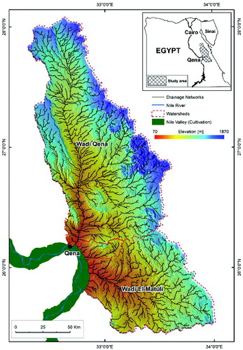
Interpretation of the geological map of Egypt (scale 1:2,000,000) revealed that the major rock succession in the study area is composed of the pre-Cambrian basement rocks (gabbro and granite) overlaid with thick sedimentary rocks (sand stone, shale, and calcareous rocks), ranging in age from the Cretaceous to Pliocene times. The sedimentary rocks are overlaid with loose and/or consolidated Quaternary deposits (alluvial, sand, gravels, and Nile deposits). Land reclamation is based mainly on the shallow aquifers within the Quaternary alluvial sediments (10–90 m depth) (Abdalla 2012; Hamdan 2013).

The mean annual rainfall is 2.5 [mm] in Qena that is mostly in the form of showers of short spells. It is characterized by high variable rainfall both interannually and on a monthly basis (Middleton & Thomas 1997) and it went without measurable precipitation for many years. However, one rain event over a short period may approach or exceed the mean values in the region that is often associated with thunderstorms mostly during spring and winter. The study area is characterized as well by great variability of temperature resulting in very hot summer and cold winter. The monthly average of air temperature ranges between 14.4°C and 33.1°C in January and July respectively, with an annual average of 25°C in Qena. The mean monthly evapotranspiration is relatively high 6.2 [mm/day].

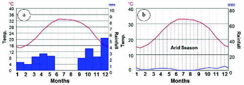
According to Köppen climate classification, the study area belongs to the hot dry desert (BWh) climate. To evaluate the local climatic condition that affects the land use and surface process, we implemented the rain-thermal quotient (Q) (Emberger 1954) that reads: (1) where P is the annual precipitation [mm], M mean maximum temperature of the hottest month, and m the mean minimum temperature of the coldest month. Accordingly, the study area belongs to hyper-arid regions since Q is significantly lower than 20 (Q = 0.28). Using the hygro-thermal climograms after Walter and Lieth (1967) reveals that precipitations are very low or absent throughout the year compared to the temperature curve (P < 2T) indicating also hyper-arid conditions as the dryness is predominant over the year (figure 2).

Figure 2. (a) Climograms show a combination of average monthly temperature and (b) total rainfall and length of the dry season after Walter-Leith.

Owing to the scanty rainfall throughout the year, floods occur infrequently in the study area (Qena). Rainfall is greatly variable over time and space along the entire drainage basin even during the heavy storm events. Therefore, floodwaters derivenormally from a part of the drainage basin, and both flood volumes and peaks are then influenced by the comparatively affected small parts and surface response. The historical background of flashfloods in the study area is shown in table 1.

Table 1. Historical flash floods in Qena.

Date	Rainfall [mm] in Qena	Affected villages/areas	Victims/damages
23 December 1955	6	Qena City	Destroyed many houses, roads and flooded cultivated lands
26 November 1968	Light	Klaheen Village	Displaced 2165 persons
		Shaykhiya Village	Displaced 94 persons
5 and 6 March 1975	2	Karm Omran, Al Ashraf Al Sharqiya Villages	Displaced 8 families
13 March 1975		El Hamydat Village	Displaced 68 persons
April 1975	0	Karm Omran Village	Displaced 289 persons
16 October 1979	7.8*	Hegaza Bahry Village	Displaced 2850 persons
May 1979	12	Hegaza Qebly Village
30 December 1980	1.1	Vast areas of the region	Destroyed 23 houses and 370 ha
April 1983	0	Alklahin Village and neighbours	Destroyed many houses, roads and flooded cultivated lands
April 1984	0	Khozam and Hegaza Villages	Killed 13 persons
20 April 1985	0.1	Wadi Banat Bary and neighbours	Destroyed Khozam Dam and killed 32 persons
8 October 1994	2*	Nag Salem, Alklahin, Hela, Hegaza, Abu Manaa, Abdel Qader Villages	Killed one person, displaced 6856 families, 1915 ha flooded, and destroyed the main highway (Qena-Safaga and Qeft- El Qusier).
2 November 1994	1.8
13 November 1997	0	Upper Egypt: Aswan, Sohag, Asyut, Minya, Qena	Killed 23 persons, thousands of hectares of land flooded and 260 houses destroyed
30 December 2010	8.9	Nag Salem and Attyat Bdhna Villages	Destroyed 9 houses, Qena-Safga highway and Cairo Aswan highway
28 January 2013	15	Alklahin and Karm Omran Villages	Broke down electricity and major roads for several hours, flooded cultivated lands

*Data reported by the weather station 624050 in Luxur.

3. Data and methods

In this study, we used different data types and methods of analysis (figure 3), which are summarized as follows:

Figure 3. Study scheme (modified after Moawad 2013).

3.1. ASTER GDEM data

ASTER (Advanced Spaceborne Thermal Emission and Reflection Radiometer) GDEM-2 is a product that is generated from a pair of ASTER Level-1A images. This Level-1A input includes bands-3N (nadir) and -3B (after viewing) from the visible near infra-red (NIR) telescope's along-track stereo data that is acquired in the spectral range of 0.78 to 0.86 μm. The absolute vertical accuracy of the GDEM-2 mean error is −0.20 meters on average with accuracy of 17 meters at the 95% confidence level, which is a significant improvement compared to the GDEM v1 mean error of −3.69 meters (Gesch et al. 2011). The number of voids and artefacts noted in GDEM1 were substantially reduced in GDEM2. ASTER GDEMs are generally expected to meet map accuracy standards for scales from 1:50.000 to 1:250.000 (http://idn.ceos.org). ASTER DEMs are available for download from NASA's EOS data archive and Japan's Ground Data System (https://wist.echo.nasa.gov).

The study area is extracted from four ASTER DEM images acquired on 17 October 2011 in GEOTIFF format. The images are projected using geographic Lat/Long, datum WGS84. Each image covers an area ∼60 km × 60 km with image dimension 2500 rows × 2500 columns. The input image resolution is 15 m although the output DEM resolution is 1 arc second (30 m). The cubic convolution method has been applied to the ASTER DEMs to acquire finer cell size of ∼15 m ground resolution. The technique performs sharpening edges of the topographic features and better stream network extractions (Moawad & Khidr 2011). This procedure takes into account the weighted neighbouring pixel values to change the spatial frequency of an image (Jensen 2005).

3.2. Satellite real-time rainfall data

The basic approach in this paper is to use the real-time satellite coverage for tracing the rainy storm on 28 January 2013, in particular. For that purpose, we collected a set of satellite data from 23 to 31 January, −5 and +3 days before and after the storm, respectively. The data were obtained from Hydrological Data and Information System (HYDIS) precipitation mapping server available at http://chrs.web.uci.edu/persiann/data.html. These real-time satellite images have led to the expansion of our understanding of storm dynamics.

The averaged six hours HYDIS data are produced from the Precipitation Estimation Remote Sensing Observation using Artificial Neural Networks (PERSIANN) system. It is designed and operated at the Center for Hydrometeorology and Remote Sensing (CHRS) at the University of California, Irvine, in collaboration with the International Hydrological Programme (IHP) of the United Nations Education Science and Cultural Organization (UNESCO). The PERSIANN algorithm provides global precipitation estimation using combined geostationary and low-orbital satellite imagery, e.g. NASA, NOAA, and DMSP low-altitude polar orbital satellites (TRMM, DMSPF-13, F-14, and F-15, NOAA-15, 716, 717) (Sorooshian et al. 2008). The data are available in ASCII format of 0.25° × 0.25° spatial resolution.

3.3. Adjustment of the satellite rainfall data

Uncertainty in satellite precipitation estimates can be highly variable due to many factors, such as retrieval technique, weather/climate regime, and rainfall type (Hsu & Sorooshian 2009). For that the bias of the satellite data needs to be adjusted. The standard errors of PERSIANN estimates in different regions are linearly related to the magnitude of the monthly average precipitation, with the slope of the relationship being related to spatio-temporal resolution. This relationship enables the generalization of PERSIANN, the error properties over the regions where gauge and/or radar observations are limited or missing. These may explain the presence of over- and under estimation(s) in the satellite rainfall data in comparison with the surface observed rainfall. In this study, we used in situ daily rainfall data obtained from five climatic stations from 28 to 30 January 2013 as reference data. We assumed that these data are much more reliable as they are directly measured at the surface. The in situ observed rainfall (R_obs) data differ from the satellite rainfall data (R_sat) in terms of scale and resolution since they are sparsely located and provide only point-scale measurement. However, the satellite rainfall data (R_sat) were extracted using explicit x and y coordinates of the observed rainfall (R_obs) data and some statistical variables (difference, mean, Stdv, R²) were inspected as shown in table 2.

Table 2. Statistical analysis, estimated rainfall and model efficiency.

Stations	Robs [mm]	Rsati [mm]	Diff.	Avg.	Std. (σ)	Resti [mm]	ME
Qena	15	5.94	9.06	10.47	4.53	13.12	0.95
Luxur	14.99	4.59	10.4	9.79	5.20	7.46	0.15
El Qusier	5.08	5.43	−0.35	5.26	0.18	10.75	−9.75
Alexandria	2.03	4	−1.97	3.02	0.99	5.59	0.45
Dabaa	0.76	0.95	−0.19	0.86	0.10	1.78	0.97
Arish	3.05	0.32	−2.73	1.69	1.37	2.21	0.95

We assumed that some variable of interest (y) can be driven by some other variable (x). Plotting the R_sat versus R_obs on a scatter diagram revealed two major peaks, which means that the polynomial function is the best fitting method between y and x rather than the linear function. Polynomial fitting curves of different orders were tested, of which, the second order was preferred as the best fitting based on data fluctuations (peak, trough) but reliability of the trend was not very high (R² = 0.49), nevertheless. Predicted values using linear, arithmetic, and polynomial functions of orders three and four were unrealistic. Then, R_sat was corrected based on the R_obs by implementing the regression analysis based on the following equation: (2) where is the estimated rainfall [mm] at a pixel i; and the satellite rainfall data [mm] at the same pixel i; and a and b are coefficients obtained from the polynomial fitting, which define the estimated rainfall as the polynomial curve of the second order fitting to the data. Accuracy of the estimations was performed using the following equation: (3) where is the model efficiency; in situ observed rainfall; averaged in situ rainfall; and n the number of observations. Values closer to 1 indicate the superior model performance (Mayer & Butler, 1993). Results of the model are shown in table 2. By this mean we adjusted the rainfall over the study area from 23 to 31 January 2013, to monitor the influences of flood processing, five days preceding the event and three days after its occurrence.

3.4. Hydrological modelling

The present study uses ArcGIS Hydro-model based on raster GIS tools to extract the drainage network. ArcGIS Hydro-model is a systematic framework specially designed for creating water resources geodatabases (Maidment 2002). In this study, the hydrological model was based on ASTER DEM (GDEM-2), which is a powerful tool to automatically extract hydrographs and to perform hydrological analysis, with both operational and quality advantages (Moawad & Khidr 2011; Moawad 2013). Drainage system extraction was done by determining the directions that water will flow out of each cell to its steepest down-slope neighbour (flow direction) relying on the 8D method (O’Callaghan & Mark 1984). Flow accumulation function was applied to tabulate for each cell the number of cells that will flow to it (Chang 2006) and cells of high-flow accumulation were used to identify the trunk channels.

First, the pour points of the main wadis were accurately determined from Google Earth by the explicit (x, y) coordinates. Next, different arbitrary threshold values were examined for delineating drainage networks (Martinez-Casasnovas & Stuiver 1998), of which a threshold value ≥150 cells has been found to provide a realistic density of drainage streams in the Eastern Desert of Egypt (Moawad & Khidr, 2011). The resulting streams likely correspond to a network obtained from traditional methods using topographic maps of scale 1:50,000 (Tarboton et al. 1991; Moawad 2008). Then, streams were extracted by assigning the flow accumulation layer to integer values ≥1 for a stream and no-data for background. After that, drainage networks were imported into Google Earth to visually verify the reliability of the output streams. Finally, streams were ordered according to Strahler (1957). For the purposes of data representation, major and trunk streams are only represented while the lower orders (i.e. orders first, second, and third) were excluded.

4. Morphometric analysis

The total drainage area is 23,300 km² (15,700 km² for wadi Qena and 7,600 km² for wadi El Matuli). The pattern of wadi Qena is commonly trellised and rectangular and clarifies the structural influences that resulted in parallel and sub-parallel streams specifically in the upstream area where the lower stream orders surprisingly descend from the mountains. The trunk stream itself flows from north to south generally, opposite to the general slope of the Egyptian land. In wadi El Matuli, the main pattern of the drainage network reveals dendritic like-pattern that dominates specifically the upstream area.

The length of the basins differs from 207.5 km for wadi Qena and 126.7 km for wadi El Matuli, measured along the trunk streams. Wadi Qena is of the eighth order with a total (∑N) 19,989 streams and wadi El Matuli attains the seventh order with a total 10,071 streams. Basin relief differs from 1807 m and 935 m and basin gradients differ from 8.4 and 7.4 m/km in the same order. Drainage density (D_d) is poor (1.3 km/km²), circularity and elongation ratios after Miller (1953) and Schumm (1956), respectively, reveal fern leaf-like shape generally. These characteristics increase the concentration time and decrease flood magnitude and volume. Long concentration time implies more opportunities for water infiltration as well (Pallard et al. 2009).

5. Antecedent and associated weather conditions

Egypt, the Red Sea, and NW Saudi Arabia were battered by a thunderstorm from 28 to 30 January 2013. The storm led to severe weather event with potentially life-threatening. The antecedent weather conditions can be traced and summarized based on satellite real-time rainfall images, Meteosat infrared images, and weather reports as follows (figure 4):

Figure 4. Daily development of storms over the Sahara from 23 to 28 January 2013.

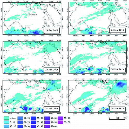
1. 23 January 2013: A storm originated from the tropical (Gulf of Guinea) and sup-tropical Western Africa and passed through the central Sahara toward the north eastern Mediterranean. The north western coast of Egypt was influenced by shower rain (>0.5 [mm]).

2. 24 January: The storm developed as a branch from the sub-tropical Western Africa, carrying humid air from the sub-tropical Atlantic Ocean. The storm trend was generally SW-NE and passed through central Sahara to the Levant, where it forced the cold air to plunge southward from southern Europe. It influenced Northern and Middle Egypt, Northern Sinai Peninsula, Israel, Jordan, Lebanon, Syria, and Iraq. The storm led to increased temperature over Cairo (23°C) and Upper Egypt (Aswan 31°C) during the daytime, while it was relatively cold at night (Cairo 12°C and Aswan 15°C).

3. 25–26 January: The same conditions prevailed with the accumulation of low and middle clouds accompanied with heavy rain over Upper Egypt, South Sinai, and the Red Sea.

4. 27 January: The weather was generally warm during the daytime and cold during the night as the maximum and minimum temperatures significantly decreased (Cairo 19°–11°C; Luxor 25°–12°C; Aswan 27°–14°C). The accumulation of low and middle clouds was accompanied with heavy rain over Upper Egypt, South Sinai, and the Red Sea.

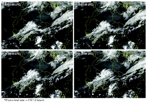
5. 28–29 January: The general weather condition was unstable as the subtropical jet stream passing through the Gulf of Guinea and Central Africa invaded Egypt from SW; meanwhile the upper-air cold low pressure has plunged southward from Southern Europe, wandering over NW Egypt and extending up to Upper Egypt. On the other hand, the Sudanese Monsoon (inverted v shape) dominated over the Red Sea. As a result, the maximum and minimum temperatures were suddenly and significantly decreased owing to the cold wind of high speeds (Cairo 16°–7°C; Qena 17°–10°C; Luxor 18°–12°C) and low and middle clouds covered wide areas of Middle, Upper, and Eastern Egypt as well. During the early hours of Monday, 28 January (∼1:45 am, Cairo local time = 27 January 23:45 pm UTC), a rainy thunderstorm battered Qena, Upper Egypt, and lasted about two hours (∼4:00 am local time = 2 am UTC) (figure 5). The rain was relatively heavy over Upper Egypt, Eastern Desert, Red Sea, South Sinai and light over Northern Egypt. The duration of the rain storm was about two hours continual. It resulted in weak to medium flash floods in South Sinai, Eastern Desert, Qena, and Safag and El Qusier on the coast of the Red Sea.

   Figure 5. Infrared Eumetsat images show 6-hours development of the jet streams over the Sahara from 27 January 2012 (23:00 pm UTC) to 28 January 2013 (02:00 am UTC).

   

6. 30 January: The storm moved to northern Saudi Arabia, Jordan, Iraq, Kuwait, and north-western Iran.

6. Rainfall analysis

Cumulative rain map was processed by adding the daily rainfall from 23 to 30 January 2013. Figure 6 shows that the maximum rain was about 13.5 [mm] that was mainly concentrated on the north eastern part of wadi Qena. The total cumulative rain ∑R_cum was estimated as 32 × 10⁶ [mm] and 3.6 × 10⁶ [mm] for wadis Qena and El Matuli, respectively. Rain volume for a given cell in the spatial model was then estimated as (Moawad 2013): (4)

Figure 6. (a) Cumulative rainfall (R_cum) [mm] and (b) volume of rainfall (R_vol) [m³] from 23 to 30 January 2013.

where is the rain volume for a given pixel (i) [m³], cumulative rainfall [mm], cell size [m²]. Accordingly, the study area received a total rain volume (∑R_vol) of approx. 88.9 × 10⁹ [m³], divided as 79.9 × 10⁹ [m³] (89.8%) from wadi Qena and 9 × 10⁹ [m³] (10.2%) from wadi El Matuli and other small drainage basins.

The intensity of rain was calculated to oversee the rain strength during 28 January for each six hours using the following equation (Flood Control Center 2003): (5) where is the rain intensity for a given pixel (i), six-hours rainfall within a pixel i, D storm duration in minutes. The results reveal that the strength of rain varied in time and space between 0.14 and 1.48 [mm hr⁻¹], generally, and the majority fell at light intensity (<2.5 [mm hr⁻¹]). Based on experiences from the Sahara and the daily weather reports obtained from the Egyptian Meteorological Authority, rainfall falls over a shorter time period mostly, two hours in this case, but the radar systems assemble the images only every six hours (Moawad 2013). Therefore, we calculated the actual rain strength over two hours of storm duration from 2:00 to 4:00 am (Cairo local time). It reveals light to relatively moderate intensity that ranges between 0.29–2.97 (figure 7); however, it was associated with the vast majority of flash floods simply because it brought large amounts of rainfall water in a short time, mainly from the central part of wadi Qena (figure 6).

Figure 7. (a) Rain strength for 6 hours of storm duration and (b) actual rain strength for 2 hours of storm duration on 28 January 06:00 am [mm hr⁻¹].

7. Hydrological soil group and hydrological conditions

From the east, the wadis drain of the basement rocks of the Red Sea Mountains that are mostly impervious. Except that, the major part of the soil is mainly sandy soil and gravelly lithosols of the desert plains with dissected limestone rocky hills and escarpments of different rocks. Trunk and major streams are filled with gravelly loamy sands (torrifluvents) and calcaric regosols developed from limey substrate. The lower part is composed of gravel and gravelly sand soil of alluvial fans, outwash plains, Nile Terraces and Nile flood plain. Flora of the wadis is generally poor and represents a thin cover (Zahran & Willis 2009). The alluvial fans are widely reclaimed for agricultural activities and dispersed settlements of farmers.

However, geological and soil maps of Egypt (scales 1:2,000,000) were used to determine the hydrological soil group (HSG) and to identify the initial losses based on the curve number method (CN) developed by the United States Department of Agriculture, Soil Conservation Service (SCS 1985). The empirical CN is a function of the antecedent moisture condition (AMC), land use, hydrological condition, and hydrological soil type (SCS 1985). Three HSGs were identified in the study area as follows (figure 8):

Figure 8. Hydrological soil groups (HSG), adjusted curve number (CN _I) [unitless] and surface infiltration.

1. Alluvial: well drained with low runoff potential and high infiltration rate (type A: infiltration rate >7.5 [mm h⁻¹], initial CN_II: 68).

2. Sandy soils: moderate infiltration rates, fine to coarse textures with moderate rate of water transmission (type B: infiltration rate 3.75–7.5 [mm h⁻¹], initial CN_II: 79).

3. Impervious surfaces: surfaces that have high runoff potential and infiltration capacity are extremely limited. They are composed of massif basement rocks and dissected limestone. Such surfaces have relative low infiltration rates (type D: infiltration rate 0–1.25 [mm h⁻¹], initial CN_II: 98).

The initial Runoff Curve Number (CN_II) was derived from the published lookup tables by the SCS (1986). The final values were adjusted based on the AMC that is a function of the total rainfall in the five days preceding a storm. Accordingly, the AMC was assumed to be generally low (AMC-I = dry condition) since the preceding rain was very low (<5 [mm]). Hydrologic conditions (cover type) were classified as natural desert landscape and desert shrub (poor coverage). Therefore, CN_II was adjusted as follows (Chow et al. 2002): (6) where is the curve number for dry condition (AMC-I) and the initial curve number for normal condition (AMC-II). Accordingly, the values are 47, 61, and 95 for the hydrological groups A, B, and D, respectively. The higher the CN value the higher the runoff potential, generally.

8. Flow analysis

In this study, the hydrological parameters that influence the water runoff were included in the empirical black-box model (BBM) based on a single regression relationship (Davie 2008) to predict stream runoff from rainfall depending on the CN approach. This model is commonly used in the United States in areas lacking good coverage by rain gauges and/or areas having poor runoff records, a situation like that encountered in the study area, and for humid, semi-arid, and arid conditions (SCS 1986). It is also widely applied to several wadis in the Eastern Desert of Egypt and Sinai by Gheith and Sultan (2001, 2002), Foody et al. (2004), Moawad (2008), Moawad and Khidr (2011) and Moawad (2012, 2013). Surface runoff (Q_surf) was estimated as follows: (7) where is the surface runoff [mm] for a given pixel; storm precipitation total for the same pixel [mm], this was compensated by the cumulative rainfall ; and the potential retention parameter or surface storage after runoff begins [mm] that is a function of an empirical CN coefficient where: (8) CN_I values were weighted in proportion to cell size to compute the composite curve number for each subbasin. Eventually, the total surface runoff (∑Q_sur) was estimated as 26 × 10⁶ [mm] and 4.7 × 10⁵ [mm] for wadis Qena and EL Matuli, respectively. Moreover, runoff volume () for a given cell was estimated as: (9) where is obtained from equation 7 [mm], cell size is in units of ground distance [m²] and (Q_vol) in cubic meters (figure 9). Accordingly, the total runoff volumes (∑Q_vol) were estimated as 65 × 10⁶ [m³] and 1.2 × 10⁶ [m³] for wadis Qena and EL Matuli, respectively, and the total transmission losses (∑T_los) were estimated as 6 × 10⁶ [mm] and 3.1 × 10⁶ [mm] in the same order (table 3).

Table 3. Hydrological estimations.

Wadi	Area [km^2]	∑Rcum [mm]	∑ Rvol [m^3]	∑Qsur [mm]	∑Qvol [m^3]	∑Tlos [mm]
Qena	15,700	32 × 10^6	79.9 × 10^9	26 × 10^6	65 × 10^6	6 × 10^6
El Matuli	7600	3.6 × 10^6	9 × 10^9	4.7 × 10^5	1.2 × 10^6	3.1 × 10^6
Total	23,300	35.6 × 10^6	88.9 × 10^9	26.5 × 10^6	66.2 × 10^6	9.1 × 10^6

Figure 9. (a) Estimated surface runoff (Q_sur) [mm] and (b) runoff volume (Q_vol) [m³].

9. Results and discussion

Quantified understanding of flood hydrology and risk management in the Sahara is severely hampered by the lack of hydrological data on a spatio-temporal scale. As a result, there are inconsistency and ambiguities in the flood protection and water management plans. As, rainfall and surface response are the cornerstones of the flood process, the present study is based primarily on the integration of remote sensing and GIS techniques to estimate the surface runoff in Qena territory, Upper Egypt, using the empirical curve number method (CN) (SCS 1985). The basic approach in this paper is to use a set of the real-time satellite rainfall coverage (HYDIS) to avoid the lack of rainfall data and to monitor the development of the storm that occurred on 28 January 2013, which led to surface runoff in Eastern Qena and its neighbours. Interpretation of the satellite images revealed that the general weather condition was instable and the area was under the influence of the subtropical jet stream that passed through the subtropical Western and Central Africa. This was accompanied with an upper-air cold low pressure that plunged southward from Southern Europe. Meanwhile, the Sudanese Monsoon dominated over the Red Sea Region. These resulted in a rainy thunderstorm that battered many parts of Egypt (i.e. Upper Egypt, Eastern Desert, Red Sea, and South Sinai) and lasted about two hours.

As the standard error of the satellite derived rainfall data can be highly variable due to retrieval technique, weather/climate regime and rainfall type (Hsu & Sorooshian 2009), we adjusted the satellite rainfall date using in situ observed daily rainfall obtained from five climatic stations from 28 to 30 January 2013 as reference data. We assumed that the in situ observed rainfall data (R_obs) are much more reliable than the satellite derived rainfall (R_sat) as they are directly measured at the surface, although they differ from the satellite data in terms of scale and ground resolution. We supposed that the relation between the two data types can be estimated using statistical modelling and analyses. We found that the polynomial function of the second order is the best fitting method based on data fluctuations but reliability of the trend was not very high (R ² = 0.49), nevertheless. However, calculation of model efficiency (EM) revealed that the method reduces over- and underestimations in the satellite data in comparison with the surface observed rainfall and accuracy of the estimated rainfall (R_est) that are in the acceptable range when they are applicable to small- and/or mesoscale drainage area (∼300 km in the horizontal extent). We noted that this method of statistical analysis is not appropriate for large and/or regional scales as the uncertainty propagates and the estimated values (R_est) become unrealistic in this case. By this mean, we revealed that the study area received a total precipitation (∑R_cum) of ∼35.6 × 10⁶ [mm] and a total rain volume (∑R_vol) of ∼88.9 × 10⁹ [m³] mainly from wadi Qena 79.9 × 10⁹ [m³] (89.8%) and 9 × 10⁹ [m³] (10.2%) from wadi El Matuli. The majority of the rain fell at light intensity (<2.5 [mm hr⁻¹]) and the actual rain strength was calculated over two hours of storm duration based on the daily weather report as 0.29–2.97 [mm hr⁻¹] from 2:00 to 4:00 am (Cairo local time) on 28 January 2013. This was the time associated with the vast majority of flash floods.

On the other hand, the hydro-morphometric parameters were determined from the hydrological model based on ASTER DEM (GDEM-2) and quality of the extracted drainage streams were inspected on Google Earth. Three HSGs were determined from the soil map of Egypt with the aid of the geological map (scale 1:2,000,000) namely alluvial, sandy soil, and impervious surfaces. The initial curve numbers (CN_II) of the HSG were then extracted from the lookup tables developed by the United States Department of Agriculture, Soil Conservation Service (SCS 1985) as 68, 79, and 98, respectively. Then, we adjusted the CN_II to CN_I (dry condition) based on the AMC that is a function of the total rainfall in the five days preceding a storm (<5 [mm]) as 47, 61, and 95 in the same order. Then, the total surface runoff (∑Q_sur) was estimated as 26.5 × 10⁶ [mm], which represents 74.4% of the total precipitation (∑R_cum). The total runoff volumes (∑Q_vol) were estimated as 66.2 × 10⁶ [m³] and the estimated total surface transmission losses (∑T_los) were about 9.1 × 10⁶ [mm], which represents about one-fourth of the total precipitation.

Most of the losses are due to water penetration into the surface of soil through infiltration process and fractures, except very few that were intercepted by a plant and underwent evapotranspiration since the vegetation cover is generally poor. The low infiltration capacity of the basement rocks and limestone creates substantial runoff over the Red Sea Mountains even from low precipitation events. The dry alluvial deposits with their high infiltration capacities and the large and extensive drainage networks create substantial opportunities for alluvial aquifer recharge through transmission losses (Milewski et al. 2009).

The accuracy of the model parameters is very crucial. Parameters used in this study could be divided into two types: physical parameters, which were generated directly from DEM, geology, and soil maps; and calibrated parameter, which was derived from rainfall data. Although the calibration optimizes the satellite rainfall data in comparison with the surface observed rainfall, the upstream mountainous area(s) suffers from an absence of gauged measurements that prevents the accurate calibration of the final output. Therefore, accuracy and reliability of our model were tested in comparison with field observations reported from surrounding watersheds during 1994 and 2010 events (see table 1) and other previous literatures (Naim 1995; Gheith & Sultan 2002; Milewski et al. 2009; Moawad 2013). The results are very reasonable as the watersheds respond realistically to the rainfall, which revealed a random spatial distribution of varying magnitude from 1994 to 2013. Thus, we deduced that the total surface runoff (∑Q_sur) and so the flood magnitude was generally low and proportional to the total precipitation (∑R_cum) in comparison with other estimates (e.g. Naim 1995; Gheith and Sultan 2002; Milewski et al. 2009; Moawad 2013). This resulted in limited influences, such as destruction of some infrastructure in Qena but no fatalities were involved, nevertheless. Most of the running water was contained by El Sail Canal to be poured into the Nile River.

It is expected that the application of the proposed method in this study will be helpful for the understanding and quantification of flood hydrology and risk management in the arid and hyper-arid regions, generally. It will also contribute to better risk action plan and water management specifically in the Sahara since the demand for freshwater is increasing significantly due to population growth and economic development.

Acknowledgements

The authors would like to thank the anonymous reviewers for their valuable comments and suggestions to improve the manuscript.

References

- Abdalla F. 2012. Mapping of groundwater prospective zones using remote sensing and GIS techniques: a case study from the Central Eastern Desert, Egypt. J Afr Sci. 70:8–17.
- Ashour MM. 2002. Flashfloods in Egypt (a case study of Drunka village – Upper Egypt). Bull Soc Gèog Ègypte. 75:101–114.
- Bbc Archive, Dozens killed in Morocco floods. Available from: http://news.bbc.co.uk/2/hi/africa/2511817.stm
- Chang KT. 2006. Introduction to geographic information systems. 3rd ed. Singapore: McGraw Hill; p. 343.
- Chow VT, Maidment DK, Mays LW. 2002. Applied hydrology. New York: McGraw-Hill Book Company; p. 572.
- Davie T. 2008. Fundamentals of hydrology. London: Routledge; p. 200.
- Dolman AJ, Gash JHC, Goutorbe J-P, Kerr Y, Lebel T, Prince SD, Stricker JNM. 1997. The role of the land surface in Sahelian climate: HAPEX-Sahel results and future research needs. J Hydrology. 188–189:1067–1079.
- Emberger L. 1954. Une classification biogéographique des climats. Rec Trav Lab Bot Géol Zool Univ Montp Série Bot. 7:3–43.
- Flood Control Center. 2003. San Diego county hydrology manual. San Diego: San Diego County Flood Control Advisory Commission; p. 322.
- Foody GM, Ghoneim EM, Arnell NW. 2004. Predicting locations sensitive to flash flooding in an arid environment. J Hydrology. 292:48–58.
- Gesch D, Oimoen M, Zhang Z, Danielson J, Meyer D. 2011. Validation of the ASTER Global Digital Elevation Model (GDEM) Version 2 over the Conterminous United States. Sioux Falls, South Dakota, USA: U.S. Geological Survey, Earth Resources Observation Science (EROS) Center.
- Gheith HM, Sultan MI. 2001. Assessment of the renewable groundwater resources of Wadi El-Arish, Sinai, Egypt: modelling, remote sensing and GIS applications. Proceedings of a symposium held at Santa Fe; April 2000; New Mexico: IAHS Publ. no. 267.
- Gheith HM, Sultan MI. 2002. Construction of a hydrologic model for estimating wadi runoff and groundwater recharge in the Eastern Desert, Egypt. J Hydrology. 263:36–55.
- Hamdan AM. 2013. Hydrogeological and hydrochemical assessment of the Quaternary Aquifer South Qena City, Upper Egypt. Earth Sci Res. 2:11–22.
- Heidari A, Saghafian B, Maknoon R. 2006. Assessment of flood forecasting lead time based on generalized likelihood uncertainty estimation approach. Stoch Environ Res Risk Assess. 20:363–380.
- Hsu L, Sorooshian S. 2009. Satellite-based precipitation measurement using PERSIANN system. In: Sorooshian S, Hsu L, Coppola E, Tomassetti B, Verdecchia M, Visconti G, editors. Hydrological modelling and the water cycle. New York: Springer; p. 27–48.
- Irin. 2013. Preparing for floods in West Africa. Available from: http://reliefweb.int/report/nigeria/-preparing-floods-west-africa.
- Jensen J. 2005. Introductory digital image processing. 3rd ed. Upper Saddle River: Prentice Hall; p. 526.
- Karmakar S, Simonovic SP, Peck A, Black J. 2010. An information system for risk-vulnerability assessment to flood. J Geogr Inf Syst. 2:129–146.
- Kenyon P. 2007. Climate connections: Algeria vs. the Sahara, NPR's climate connections series with National Geographic. Available from: www.npr.org/templates/story/story.php?storyId=12903558">http://www.npr.org/templates/story/story.php?storyId=12903558">www.npr.org/templates/story/story.php?storyId=12903558.
- Khidr MM. 1997. The main geomorphological hazards in Egypt (in Arabic). MSc thesis. Cairo: Department of Geography, Faculty of Arts, Ain Shams University; p. 513.
- Laity JE. 2008. Deserts and desert environments. Oxford, UK: Wiley-Blackwell; p. 360.
- Maidment DR. 2002. Arc hydro: GIS for water resources. California: ESRI; p. 222.
- Martinez-Casasnovas JA, Stuiver HJ. 1998. Automatic delineation of drainage networks and elementary catchments from digital elevation models. ITC J. 3/4:198–208.
- Mayer DG, Butler DG. 1993. Statistical validations. Ecol Modell. 68:21–32.
- Middleton NJ, Thomas DSG, editors. 1997. World atlas of desertification. 2nd ed. London: UNEP; p. 182.
- Milewski A, Sultan M, Yan E, Becker R, Abdeldayem A, Soliman F, Abdel Gelil K. 2009. A remote sensing solution for estimating runoff and recharge in arid environments. J Hydrology. 373:1–14.
- Miller VC. 1953. A quantitative geomorphic study of basin characteristics in the Clinch Mountain area. Virginia and Tennessee, Project NR 389-042, Tec. Rept. 3. New York: Columbia University, Department of Geology, ONR, Geography Branch; p. 51.
- Moawad BM. 2008. Applications of remote sensing and geographic information systems in geomorphological studies: Safaga- El Quseir area, Red Sea, Egypt as an example. Saarbrücken: VDM Verlag Dr. Müller; p. 282.
- Moawad BM. 2012. Predicting and analyzing flash floods of ungauged small-scale drainage basins in the Eastern Desert of Egypt. J Geomatics, Indian Soc Geomatics. 6:23–30.
- Moawad BM. 2013. Analysis of the flash flood occurred on 18 January 2010 in wadi El Arish, Egypt (a case study). Geomatics, Nat Hazards Risk. 4(3):254–274.
- Moawad BM, Khidr MM. 2011. A GIS and RS based approach for modeling ungauged small-scale catchments in Mersa Alam. Bull Soc Gèog Ègypte. 84:117–140.
- Naim G. 1995. Floods of Upper Egypt governorates. Cairo: Egyptian Geological Survey and Mining Authority.
- Nasa, Earth Observatory, Torrential rains bring floods to Western Sahara. Available from: http://earth-observatory.nasa.gov/Newsroom/view.php?id=29032.
- Nfrag. 2008. Flood risk management in Australia. Aust J Emerg Manag. 23(4):21–27.
- O’callaghan JF, Mark DM. 1984. The extraction of drainage networks from digital elevation data. Comput Vis, Graphics Image Process. 28:323–344.
- Ocha. 2012. Mali Complex Emergency Situation Report No. 15. 11 September 2012. Available from: http://www.un.org/maintenance/.
- Pallard B, Castellarin A, Montanari A. 2009. A look at the links between drainage density and flood statistics. Hydrol Earth Syst Sci. 13:1019–1029.
- Reid I, Frostick LE. 1997. Channel form, flows and sediments in deserts. In: Thomas DSG, editor. Arid zone geomorphology: process, form and change in drylands. New York: John Wiley; p. 205–229.
- Reid I, Powell DM, Laronne JB, Garcia C. 1994. Flash floods in desert rivers: studying the unexpected. Eos, Trans Am Geophysical Union. 75–39:452.
- Schumm SA. 1956. Evolution of drainage systems and slopes in badlands at Perth Amboy. N J Geol Soc Amer Bull. 67:597–646.
- Scs (US SOIL CONSERVATION SERVICE). 1985. National Engineering Handbook. Washington, DC: US Department of Agriculture, US Government Printing Office.
- Scs (US Soil Conservation Service). 1986. Urban hydrology for small watersheds. Technical Report 55 Springfield, VA: USDA.
- Sene K. 2013. Flash floods: forecasting and warning. Dordrecht, Germany: Springer; p. 395.
- Sorooshian SK, Hsu L, Imam B, Hong Y. 2008. Global precipitation estimation from satellite image using artificial neural networks. In: Wheater H, Sorooshian S, Sharma KD, editors. Hydrological Modelling in Arid and Semi-Arid Areas. Cambridge: Cambridge University Press; p. 21–27.
- Strahler AN. 1957. Quantitative analysis of watershed geomorphology. Am Geophys Union Trans. 38:913–920.
- Takeuchi K. 2006. ICHARM calls for an alliance for localism to manage the risk of water-related disasters. In: Tchiguirinskaia I, Thein KNN, Hubert P, editors. Frontiers in flood research. the Netherlands: IAHS Press; p. 197–208.
- Tarboton DG, Bras RL, Rodriguez-Iturbe I. 1991. On the extraction of channel networks from digital elevation data. Hydrol Process. 5:81–100.
- Trommer JT, Loper JE, Hammett KM. 1996. Evaluation and modification of five techniques for estimating stormwater runoff for watersheds in West-Central Florida. U.S. Geological Survey, water-resources investigation report 96-4158. Florida: Tallahassee;p. 41.
- Walter H, Lieth H. 1967. Klimadiagramm-Weltatlas. Jena, Germany: VEB Gustav Fischer Verlag; p. 506.
- Warner TT. 2004. Desert meteorology. Edinburgh: Cambridge university press; p. 612.
- Zahran MA, Willis AJ. 2009. The Vegetation of Egypt. 2nd ed. New York: Springer; p. 237.