A stochastic model for earthquake slip distribution of large events

Abstract

This paper presents a stochastic model to simulate spatial distribution of slip on the rupture plane for large earthquakes (M_w >7). A total of 45 slip models coming from the past 33 large events are examined to develop the model. The model has been developed in two stages. In the first stage, effective rupture dimensions are derived from the data. Empirical relations to predict the rupture dimensions, mean and standard deviation of the slip, the size of asperities and their location from the hypocentre from the seismic moment are developed. In the second stage, the slip is modelled as a homogeneous random field. Important properties of the slip field such as correlation length have been estimated for the slip models. The developed model can be used to simulate ground motion for large events.

1. Introduction

Large-magnitude earthquakes (M_w > 7) occur frequently in active regions like Himalaya and northeast India. Even in the Indian shield, Gujarat region also experiences such large events. Due to their intensity and the geographical extent of the damage, large earthquakes pose the highest risk to the society. The 2001 Kutch earthquake (M_w = 7.7) caused severe fatalities and affected the economy of the Gujarat region. Recently, Raghukanth (2011) developed the earthquake catalogue for India and ranked the 48 urban agglomerations in India based on seismicity. The maximum possible magnitude in a control region of radius 300 km around the 24 urban agglomerations lies in between M_w = 7.1 and M_w = 8.7. This necessitates the estimation of the seismic input (design ground motion) in an accurate fashion for such large events to reduce the damages to structures. Cases where the recorded strong motion data are not available, the source mechanism models where in the earthquake slip distribution and medium properties can be modelled analytically are preferred to simulate ground motion for such large events. These models require the earthquake forces to be specified in terms of spatial distribution of slip on the rupture plane. Hartzell et al. (1999) and Raghukanth and Iyengar (2009) have demonstrated that surface level ground motions can be computed for an Earth medium for a given slip distribution on the rupture plane. These models provide reliable ground motion predictions if the fault and its slip distribution are known. Specifying the slip distribution on the rupture plane for future events is the most challenging problem in mechanistic models. To address this issue, there have been efforts to obtain spatial distribution of slip on the rupture plane by inverting ground motion records of the past earthquakes (Hartzell & Heaton 1983; Hartzell & Liu 1995; Ji et al. 2002; Raghukanth & Iyengar 2008). Several such finite slip models are available in various journals and research reports. The obtained slip distribution of past events exhibit higher complexity which can be modelled by stochastic approaches only. These techniques require very few parameters to characterize the slip field. Much effort has been made by the previous investigators in this direction (Somerville et al. 1999; Mai & Beroza 2002; Lavallée et al. 2006; Raghukanth & Iyengar 2009; Raghukanth 2010). Without going into the details regarding time-dependent stresses on the fault plane, few parameters have been identified from the slip distribution of past events. The slip distribution is modelled as a random field with a specified power spectral density (PSD). A total of 15 slip distributions with the magnitude of the events ranging from 5.66 to 7.22 have been analysed by Somerville et al. (1999). The total number of large events included in the database is two. Mai and Beroza's (2002) slip database includes 11 large events. This puts a serious limitation on the random field model developed by the previous investigators for simulating slip distribution for large events. Due to advances in instrumentation, several large events have been recorded by the broadband instruments operating around the world. These data have been processed and slip models for 45 large events are available in the literature. Since large events are of concern to engineers, it would be interesting to examine these slip distributions. In this paper, stochastic characterization of slip distribution is explicitly developed for large events. Important properties of the random field are estimated from the PSD of slip distribution. Empirical equations for estimating the slip field from magnitude are developed in this paper.

2. Slip database of large events

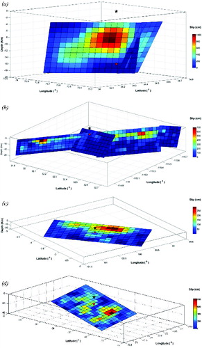
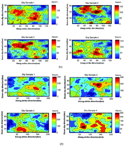
Inversion for earthquake sources is fundamental to understand the mechanics of earthquakes. The extracted slip models can be used to understand the damages in the epicentral region. Much effort has been made by seismologists in developing methods to extract slip distribution on the rupture plane from ground motion records. After the occurrence of a large event, the Incorporated Research Institutions for Seismology data management centre reports the broadband velocity data recorded by the Global Seismic Network (GSN). The preliminary earthquake slip distribution is determined from this data by several research groups. In case of local strong motion data, global positioning system and ground deformation measurements become available, these records are combined with the GSN data to obtain the spatial distribution of slip on the rupture plane. Several such slip maps for large events are available in the published literature. In this study, the source models of large events, reported by Chen Ji (http://www.geol.ucsb.edu/faculty/ji/) and tectonics observatory, California Institute of Technology (http://www.tectonics.caltech.edu/), are used to develop the model. The methodology for obtaining the rupture models is based on Ji et al. (2002), and is uniform for all the events. The compiled database from these two website consists of 45 rupture models coming from 33 earthquakes in the magnitude range of M_w 7–9.15 from various seismic zones in the world. These slip maps have been derived by the inversion of low-pass filtered ground motion data. The location of the epicentre, average slip, total seismic moment, faulting mechanism and dimensions of the fault plane of the 45 slip models are reported in tables 1 and 2. The slip database consists of 36 thrust events, 2 normal faulting mechanism and 7 strike-slip earthquakes. The epicentres of these large events along with plate boundaries as reported by Bird (2003) are shown in figure 1. Slip fields of some large earthquakes are shown in figure 2(a)–(d). It can be observed that the slip distributions exhibit high complexity which cannot be modelled through simple mathematical functions. Although the slip is continuous, the fault geometry for Kashmir and Mexico events is not planar. The source model of Mexico event consists of slip distribution on four planes, whereas Kashmir event consists of two rupture planes.

Table 1. Slip models used in this study.

S. no.	Location	Date (m/d/yy)	Latitude (°)	Longitude (°)	Mech (RV/N/SS)	Mw	M0 (Nm)	Ref.
1	Kuril Islands	10/04/94	43.77	147.32	RV	8.36	3.89E+021	1
2	Chile	07/30/95	−23.34	−70.29	RV	8.14	1.82E+021	1
3	Kuril Islands	12/03/95	44.66	149.30	RV	7.81	5.82E+020	1
4	New Britian Region	11/17/00	−05.50	151.78	RV	7.5	2.00E+020	1
5	Bhuj, India	01/26/01	23.42	70.23	RV	7.6	2.82E+020	2
6	Peru	06/23/01	−16.26	−73.64	RV	8.4	4.47E+021	1
7	North Sumatra	03/28/05	02.09	97.11	RV	8.68	1.17E+022	1
8		03/28/05	02.09	97.11	RV	8.5	6.31E+021	2
9	Northern California	06/15/05	41.29	−125.95	SS	7.2	7.10E+019	2
10	India	07/24/05	07.92	92.19	SS	7.25	8.40E+019	1
11	Honshu, Japan	08/16/05	38.28	142.04	RV	7.19	6.80E+019	1
12	Kashmir, Pakistan	10/08/05	34.54	73.59	RV	7.6	2.82E+020	2
13		10/08/05	34.54	73.59	RV	7.64	3.24E+020	1
14	Southern Java, Indonesia	07/17/06	−09.28	107.42	RV	7.9	7.94E+020	2
15	Kuril Islands	11/15/06	46.59	153.27	RV	8.3	3.16E+021	2
16	Kuril Islands	01/13/07	46.24	154.52	N	8.1	1.59E+021	1
17		01/13/07	46.24	154.52	N	8.1	1.59E+021	2
18	Solomon Islands	04/01/07	−08.47	157.04	RV	8.1	1.59E+021	1
19	Pisco, Peru	08/15/07	−13.39	−76.60	RV	8	1.12E+021	2
20	PagaiIsland, Indonesia	09/12/07	−02.62	100.84	RV	7.9	7.94E+020	2
21	Benkulu, Indonesia	09/12/07	−04.44	101.37	RV	8.5	4.47E+021	2
22		09/12/07	−04.52	101.38	RV	8.5	4.47E+021	1
23	Kepulauan	09/12/07	−02.62	100.84	RV	7.94	9.12E+020	1
24	Antofagasta, Chile	11/14/07	−22.25	−69.89	RV	7.81	5.82E+020	1
25		11/14/07	−22.25	−69.89	RV	7.78	3.98E+020	2
26	Simeulue, Indonesia	02/20/08	02.77	95.96	RV	7.4	1.41E+020	2
27	Tibet, China	03/20/08	35.49	81.47	N	7.14	5.80E+019	1
28	East Sichuan, China	05/12/08	31.00	103.32	SS	7.9	7.94E+020	2
29		05/12/08	31.00	103.32	RV	7.97	1.01E+021	1
30	Sulawesi, Indonesia	11/16/08	01.27	122.1	RV	7.3	1.00E+020	2
31	Padang, Indonesia	09/30/09	−00.72	99.87	SS	7.6	2.82E+020	2
32		09/30/09	−00.72	99.87	RV	7.6	2.82E+020	2
33	Vanuatu Islands	10/07/09	−13.05	166.18	RV	7.6	2.82E+020	2
34	Haiti	01/12/10	18.44	−72.57	SS	7	3.50E+019	2
35	Maule, Chile	02/27/10	−36.12	−72.90	RV	8.9	2.51E+022	1
36		02/27/10	−35.84	−72.72	RV	8.8	1.78E+022	2
37	El Mayor-Cucapah, Mexico	04/04/10	32.30	−115.28	SS	7.2	7.10E+019	2
38	Kepulauan, Indonesia	10/25/10	−3.480	100.12	RV	7.82	6.03E+020	1
39	Honshu, Japan	03/09/11	38.44	142.84	RV	7.4	1.41E+020	1
40	Honshu, Japan	03/11/11	38.32	142.34	RV	9.1	5.01E+022	1
41		03/11/11	38.32	142.34	RV	9.1	5.01E+022	1
42		03/11/11	38.10	142.86	RV	9.1	5.01E+022	1
43		03/11/11	38.10	142.86	RV	9.1	5.01E+022	1
44		03/11/11	38.10	142.80	RV	9	3.55E+022	2
45	Turkey	10/23/11	38.72	43.51	RV	7.13	5.60E+019	1

Note: 1: www.geol.ucsb.edu; 2: www.tectonics.caltech.edu; Faulting mechanism: RV – reverse, SS – strike slip, N –normal.

Table 2. Source dimensions and orientation of the fault plane.

	Length, L	Width, W	Mean slip, <D>	Subfault size, dx	Subfault Size, dz
S. no.	(Km)	(Km)	(cm)	(Km)	(Km)	Strike (°)	Dip (°)	Rake (°)	Area (1.0E+05* sq.km)
1	255	121	234.87	15	11	54	76	123.4	0.309
2	240	156	96.32	15	13	4	18	90.9	0.374
3	168	112	67.57	14	14	226	18	100.3	0.188
4	168	100	27.68	12	10	240	32	63.5	0.168
5	65	41.6	357.89	5	5.2	82	51	75.7	0.027
6	300	190.4	173.49	15	13.6	308.5	15	54.2	0.571
7	380	260	255.67	20	20	326	8	117.2	0.988
8	416	320	119.38	16	16	325	10	90.1	1.331
9	102	35	67.19	6	5	221	88	362.3	0.036
10	98	42	67.35	7	7	118	80	198.7	0.041
11	112	72	14.71	8	8	24	70	90.2	0.081
12	76	35	294.34	4	3.5	320/343	29	102.9	0.021
13	126	54	175.09	9	9	331	29	124.9	0.068
14	240	162.5	152.82	12	12.5	289	10	83.5	0.390
15	315	132	173.59	15	12	220	15	99.4	0.416
16	200	35	702.21	8	5	42	57.89	246.2	0.070
17	224	40	356.32	8	5	42	58	−97.9	0.090
18	300	80	147.38	15	10	305	25	85.4	0.240
19	192	210	58.14	12	10	318	06/20/30	59.4	0.403
20	240	190	36.93	12	10	323	15	96.8	0.456
21	400	368	55.99	16	16	324	15	94.4	1.472
22	560	159.5	90.23	20	14.5	323	12	110.1	0.893
23	312.5	130	39.37	12.5	10	319	19	98.1	0.406
24	375	200	21.89	15	8	355.08	16.56	95.7	0.750
25	162	126	87.95	9	9	5	20	85.6	0.204
26	152	112	15.27	8	8	302	7	90.5	0.170
27	140	45	33.21	10	9	206	48	287.3	0.063
28	260	28	376.12	10	4	229	33	136.8	0.073
29	315	40	278.51	15	5	229	33	120.1	0.126
30	120	56	45.27	8	4	93	22	88.1	0.067
31	54	45	158.25	6	5	193	58	44.2	0.024
32	48	45	177.76	6	5	72	51	122.2	0.022
33	91	60	87.34	7	5	346	40	59.7	0.055
34	45	22.5	144.93	3	2.5	83/257//90	70/55/45	34.9	0.010
35	260	187	405.48	13	17	17.5	18	113.3	0.486
36	570	180	229.28	30	15	18	18	108.6	1.026
37	171	21	93.60	3	3	355/312/131	45/75/60	−6.3	0.036
38	270	100	72.51	15	10	322	7.5	99.7	0.270
39	171	104	47.62	8	8	190	11	80.4	0.083
40	475	200	1219.88	25	20	199	10	67.2	0.950
41	475	200	1219.88	25	20	198	10	67.2	0.950
42	475	200	1219.88	25	20	198	10	67.2	0.950
43	475	200	1254.31	25	20	198	10	67.1	0.950
44	625	280	782.86	25	20	201	9	89.5	1.750
45	45	45	90.39	5	5	248	45	65.1	0.020

Figure 1. Large earthquakes used in this study (lines–plate boundaries from Bird (2003)).

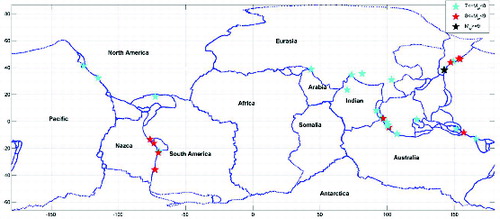
Figure 2. (a) Slip distribution of 2008 Kashmir earthquake (M_w 7.6). (b) Slip distribution of 2010 El Mayor-Cucapah, Mexico earthquake (M_w 7.2). (c) Slip distribution of 2010 Indonesia earthquake (M_w 7.82). (d) Slip distribution of 2010 Maule, Chile earthquake (M_w 8.9).

3. Scaling laws for source dimensions

The first step in characterizing the slip models is to understand the relationship between magnitude or seismic moment and the rupture dimensions. These relations are fundamental to develop source models for simulating ground motions due to large events. In figure 3, the length, width and area of the fault plane as reported in the source inversion are shown as a function of seismic moment. The mean value of the slip is estimated from its spatial distribution on the rupture plane and its variation with seismic moment is shown in figure 3. In the same figure, a straight line of the form (1)

Figure 3. Source dimensions and mean slip as a function of seismic moment: (a) area of the rupture plane versus moment; (b) rupture length versus moment; (c) rupture width versus moment; (d) mean slip versus moment.

where Y is the source dimension, is also fitted to the data. The regression constants for L, W, D and fault area are reported in table 4 along with the standard error. It can be observed that the slope C ₁ for all the four parameters lies in between 0.28 and 0.55, respectively. The theoretical relation between seismic moment (M₀) and the source dimensions is given by (Aki & Richards 1980) (2)

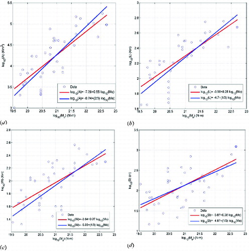
Table 3. Effective source parameters.

					σ (D)
S. no.	(Km)	(Km)	1.0E+04 * sq.km	1.0E+03*(cm)	(cm)
1	184.5	95.9	1.7706	0.4491	243.10
2	192.4	121.4	2.3368	0.2934	96.24
3	132.1	89.3	1.1794	0.1206	58.34
4	99.9	74.6	0.7452	0.0679	30.42
5	43.6	36.7	0.1605	0.7798	347.90
6	175.0	166.6	2.9151	0.1297	186.86
7	302.8	190.2	5.761	0.1531	273.07
8	263.3	175.8	4.6315	0.6073	200.46
9	79.6	22.2	0.177	0.0405	77.72
10	52.3	23.2	0.1215	0.0661	106.79
11	56.9	36.1	0.2056	0.0622	27.07
12	60.4	28.6	0.1729	0.6137	254.38
13	96.6	34.8	0.3364	0.1157	181.95
14	221.5	154.9	3.4333	0.0649	78.77
15	281.2	123.6	3.4772	0.2997	103.61
16	182.6	33.3	0.6095	0.8065	455.48
17	173.4	27.1	0.4712	0.1395	339.42
18	241.8	76.1	1.8412	0.1099	97.42
19	100.1	101.1	1.0124	0.3732	136.66
20	125.7	96.2	1.2096	0.0001	79.70
21	220.3	157.7	3.4759	0.0003	134.75
22	353.0	146.5	5.1724	0.2191	92.36
23	193.4	105.4	2.0386	0.0142	54.57
24	230.9	137.9	3.184	0.1063	39.41
25	153.9	84.5	1.3019	0.1912	75.16
26	84.4	77.1	0.6507	0.0001	23.65
27	115.2	27.6	0.3182	0.0188	36.40
28	191.7	24.3	0.4668	0.2003	361.89
29	243.6	30.6	0.7461	0.4845	250.51
30	90.3	32.4	0.2933	0.0675	58.52
31	39.7	32.0	0.1274	0.4502	153.47
32	37.3	34.3	0.1281	0.4564	154.06
33	77.3	43.3	0.3355	0.2337	90.63
34	37.5	17.4	0.0655	0.2378	114.97
35	178.5	178.6	3.1885	0.6108	321.43
36	483.6	170.2	8.236	0.2057	154.92
37	118.6	13.4	0.1596	0.0576	121.92
38	213.3	68.1	1.4518	0.0711	70.11
39	118.6	83.6	0.481	0.1587	48.62
40	282.4	162.5	4.5908	3.2795	1347.45
41	282.4	162.5	4.5908	3.2795	1347.45
42	282.4	162.5	4.5908	3.2795	1347.45
43	287.6	144.4	4.1549	1.8181	1526.18
44	484.7	194.3	9.4194	1.8136	764.28
45	29.2	36.2	0.1059	0.2992	93.10

Table 4. Scaling relations of slip models log₁₀(Y) = C₀ + C₁ log₁₀(M₀).

Y	C0	C1	σ(ϵ)
L	−3.58	0.28	0.19
W	−3.64	0.27	0.23
A	−7.39	0.55	0.34
D	−5.87	0.38	0.36
σD	−5.49	0.36	0.31
Leff	−3.52	0.27	0.19
Weff	−4.34	0.29	0.21
Aeff	−8.02	0.57	0.31
Deff	−6.50	0.40	0.45
ALA	−8.33	0.56	0.31
AVLA	−6.75	0.47	0.27
ACA	−7.45	0.53	0.29
RDmax	−4.7	0.31	0.35
RLA	−1.39	0.11	0.37
RVLA	−3.97	0.24	0.41

where L and W are the length and width of the fault and D is the average slip. μ is the rigidity of the medium surrounding the fault. If stress drop remains constant, increase in the seismic moment occurs due to proportionately equal changes in L , W and average slip D . The self-similar scaling can be expressed as M₀ ∝ L ^1/3, M₀ ∝ W ^1/3, M₀ ∝ (LW )^2/3 and M₀ ∝ D ^1/3. Assuming the slope from the self-similar scaling, the intercept can be found from the data. The obtained empirical equation assuming self-similarity is shown in figure 3 along with the data. The self-similar scaling equations are reported in table 5 along with the standard error. The obtained slope from the data (C₁) for all the quantities is of the same order indicating self-similar scaling. It can be observed that the source dimensions linearly increases with increasing seismic moment for large events.

Table 5. Scaling relations of slip models assuming self-similarity log₁₀(Y) = C₀ + C₁ log₁₀(M₀); C₁ is fixed.

Y	C0	C1	σ(ϵ)
L	−4.70	0.33	0.19
W	−5.03	0.33	0.24
A	−9.74	0.67	0.36
D	−4.87	0.33	0.37
σD	−4.84	0.33	0.31
Leff	−4.85	0.33	0.20
Weff	−5.16	0.33	0.21
Aeff	−10.02	0.67	0.32
Deff	−5.16	0.33	0.45
ALA	−10.54	0.67	0.33
AVLA	−10.88	0.67	0.33
ACA	−10.36	0.67	0.31
RDmax	−5.47	0.33	0.35
RLA	−6.02	0.33	0.42
RVLA	−5.84	0.33	0.42

3.1. Effective source dimensions

In earthquake source inversion, fault dimensions are generally chosen large to map the entire rupture. It can be observed from figure 2 that slip along the edges of the rupture plane is zero or very small compared to the mean slip. In such cases, the length and the width of the reported slip models will overestimate the true rupture dimensions. Estimating the exact source dimension from the slip distribution is difficult. To circumvent this problem, there have been techniques developed based on empirical approaches. Somerville et al. (1999) defined the rupture dimensions based on the slip distribution. If the slip distribution along the edges of the fault is 0.3 times less than the average slip, the entire row or the column is removed from the rupture distribution. Mai and Beroza (2000) defined the effective source dimensions based on autocorrelation function. To estimate the effective length and width, marginal slip distributions are derived by summing the slip in both the along-strike and down-dip directions. 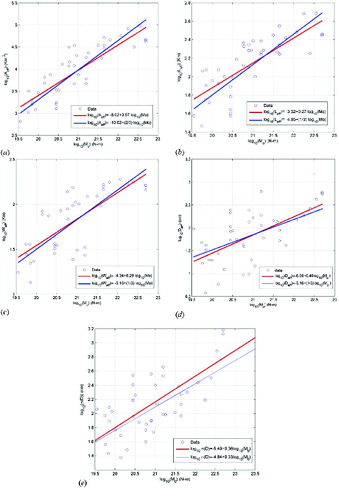The autocorrelation function is estimated and the width of this function is computed as (Bracewell 1986) (3) where W_a is the autocorrelation width and * is the convolution operator. The effective length and width of the rupture plane are estimated from the marginal slip distribution in along- strike and down-dip directions. In a similar fashion, effective length and width have been estimated for all the slip models. These are reported in table 3 for all the 45 slip models. In figure 4, a comparison between the effective area and the area of fault dimensions used in the earthquake source inversion is shown. The ratio between effective dimensions to original dimensions has been estimated. The ratio between effective length to original length lies in between 0.51 and 0.95 with a median value of 0.74. In down-dip direction, the median change in width is 0.76 and it lies in between 0.43 and 0.96 for all the 45 rupture models used in this analysis. The effective area of all the events lies in between 24% and 88% of the original source dimensions. Empirical equations to predict effective source dimensions from seismic moment are derived from the data. The coefficients are reported in table 4. The fitted equations are shown along with the data in figure 5. The self-similar scaling relations by constraining the slope are also shown in figure 5. The effective source dimensions increase with increase in the seismic moment. Since the effective area is less than the original source dimensions, the slip on the fault plane has to be increased to conserve the seismic moment. The average effective slip variation with moment is shown in figure 5(d). The standard deviation around the mean value also increases with increase in the seismic moment.

Figure 4. Comparison between effective and original rupture area.

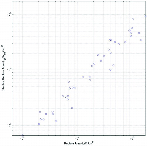
Figure 5. Effective source dimensions and effective mean slip as a function of seismic moment: (a) area of the rupture plane versus moment; (b) rupture length versus moment; (c) rupture width versus moment; (d) mean slip versus moment; (e) standard deviation of slip versus moment.

4. Asperities on the rupture plane

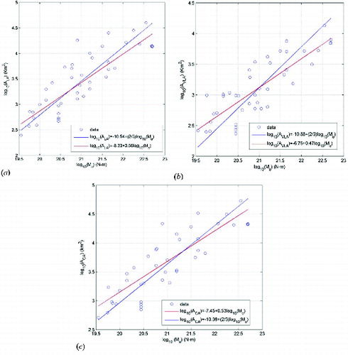
After deriving the equations for estimating the source dimensions, the next step is to understand the regions of concentration of large slip relative to the mean slip on the rupture plane. These regions are known as asperities. There is no guideline available to determine the threshold value of slip to define an asperity. The approaches in the literature have been empirical and based on personal judgement. Somerville et al. (1999) define asperities as rectangular regions whose average slip is 1.5 times more than the mean slip on the entire rupture plane. In this study, the approach of Mai et al. (2005) based on the ratio of slip distribution on the rupture plane to the maximum slip is used to define asperities. The subfaults on which the ratio lies in between 0.33 ≤ D/D_max ≤ 0.66 are taken as large asperity. The regions where the ratio (D/D_max) is greater than 0.66 is defined as a very large asperity. A very large asperity is always enclosed by large asperity. In figure 6, the area of very large asperity (A_VLA) and large asperity (A_LA) are shown as function of seismic moment for all the 45 events. The combined area of asperities (A_CA) is also shown in figure 6(c). It can be observed that asperities increase with increasing seismic moment. Empirical equations between log(A) and log(M₀) are fitted to the data and the constants are found by regression analysis. These are reported in table 4 along with the standard error in the regression. The large asperities occupy about 10%–55% of the effective rupture area, whereas the area of very large asperities is about 2%–40% of A_eff for all the 45 events. The combined area of asperities lies in between 12% and 78% of the effective area. It will be of interest to know how self-similar scaling relations model the data. The self-similar scaling relations are derived by constraining the slope to be 2/3 and the intercept is obtained from the regression on the data. It can be observed that the area of very large asperities deviates from self-similarity, whereas large asperities are closer to the self-similar relations.

Figure 6. Scaling of the size of asperities with seismic moment.

4.1. Location of hypocentre and asperities

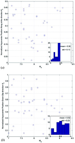
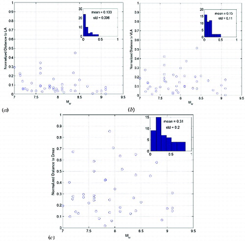
Another important aspect which affects the near-field ground motion is the location of hypocentre and asperities on the fault plane. This information is important to understand the crack propagation during the rupture which can be further used to develop dynamic rupture models. The distance of the hypocentre from the edges of the fault in along-strike (H_x ) and down-dip (H_z ) directions normalized by length and width of the fault is computed for all the 45 slip models. Due to symmetry, the normalized distance in along-strike direction (H_x ) lies in between 0 and 0.5, whereas H_z lies in between 0 and 1. H_x = 0 indicates that hypocentre is located on the edge of the fault, whereas H_x = 0.5 indicates the centre of the fault. Similarly, H_z = 0 denotes the hypocentral location at the top edge of the fault and H_z = 1 denotes the bottom edge of the rupture plane. These non-dimensional quantities are shown in figure 7 as a function of magnitude. It can be observed that H_x and H_z do not show any pattern with M_w. The histograms are also shown in figure 7. The H_x is distributed with a mean of 0.30 and a standard deviation 0.13, whereas for H_z, these two moments are 0.52 and 0.23, respectively. The hypocentre is approximately located at the centre of the fault in down-dip direction.

Figure 7. Normalized hypocentre position in (a) along-strike and (b) down-dip directions.

To understand the relationship between the hypocentre and the location of the asperity, the closest distance to the asperity from the hypocentre is determined from the data. In figure 8, the variation of the closest distance to large and very large asperities from hypocentre is shown as a function of seismic moment. The histograms of these distances are also shown in the same figure. The closest distance increases with increase in the seismic moment. Large asperities are located close to the hypocentre, whereas very large asperities are located at approximately 24 km from the hypocentre. The regions of maximum slip are located approximately at a distance of 50 km from the hypocentre. Empirical equations between distance and moment are derived from the data with and without constraining the slope, and constants are reported in tables 4 and 5. Figure 9 shows the closest distance to asperities normalized by maximum distance to the farthest subfault on the plane, R_max as a function of moment magnitude. It can be observed that they do not show any pattern with M_w. The histograms are also shown in the same figure. It is interesting to note that asperities are not located randomly on the rupture plane but they lie close to the hypocentre.

Figure 8. Scaling of the closest distance to asperities with seismic moment: (a) large asperity; (b) very large asperity; (c) location of maximum slip.

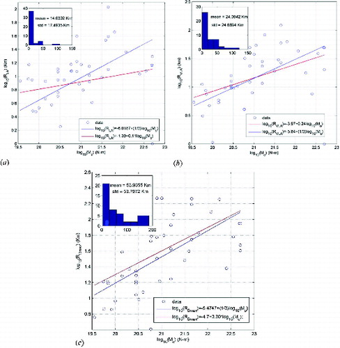
Figure 9. Closest distances to asperities and normalized by maximum distance to the farthest subfault on the plane.

5. Power spectral density (PSD)

The above empirical equations can be used to fix up the rupture dimensions, average slip and location of hypocentre for a given seismic moment. However, to simulate ground motion by source mechanism model requires complete slip distribution on the rupture plane. One requires representation of the slip field in terms of mathematical functions. The previously derived equations provide information on the average properties of the slip field. The possibility of representing the slip field in terms of simple mathematical expressions is ruled out due to the randomness in the derived rupture models. It can be observed from figure 2 that the obtained slip component of large events are erratic which can be attributed to randomness observed in ground motion records. More number of parameters are required to characterize completely the spatial distribution of slip. The only way to model the slip distribution is through stochastic approaches where a few parameters are sufficient to explain the complex data. The two striking features of the slip models are randomness and non-stationarity in their spatial distribution. Assuming the slip as a homogeneous random field, the spatial mean and standard deviation are computed for all the 45 slip models. For estimating the further statistics, the slip field is standardized as (4)

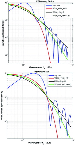
In second-order analysis, the variation of random field models at two different locations is characterized either in space by an autocorrelation function or in the wave-number domain by a PSD. Assuming the slip field as ergodic, two-dimensional PSD (S (κ_x,κ_z)) is obtained from the slip distribution as (5) where κ_x and κ_z are the spatial wave numbers. The obtained standardized slip field is transformed into the two-dimensional wave-number domain using zero-padded grids of size 1024 × 1024 km. The Nyquist wave number in both the directions depends on the size of the subfaults determined from the earthquake source inversion. It can be observed from table 2 that the size of the subfaults is not uniform along the length and width of the fault for all the 45 models. Hence the highest wave number for which the slip model is valid will be different for all the events. The two-dimensional PSD function computed from ‘equation (5)’ for Kashmir earthquake slip model shown in figure 2(a) is shown in figure 10. A random field is known as isotropic, if the correlation is independent of direction (Vanmarcke 1983). It can observed from figure 10 that the correlation structure is different in along-strike and dip-directions indicating that the moment field is anisotropic. In figure 11, the PSD functions at cross sections κ_x = 0 and κ_z = 0 are also shown. There are several theoretical two-dimensional correlation functions available in the literature. Three correlation functions widely used in literature are Gaussian, exponential and von Karman (Mai & Beroza 2002). The expressions for the autocorrelation and PSD for these three random field models are as follows:

Figure 10. Two-dimensional power spectral density function for the slip model of Kashmir event shown in figure 2(a).

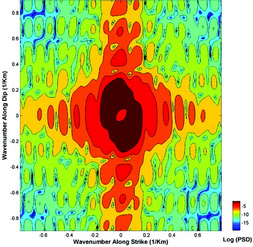
Figure 11. Comparison with the Gaussian, exponential and von Karman PSD at the cross sections κ_x = 0 and κ_z = 0 for the slip model of Kashmir event shown in figure 2(a).

Gaussian: (6)

Exponential: (7)

von Karman: (8) where (9) a_x and a_z are the correlation lengths along x and z-directions, respectively. H is the Hurst exponent and K_H is the modified Bessel function of the first kind. It can be observed that when H = 0.5 von Karman is identical to the exponential PSD. The parameters a_x and a_z of the three random fields are estimated from the slip field by minimizing the mean square error between the computed PSD and the expressions shown in equations (6)–(8). The fitted Gaussian, exponential and von Karman PSD at cross sections κ_x = 0 and κ_z = 0 are plotted in figure 11 along with the data for Kashmir earthquake. Besides, the estimated parameters are also shown in the same figure. The misfit associated with von Karman function is slightly lower than that obtained from exponential and Gaussian function, and hence the slip fluctuation can be modelled as a von Karman random field. Similarly, the correlation lengths are estimated for all the slip models. These are reported in table 6 for Gaussian, exponential and von Karman PSD. The correlation length a_x is much larger than a_z which can be attributed to large length compared to the width of the fault.

Table 6. Estimates of correlation lengths and Hurst exponents, H, for slip models listed in table 1.

	Gaussian		Exponential		von Karman
S. no.	ax	az	ax	az	ax	az	H
1	42	28	23	16	6	4	12.3
2	70	43	43	26	49	31	0.3
3	40	27	22	15	6	4	11.1
4	30	40	16	25	7	10	4.1
5	11	19	6	12	6	12	0.5
6	54	93	30	55	21	37	1.4
7	104	55	60	30	38	20	1.6
8	148	55	73	32	90	41	0.2
9	33	8	20	4	9	2	3.5
10	21	10	12	5	4	2	6.1
11	22	14	12	8	3	2	12.7
12	16	10	9	6	6	2	1.8
13	44	12	27	6	11	3	3.8
14	41	45	22	25	13	14	2.2
15	76	54	43	30	60	43	0.1
16	44	12	27	8	38	11	0.1
17	140	10	76	6	82	6	0.4
18	47	58	28	31	39	43	0.1
19	33	33	18	18	12	12	1.6
20	33	37	20	21	29	28	0.1
21	90	45	48	25	44	22	0.7
22	99	100	56	64	45	50	0.9
23	34	78	20	38	28	50	0.1
24	67	42	35	24	30	21	0.8
25	123	27	69	15	51	11	1.2
26	28	32	15	18	5	6	7.1
27	53	10	33	5	27	4	0.9
28	25	12	14	7	20	10	0.1
29	86	9	44	5	37	4	0.9
30	42	14	26	8	20	6	1
31	15	11	8	6	3	2	6.8
32	12	10	7	5	2	2	7.1
33	42	13	25	8	35	11	0.1
34	16	6	10	3	5	3	2.4
35	39	100	21	79	14	50	1.5
36	63	90	37	50	40	50	0.4
37	115	4	32	3	51	3	0.1
38	117	24	68	13	55	33	0.5
39	17	30	9	18	4	7	4.3
40	81	83	45	50	11	11	13.7
41	81	83	45	50	11	11	13.7
42	81	83	45	50	11	11	13.7
43	92	62	51	36	12	8	14.6
44	150	85	114	48	44	19	4.3
45	8	17	4	10	2	4	4.1

6. Scaling laws for correlation lengths

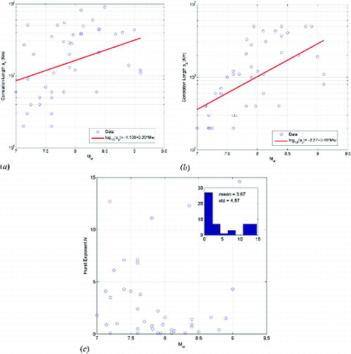
After estimating the spectral parameters from PSD, it remains to identify the patterns with the previous determined effective source dimensions and moment magnitude. Figures 12 and 13 show the variation of correlation lengths of the Von Karman PSD with the M_w, effective length and width of the rupture plane. The correlation lengths increase with increasing source dimensions. The Hurst exponent does not show any pattern with the source dimensions. The variation of a_x and a_z with the source dimensions can be expressed as (10) where Y is correlation length in along-strike and down-dip directions, and X is the M_w, L_eff and W_eff. The coefficients are obtained by regression analysis of the data. These are reported in table 7 along with the standard error. The scaling laws derived from the present study are shown in figures 12 and 13 along with the data.

Table 7. Coefficients for the scaling of correlation lengths a_x and a_z for the autocorrelation function with source parameters log₁₀(Y) = C₀ + C₁ (X).

X	C0	C1	σ(ϵ)
Along-strike (Y = ax)
Mw	−1.1090	0.2903	0.4194
Leff	0.7699	0.0025	0.3649
Weff	0.9705	0.0026	0.4284
Down-dip (Y = az)
Mw	−2.5736	0.4475	0.3700
Leff	0.5171	0.0027	0.3500
Weff	0.4945	0.0056	0.3226

Figure 12. Scaling of correlation length with effective rupture dimensions.

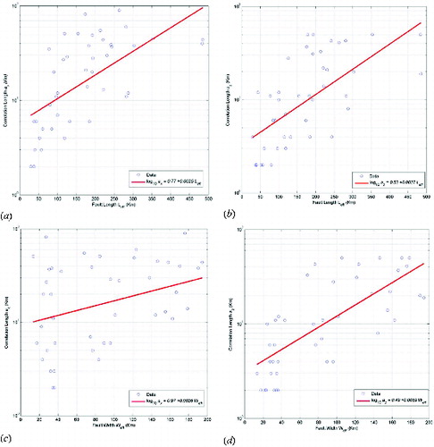
Figure 13. Correlation lengths and Hurst exponent of the von Karman PSD as a function of moment magnitude, M_w.

7. Simulation of the slip field of large events

The proposed methodology for simulating spatial distribution of the slip field is as follows:

1. Fix the initial fault parameters such as strike, dip and rake angle based on the tectonic set-up of the region. Select the moment magnitude, M_w, of the potential earthquake from the past seismicity of the region.

2. Estimate the seismic moment from M_w from the relation of Hanks and Kanamori (1979): (11)

3. Determine the length, width, mean slip, correlation length and standard deviation of slip from source scaling relations using the coefficients reported in table 4. For varying magnitudes, these parameters have been estimated from the scaling relations developed in the present study and is reported in table 8.

   Table 8. Estimates of length, width, correlation lengths(a_x, a_z) and Hurst exponents, H, for slip models for varying magnitudes.

   	Mw
   Slip parameters	7.5	8	8.5	9
   Subfault size, dx (km)	1	1	1	1
   Subfault size, dz (km)	1	1	1	1
   L (km)	100	176	312	551
   W (km)	47	83	146	258
   A (1E+005 sq. km)	0.047	0.146	0.456	1.422
   D (cm)	67	119	211	373
   σD (cm)	72	128	226	399
   Leff (km)	71	125	221	390
   Weff (km)	35	61	108	191
   Deff (cm)	35	61	108	191
   ALA (1E+005 sq. km)	0.012	0.037	0.116	0.370
   AVLA (1E+005 sq. km)	0.005	0.017	0.053	0.169
   ACA (1E+005 sq. km)	0.017	0.055	0.176	0.560
   RDmax (km)	16.94	29.96	52.97	93.65
   RLA (km)	4.77	8.44	14.93	26.39
   RVLA (km)	7.23	12.78	22.59	39.95
   Correlation length, ax (km)	11.70	16.35	22.83	31.89
   Correlation length, az (km)	6.06	10.15	16.99	28.44
   Hurst exponent, H	1.19	1.33	1.49	1.67

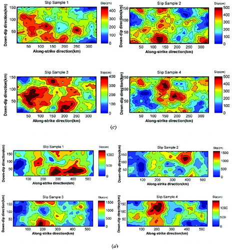
4. Once the correlation lengths are fixed, simulate the standardized slip as a von Karman random field from the spectral representation method of Shinozuka and Deodatis (1996) or Fourier integral method of Pardo-Igu´zquiza and Chica-Olmo (1993). Generate the slip field from equation (4). An ensemble of slip models can be simulated from this procedure. Figure 14(a)–(d) shows the simulated slip samples for M_w = 7.5, 8, 8.5, 9, respectively.

5. The location of the hypocentre can be decided based on the asperity location as shown in figure 8.

Figure 14. (a) Simulated slip samples for M_w = 7.5. (b) Simulated slip samples for M_w = 8. (c) Simulated slip samples for M_w = 8.5. (d) Simulated slip samples for M_w = 9.

8. Summary and conclusions

In this paper, a stochastic kinematic model has been developed to represent earthquake sources for large events. A total of 45 slip models coming from 33 events have been used to develop the model. The development has been done in two stages. In the first stage, scaling relations between seismic moment and source dimensions have been derived from the data. The effective dimensions of the rupture plane are estimated from the autocorrelation width. To conserve the seismic moment, slip on the fault plane is increased by the ratio between area and effective area and effective mean slip is obtained from the data. Scaling laws to estimate source dimensions from seismic moment have been derived from the data. The data also have been used to test self-similarity of earthquakes. Empirical equations by constraining the slope in the regression assuming self-similarity have been derived from the data. It can be observed from figures 3 and 4 that the source dimensions follow self-similarity.

The area of asperities and their location on the rupture plane also have been examined for all the slip models. The asperities have been classified into large and very large asperity based on the ratio of local slip to the average slip on the rupture plane. It is observed that large asperities constitute 10%–55% of the effective rupture area, and very large asperities constitute about 2%–40% of the A_eff, respectively. The area of asperities also increases with increase in the seismic moment. Empirical equations have been developed to estimate the area of asperities from the seismic moment. The large asperities are consistent with self-similarity, whereas the size of very large asperities deviates from self-similarity.

The hypocentre location on the rupture plane does not show any pattern with magnitude, whereas the location of asperities from hypocentre increases with increase in the seismic moment. The closest distance to regions of maximum slip and very large asperity is consistent with self-similarity. The normalized distance from hypocentre to asperities indicates that hypocentres are located closer to asperities.

Modelling the slip distribution on the rupture plane as a random field also has been explored in this paper. This helps to understand the interaction between the slip on the neighbouring subfaults. The two-dimensional PSD is estimated from the slip model by Fourier transform. The correlation lengths are different in along-strike and down-dip directions indicating that the slip field is anisotropic. Gaussian, exponential and von Karman PSD are fitted to the data by estimating the correlation lengths along the length and width of the rupture plane. It is observed that von Karman PSD models the spectral decay of the slip field better than Gaussian and exponential models. The correlation lengths increase with increase in the magnitude of the event. Empirical equations to estimate the parameters in the von Karman PSD from magnitude are derived from the data.

The results presented in this paper will be of use to engineers in simulating ground motion for large events. Given a particular fault and magnitude, the developed model can handle uncertainties in the slip distribution. The seismic moment can be estimated from the magnitude through empirical relations. The length, width and mean slip can be estimated from equations (1) and (2) from the seismic moment. Once the rupture dimensions are known, correlation lengths can be determined by using equation (10) and coefficients reported in table 7 from the magnitude of the event. Sample realizations of the standardized slip field can be simulated by the spectral representation of Shinozuka and Deodatis (1996) by replacing sequences of random phase angles. The hypocentre should be located closely to the location of large asperity on the rupture plane. An ensemble of slip fields can be generated from this procedure. There are several methods available in the literature to generate ground motion time histories for a given slip model (Douglas & Aochi 2008; Raghukanth 2008). Several samples of ground motion time histories can be generated from this procedure. The developed stochastic source model for large events will find applications in simulating ground motion for scenario earthquakes in seismic hazard analysis. The equations developed in this study have to be updated as more slip models become available.

References

- Aki K, Richards PG. 1980. Quantitative seismology: theory and methods. Vol. 1. New York (NY): WH Freeman; p. 1–700.
- Bird P. 2003. An updated digital model of plate boundaries. Geochem Geophys Geosyst. 4:1525–2027.
- Bracewell RN. 1986. The Fourier transform and its applications. New York (NY): McGraw-Hill.
- Douglas J, Aochi H. 2008. A survey of techniques for predicting earthquake ground motions for engineering purposes. Surv Geophys. 29:187–220.
- Hanks TC, Kanamori H. 1979. A moment magnitude scale. J Geophys Res. 84(B5):2348–2350.
- Hartzell S, Harmsen S, Frankel A, Larsen S. 1999. Calculation of broadband time histories of ground motion: comparison of methods and validation using strong ground motion from the 1994 Northridge earthquake. Bull Seismol Soc Am. 89:1484–1506.
- Hartzell S, Heaton T. 1983. Inversion of strong ground motion and teleseismic waveform data for the fault rupture history of the 1979 Imperial Valley, California, earthquake. Bull Seismol Soc Am. 73:1553–1583.
- Hartzell S, Liu P. 1995. Determination of earthquake source parameters using a hybrid global search algorithm. Bull Seismol Soc Am. 85:516–524.
- Ji C, Wald DJ, Helmberger DV. 2002. Source description of the 1999 Hector mine, California, earthquake, Part I: wavelet domain inversion theory and resolution analysis. Bull Seismol Soc Am. 92(4):1192–1207.
- Lavallée D, Liu P, Archuleta RJ. 2006. Stochastic model of heterogeneity in earthquake spatial distributions. Geophys J Int. 165:622–640.
- Mai PM, Beroza GC. 2000. Source scaling properties from finite-fault-rupture models. Bull Seismol Soc Am. 90(3):604–615.
- Mai PM, Beroza GC. 2002. A spatial random field model to characterize complexity in earthquake slip. J Geophys Res. 107:1–28.
- Mai PM, Spudich P, Boatwright J. 2005. Hypocenter locations in finite-source rupture models. Bull Seismol Soc Am. 95:965–980.
- Pardo-Igu´zquiza E, Chica-Olmo M. 1993. The Fourier integral method: an efficient spectral method for simulation of random fields. Math Geol. 25:177–217.
- Raghukanth STG. 2008. Modeling and synthesis of strong ground motion. J Earth Syst Sci. 117:683–705.
- Raghukanth STG. 2010. Intrinsic mode functions of earthquake slip distribution. Adv Adapt Data Anal. 2(2):193–215
- Raghukanth STG. 2011. Seismicity parameters for important urban agglomerations in India. Bull Earthquake Eng. 9(5):1361–1386.
- Raghukanth STG, Iyengar RN. 2008. Strong motion compatible source geometry. J Geophys Res-Sol Ea. 113(B4):B04309. doi:10.1029/2006JB004278
- Raghukanth STG, Iyengar RN. 2009. Engineering source model for strong ground motion. Soil Dyn Earthq Eng. 29:483–503.
- Shinozuka M, Deodatis G. 1996. Simulation of multi-dimensional Gaussian stochastic fields by spectral representation. Appl Mech Rev. 49(1):29–53.
- Somerville P, Irikura K, Graves R, Sawada S, Wald D, Abrahamson N, Iwasaki Y, Kagawa T, Smith N, Kowada A. 1999. Characterizing crustal earthquake slip models for the prediction of strong ground motion. Seismol Res Lett. 70(1):59–80.
- Vanmarcke EH. 1983. Random fields: analysis and synthesis. Cambridge (MA): MIT Press.