Elementary analysis on the bed-sediment entrainment by debris flow and its application using the TopFlowDF model

Abstract

The Geographic Information System (GIS)-based TopFlowDF model is an effective simulation tool to analyse the debris-flow propagation on the fan. It has been validated in the previous research works and shows a satisfactory accuracy. We review the framework of the model in this paper and discuss that the simulation results are rather sensitive to the input conditions (e.g. the user-defined start point and debris-flow volume). In fact, previous studies have elucidated that sediment entrainment by debris flow conspicuously influences these input conditions. In this paper, we develop an elementary static approach with a three-layer model to estimate the entrainment and determine the amplification of total mass volume and peak discharge. Subsequently a new concept of “critical line” is proposed to detect the erodible reaches in the channel. Two cases in Japan and Norway are selected to illustrate the approach; analytical results show a good agreement with the in situ survey. The presented approach can provide a better solution to the input conditions as required by TopFlowDF model.

1. Introduction

Debris flows pose immense impact to human lives and infrastructure facilities in mountainous regions around the world. For instance, Japan recorded totally 1,558 debris-flow events between the years 2007 and 2012, which caused death of 162 human beings and damages to 394 buildings (Han et al. 2012). To describe the propagation and run-out characteristics, numerical simulation models are proposed (e.g. Hungr & McDougall 2005; Chen et al. 2006; Mangeney et al. 2007; Pirulli & Pastor 2012). These methods use the finite volume method or the finite difference method to solve the depth-average form of the shallow water equations over complex three-dimensional (3D) topographies. Different rheological models are incorporated, such as the dispersive model (Bagnold 1966), dilatant model (Takahashi 1978; Hungr et al. 1984), Voellmy model (Christen et al. 2010) and viscous-plastic-collision model (O’Brien et al. 1993; O’Brien 2006). However, on the one hand, solving shallow water equations is time-consuming. On the other hand it is difficult to estimate the rheological parameters in these methods, which may somewhat influence the simulation results (Duzgun et al. 2002; Ocakuglu et al. 2002; Takahashi 2007).

Up-to-date research works use the probabilistic approaches to predict debris-flow run-out on the fan (O’Callaghan & Mark 1984; Quinn et al. 1991; Tarboton 1997; Gamma 2000; Hürlimann et al. 2008; Prochaska et al. 2008; Horton et al. 2013). Remarkable work done by Scheidl and Rickenmann (2011), the model, named TopFlowDF, incorporated a Monte Carlo method based routine algorithm into a constant discharge model (Takahashi 1991), and showed a high executive efficiency and satisfied accuracy (Huber 2012). This model requires input parameters consisting of (1) total mass volume, (2) a mobility coefficient, (3) a starting point (SP) of the deposition, and (4) a digital elevation model (DEM) data of the fan area. It has been revealed that parameters (1)–(4) influence the simulation results, but (1) and (3) show more conspicuous significance. In practice, it requires empirical calibration and trial-and-error adjusting on these input parameters to obtain an appropriate result.

However, it is not easy to determine the total mass volume and SP sometimes. Research works have long revealed that debris flow is generally induced by a small landslide on the steep slope (>25° or 30°), and culminates when surging mixtures of fragmented rock and muddy water disgorge from canyons onto the channel bed (e.g. Glade 2005; Iverson et al. 2011; Chen & Yu 2011). In this process, several lines of evidence suggest an important role of sediment entrainment that debris flow can grow manyfold both in size and magnitude as it descends the steep and debris-mantled slopes (Hungr et al. 1984; Chen et al. 2005; Hungr et al. 2005; He et al. 2007). A worth mentioning event was well recorded by King (1996), total mass volume of the debris-flow event grew 50 times compared to the initial volume. In addition, because erosion tracks are often hidden by subsequent flows, it is hard to distinguish the flow deposit and the underlying erodible layer (Mangeney 2011), as well as the SP position in a gully.

In this study, we review the framework of TopFlowDF model, propose a static equilibrium model to determine the total mass volume and a new concept of “critical line” to identify the SP location of deposition, which will be instrumental to improve the accuracy of the input parameters in TopFlowDF model. The debris-flow cases at Yohutagawa watershed in Japan and Fjaerland area in Norway are used to illustrate this approach, and accuracies are assessed by comparing TopFlowDF simulation with observation.

2. Framework of TopFlowDF model

TopFlowDF model was proposed by Scheidl and Rickenmann (2011). It originated from TopRunDF (Scheidl & Rickenmann 2010) model, which is regarded as a probabilistic approach based on the empirical relationship between total mass volume and inundated area. TopFlowDF model consists of two major parts, the flow algorithm to determine the depositional flow path, and dynamic model to assign the deposition depth on each flow path.

2.1. Flow algorithm

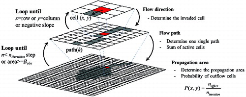
The flow algorithm is important, since it determines the propagation of debris flow. There are many different algorithms that can simulate overland flow in 3D topography (e.g. O’Callaghan & Mark 1984; Quinn et al. 1991; Tarboton 1997; Gamma 2000; Hürlimann et al. 2008; Horton et al. 2013). TopFlowDF model uses the analogous algorithm by Gamma (2000) to determine the flow direction and single flow path, then combines with a Monte Carlo iteration to simulate the propagation region of debris flow. The basic concepts of this model are summarized as three steps below.

First, debris flow is regarded to start in a central cell (user-defined start point) and will invade one of its eight neighbouring cells i, probabilities of these eight possible directions P_i are defined as (1) where θ_i is the slope gradient from the central cell towards cell i. To save the computation time, negative slope (tan θ_i < 0) is treated as 0, and cells with negative slope are regarded as boundary confinement which avoid the eventual backward propagation. The cell where the debris flow will invade is then determined using a random number m (ranging from 0 to 1), generator and the following condition should be satisfied: (2) where S_i and S_i-1 are the accumulated probabilities of cell i and cell i − 1, and defined as (3)

Second, the procedure from equations (1)–(3) is repeated to obtain a single flow path. The single flow path should end when any of the boundary conditions (e.g. negative slope, boundary of the DEM data) are reached.

Third, when boundary conditions of one path are reached, the central cell of the next step is moved back to the SP we firstly defined; in this way, many single flow paths can be obtained by repeating the procedure we demonstrated above. Then all the paths are combined and form a propagation region, the Monte Carlo iteration will end when the simulated planimetric deposition area is larger than the observed or empirically calculated deposition area. The probability of each outflow cell can be computed using the following equation: (4) where x, y denotes the position of the cell, n_affect denotes the number of debris-flow trajectories that invade this cell, n_iteration denotes the number of total Monte Carlo iterations. The total post-entrainment volume will be assigned in proportion to the outflow probability of each flow cell.

Finally, once the propagation region is determined, the total post-entrainment volume, discharge and flow depth will be assigned on each single path according to the probability of each outflow cell. The whole procedure is illustrated in figure 1.

Figure 1. Schematic illustration of the Monte Carlo iteration combined flow algorithm.

2.2. Dynamical model

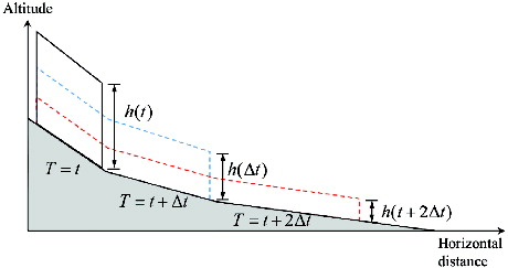
The propagation area simulated by the procedure above consists of many single routines. But for practical purpose, people are also concerned about the deposition depth and velocity distribution on the alluvia fan. Hence, TopFlowDF uses the constant discharge model (Takahashi 1991) to assign the volume to each outflow cell. The constant discharge model can be expressed as (5) where v is the velocity of debris flow, t is the time, U denotes the driving component of debris-flow mass and G denotes the resistance component. (6) (7) where h is the flow height, g is the gravity acceleration, θ, θ′ denote the inclined angle of previous direction and direction of this step, respectively and S_fric denotes the friction coefficient of debris flow, which must be greater than 1.0.

The constant discharge model indicates that the total discharge assigned to the single routine should be constant. It means that the flow depth will get thinner and thinner with time (figure 2). Another confinement is defined that the propagation routine will end when the value of velocity or flow depth is less than 0.001.

Figure 2. Illustration of the constant discharge model of debris flow.

2.3. Sensitivity of the input conditions

TopFlowDF model is a semi-empirical simulation method, the main advantage of this model is that it uses neither time-consuming data (Vasiliou et al. 2011), nor some hard-to-measure rheological parameters. Although the accuracy is satisfactory, simulation results are still rather sensitive to the required input conditions, including (1) DEM data with high-enough resolution, (2) a mobility coefficient, (3) total mass volume, and (4) SP position (a user-defined point where deposition begins). Input conditions influence the deposition scale and pattern prominently, and (3) and (4) show more conspicuous significance (Scheidl & Rickenmann 2011).

Taking Brichboden debris-flow event (Scheidl & Rickenmann 2010) for example. Different values of input parameters are used to illustrate the sensitivity (figure 3). Obviously, simulated propagation of debris flow is rather sensitive the total mass volume and SP position. Figures 3(a) and (b) show the conspicuous different propagation regions applying different SP position, while figures 3(a) and (c) show the different deposition depths applying different mass volume, a larger mass volume will generate a deeper deposit.

Figure 3. Comparison of simulation at Brichboden debris flow with different input parameters: (a) original input parameters of Brichboden case; (b) SP position is moved about 50 m upstream; (c) total mass volume is enlarged from 4,000 to 6,000 m³.

To address this problem, we focus on these two input parameters, and propose a rational approach using a new erosion analysis method and a concept of “critical deposition line”. The study is supposed to provide a better solution to the key parameters of TopFlowDF model.

3. Analytical model for estimating entrainment

3.1. Description of the model

Previous studies indicated that the sediment entrainment occurs when bed shear stress of flow is sufficiently high to overcome basal resistance of the bed and incorporate this part of the bed into the flow (Medina et al. 2008). In this paper, we employ a three-layer model to conduct the static analysis as shown in figure 4. Analogous models described by Iverson (2012), Hungr et al. (2005) and Medina et al. (2008) usually consist of a flow layer with a free top surface, an erodible bed layer with a moveable bottom, and a deeper substrate that cannot be entrained. The model employs Cartesian coordinate system, in which x points to the downstream direction. Variable z denotes entrainment depth along the upward, normal direction to the slope, and y points to the cross-slope direction.

Figure 4. Schematic illustration of the three-layer model: (a) channel cross section; (b) AA′ longitudinal section; (c) plane view; (d) generic element. The variables used in the entrainment model include the following: h is the thickness of the moving mass; z is the entrainment depth; b denotes the channel width; θ_c is the slope angle of the channel; τ_d is the shear stress posing by the debris flow; R₁ is the basal resistance; R₂ is the side resistances; γ_d, γ are the density of the debris-flow mass and bed sediment, respectively; c_v is the volume concentration of the debris flow; c, ϕ are the cohesion and internal friction angle of the sediment, respectively.

To conduct the analysis, the bed sediment is supposed to behave as a rigid-plastic solid and its strength can be described by the Mohr–Coulomb shear strength equation, and the shearing strength along the potential failure can be described by (8) where c is cohesion at potential failure, φ is angle of internal friction at potential failure in degree, τ is the shearing strength and σ is normal stress. Debris-flow fluid behaves as a Newtonian turbulent flow, of which turbulent and viscous stress dominates rather than dispersive stress or particle friction, and the base shear resistance τ_d of this rheological model can be described as follows (Hungr & McDougall 2009): (9a) where γ_d is specific weight of debris-flow fluid, v is depth-averaged velocity, n_c is the Manning's roughness coefficient and h is flow depth of the debris flow. Average velocity of debris-flow mass can be estimated by wide-accepted Manning equation (Chen et al. 2007; Han et al. 2014): (9b) where a is an empirical constant.

3.2. Static equilibrium analysis

Soil mechanics concepts and the infinite slope stability theory (Morgenstern & Sangrey 1978) can be used to describe the static equilibrium of the model. In figures 4(b) and (d), the weight of generic sediment element and debris flow equals (10) where γ is saturated specific weight of bed material (kN/m³), γ_d is specific weight of debris-flow fluid (kN/m³), h is debris-flow depth (m), z is the unknown unstable depth of bed material (m) and b is channel path width at the generic element location (m). Normal total stress and shearing stress at the entrainment base are (11) (12) where θ_c is the channel bed inclined angle in degree. According to Takahashi (1978), pore pressure at the base of generic element equals (13) The shear strength of the base given by Mohr–Coulomb shear strength equation is (14) in which c is the cohesion at potential failure (kPa), φ is internal friction angle in degree.

Additionally, the effects of lateral confinement by both the sidewalls may provide resistant force and stabilize the bed layer. Sidewall resistance can be also calculated by Mohr–Coulomb failure criterion. According to Jaky (1944), the lateral normal stress is transferred from the vertical normal stress, with the ratio of K: (15) where σ_v(z) is the horizontal normal stress at depth z (kPa), σ_h(z) is the vertical normal stress (kPa), for its abbreviated but widely accepted form, K equals the following equation (Wang & Yen 1974): (16) Given an infinitesimally thin layer of bed sediment with dz in height, the vertical normal stress increment dσ_v is (17) The vertical pressure at the base of generic element equals (18) Shear strength of both sides given by Mohr–Coulomb shear strength equation is (19)

For debris-flow fluid, tractive force F_d = τ₁b, basal shear resistance τ_d of the Newtonian turbulent rheological model can be described by equation (9). The main condition for bed entrainment is that bed shear stress of flow F_d is sufficiently high to overcome the total resistance of bed. The static equilibrium between the drag forces of debris flow and resistance forces of sides and bottom reduces to (20) To solve the unknown variable z, equation (20) can be simplified as a positive solution of the quadratic equation: (21a) where (21b) (21c) (21d)

3.3. Amplification of mass volume and peak discharge

Equation (21) computes the entrainment depth at an individual reach i, the increment of debris-flow volume due to entrainment can be expressed by (22) where ΔV(i) is the volume increment, and L(i) is the length of each individual reach. z(i) and b(i) denote the average entrainment depth and path width of each individual reach i, respectively.

Accompanying with the enlarged debris-flow volume, the peak discharge of the debris flow should gradually increase from upper reach to lower reach. It has been widely accepted that the peak discharge increases with the total mass volume. Rickenmann (1999) provides a simple law to describe this. (23) where a₁ and a₂ are the coefficients depending on the type of debris flow and geometry of the temporary reservoir, and a₁ = 0.135, a₂ = 0.78 are determined (Mizuyama et al. 1992); V denotes the debris-flow volume (m³). Equation (23) implies that the peak discharge Q should be in proportion to . We employ this law and propose an elementary model (figure 5) to estimate the amplification of the peak discharge. The increment of the peak discharge is in proportion to the increment of the mass volume. Then equation (23) reduces to (24)

Figure 5. Schematic illustration of the peak discharge amplification.

Figure 6. Illustration for the new concept of critical line. (a) Example of critical line with φ = 28° and c = 8.0 kPa. (b) Example of critical line with φ = 20° and c = 8.0 kPa. (c) Example of critical line with φ = 28° and c = 16.0 kPa. (d) Schematic illustration for the new concept of critical line. To view this figure in colour, please see the online version of the journal.

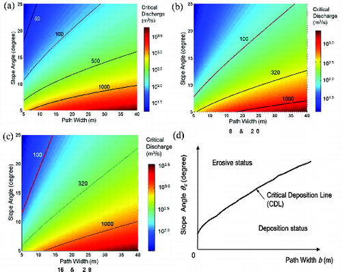
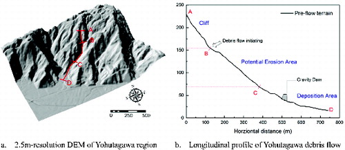
Figure 7. Topography of Yohutagawa debris flow channel.

where Q(i+1) denotes the increased peak discharge which will be used to compute entrainment for the next reach i + 1. In this way, as illustrated in figure 5, the amplification of the peak discharge at each individual reach can be computed.

4. Concept of critical line to detect entrainment reaches

4.1. Critical condition of sediment entrainment

Many in situ surveys (e.g. Bagnold 1966; Takahashi 1991; May & Gresswell 2004; Brayshaw & Hassan 2009) suggested a major role of topography on the entrainment process, i.e. that debris flow often entrains bed sediment when descending a steep and confined slope, and deposits at the wider and flatter alluvial fan of the downstream. Cenderelli and Kite (1998) observed a sudden transition between entrainment and deposition in most of the cases, we infer that critical condition of the sediment exists at the transition places, where the distinct change of slope, or the sudden broadening of channel causes the abrupt decrease of the flow momentum. At the transition place, the entrainment depth of debris flow should satisfy the following condition: (25) The solution of equation (25) applies if the term A₃ in equation (21) equals 0. Then equation (25) reduces to (26a) Explicit solution for equation (26a) is difficult to attain directly. For this reason, equation (26a) is rewritten in a more compact form (26b) Equation (26b) computes the relevant debris-flow depth when sediment is at critical condition. It indicates that the depth of debris flow h should be greater than h_critical in order to provoke the entrainment. A MATLAB code was developed to calculate the approximate solution to equation (26b). However, in practice, h is not easily measured. Hence, we use a more intuitive parameter, the peak discharge Q, to identify the critical condition of bed sediment. Previous research works (Rickenmann 1999; Chen et al. 2007; Han et al. 2014) have validated that Q is the product of the velocity and the area of the cross section where debris flow passes through. It can be computed by (27) The parameters (θ_c, b) are defined as topographic variables. Equation (27) demonstrates that the critical discharge Q_critical depends on the topographic variables. The peak discharge Q of debris flow has to be greater than this critical discharge Q_critical to provoke the bed entrainment.

Three groups of typical parameters (see table 1) are used to illustrate the distribution of the critical discharge. It can be plotted with different micro-geometry variables as shown in figures 6(a)–(c). Colour bars in the figure denote the different values of the critical peak discharge (log₁₀Q_critical).

Table 1. Typical value of parameters used in the illustration of the approach.

	γd (kN/m^3)	γ (kN/m^3)	nc	c (kPa)	φ (degree)	b (m)	θc (degree)
Group a	17.5	26.5	0.15	8	28	5–40	5–25
Group b				8	20
Group c				16	28

Figures 6(a)–(c) show the critical peak discharge versus the channel slope and path width. The figures show that the critical peak discharge will be greater with the increase of the path width and decrease of the channel slope. It can be explained by the fact that entrainment rarely occurs on a wider and flatter topography, unless the discharge of debris flow is large enough to provoke the erosion. Setting the peak discharge of the event 100 m³/s, it can be plotted as a contour line in the figure. For instance, the red line in figure 6(a) denotes the critical discharge which equals the assumed value, if the path width is 20 m, the slope angle should be larger than 20° to provoke the entrainment.

4.2. The concept of critical line

One can see that figure 6 is divided into two parts by the red line; upper one has a narrow and cliffy topography, while lower one has a flatter and gentle topography. It is obvious that in the upper part where real peak discharge is larger than the critical value, bed sediment will be unstable and debris flow will become erosive, this part is recognized as entrainment region. While in lower part, real peak discharge is not large enough to meet the minimum requirement for erosion, debris flow will deposit here and this part is recognized as stable region, as illustrated in figure 6(d). For this reason, the red line is defined as critical line, the concept of which was firstly presented by us in risk assessment of earthquake-triggered landslides (Chen 2008).

The critical line can be further used to detect the entrainment reaches in a channel. Topographic variables (θ_c, b) of the individual reach can be systematically measured from top to bottom in DEM in ArcGIS. The topographic variables (θ_c, b) drop a scatter in the figure of critical line, the status of the sediment can be determined by the region to which the scatter belongs. In this way, entrainment reaches can be detected to decide the precise SP position for TopFlowDF model.

5. Case study

Two debris-flow events are selected to demonstrate this approach. One is Yohutagawa debris flow in Amamioshima, Japan (Wu et al. 2013), and the other is glacial lake outburst triggered debris flow in Fjaerland area, Norway (Breien et al. 2008).

5.1. Description of two debris-flow events

5.1.1. Yohutagawa debris flow (28°24′ N, 129°31′ E)

Triggered by heavy rainfall brought by Typhoon Megi, a debris-flow event occurred on Oct. 20, 2010, at Yohutagawa terrain (Amami Oshima, Japan). Heavy deposits entrained by debris flow damaged two buildings but luckily without any deaths. The watershed is approximately 0.24 km² in area, and 750 m in channel length.

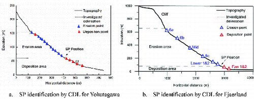
Three evident segments of the slope profile can be divided as shown in figure 7(b). Slope higher than 155 m with 22.57° in average is recognized as initiation area, where potential collapse is 3.4 m in depth and 5,843 m³ in initial volume. Slope with elevation between 155 and 65 m and 18.16° in average is recognized as erosion area, where bed material of channel is supposed to be eroded and transported to downstream, and the channel bed width varies from 12 to 5 m in this area. Slope which is lower than 65 m with 8.94° in average angle is recognized as deposition area, where entrained and transported sediments are supposed to deposit, and channel bed width varies from 15 to 40 m, total inundated area is about 11,644 m². Evident erosion trail was also observed along the path, with erosion depth ranging from 0.5 to 2.0 m, total eroded mass volume might be estimated as 2,854 m³.

Detailed data of this event were investigated by Kokusai Kogyo Co., LTD (KKC), including DEM topography data with a resolution of 2.5 by 2.5 m, aerial images with a resolution of 0.5 by 0.5 m both at pre-hazard and post-hazard.

5.1.2. Debris flow in Fjaerland area

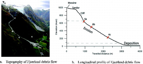
A debris-flow event of Fjaerland occurred on May 8, 2004. It was triggered by the flood due to the failure of a natural moraine ridge dam of glacial lake (figure 8(a)). The average slope gradient of the channel is about 17°, and varies from 25° of entrainment region to 8°–10° of deposition fan (figure 8(b)). The top width of bed surface increases from 26 m upstream to more than 42 m downstream. Although initial volume was rather small (25,000 m³), strong erosion evident was observed along the path, entrainment depth can reach 5.0–8.0 m, causing the total mass volume to increase to 240,000 m³ when rushing to the fan.

Figure 8. Topography of Fjaerland debris flow channel (modified from Breien et al. 2008).

5.2. Detection of entrainment reaches using critical line

Values of relevant variables are listed in table 2. In the 2010 Yohutagawa debris-flow event, precise in situ tests were conducted and results were well documented. Geotechnical tests on the samples revealed that the appropriate extent of internal friction and cohesion should be 30.05 ± 1.55° and 10.0 ± 0.5 kPa, respectively. The samples of the sediment also had volumetric water contents of 0.13 ± 0.05 (saturated density of 23.60 ± 1.10 kN/m³). We use the median of the values of these parameters. The other worth mentioning parameter is peak discharge; it was estimated by the local governments that the peak discharge was around 100 m³/s. We verify this value by equation (23) as summarized by Rickenmann (1999, 2005) that Q is likely to be 117.03 m³/s. However, it was observed at the downstream that velocity is around 2–3 m/s and the active cross-sectional area is 31.86 m² (1.8 m in mud depth and 17.7 m in channel width). It implies that the discharge should be 63.7–95.6 m³/s. In the analysis, considering the theoretical and observed values, we use the mean value 79.7 m³/s to represent the peak discharge.

Table 2. Parameters used in the analysis.

				Fjaerland case
	Parameter		Yohutagawa case	Set 1	Set 2	Set 3
Debris flow property	γd	(kN/m^3)	17.3	15.0
	γw	(kN/m^3)	10.0	10.0
	c0		0.44	0.31
	Q0	(m^3/s)	79.7	750
	V0	(m^3)	5,843	25,000
Bed material property	γ	(kN/m^3)	23.6	24.0
	γs	(kN/m^3)	26.5	26.5
	c	(kPa)	10.0	6.0	12.0	18.0
	φ	(degree)	30.05	30.0	26.0	22.0
	nc		0.25	0.125

While parameters for the Fjaerland debris-flow event are obtained by back-analysis according to the description in Breien et al. (2008). Because Fjaerland debris flow was described to be highly erosive, lower sediment concentration and fluid density should be involved based on the conclusion proposed by Takahashi (2007, 2009), here 15.0 kN/m³ of density and 0.31 of sediment concentration rate advised by Blijenberg (2007) are assumed. Additionally, equation (23) may lead to a too large value (more than 2000 m³/s) in this event; a back-analysis method is adopted to estimate the peak discharge. According to the flow-depth trail in the photo, area of cross sections may be around 120–160 m², and estimated velocity was demonstrated as 3–6 m/s by the author, hence we infer that the peak discharge may be around 700–800 m³/s, here median is utilized.

In Fjaerland debris-flow event, focus is put on the soil strength variables (c, ϕ). Here three sets of rational cohesion c are assumed (table 3), and corresponding friction of bed material can be back-calculated by equations (21a)–(21d), since detailed channel width, slope gradient and observed erosion depth at Lower 1 position are illustrated in the literature.

Table 3. Possible bed material properties verified by erosion depth at Lower 1 position.

	Assumed value
	c (kPa)	φ (degree)	b (m)	θc (degree)	zcalculated (m)	zinvestigated at Lower 1 (m)
Set 1	6.0	30.0	33	15	4.47	4.30
Set 2	12.0	26.0			4.43
Set 3	18.0	22.0			4.22

However, in other locations of Fjaerland gully, discrepancy that entrainment depth increases with the decrease of the slope angle was observed. This can be explained in part by the feedback phenomenon and needs further study.

Values of the debris-flow property and bed material property in both cases are given in table 2, critical line can be determined. Figure 9 shows the critical lines of the 2010 Yohutagawa debris flow and the Fjaerland debris flow, detected entrainment and stable reaches are displayed by different colours, blue colour stands for the entrainment status, while red colour stands for the stable status. Labels around the symbols represent the index of the individual reaches, numbers stand for the mean elevation value of reaches in the Yohutagawa debris flow, while texts stand for the descripted location of points in the Fjaerland debris flow.

Figure 9. Determination of critical line for both the two cases. To view this figure in colour, please see the online version of the journal.

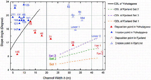
As shown in figure 10, owing to the detailed data in Yohutagawa debris flow, entrainment reaches are well detected by the critical line. The SP position should locate in the 15-m-long reach between 55 and 66 m in elevation. For Fjaerland debris flow, compared to the illustration in the literature, SP position should locate in the reach between Lower 2 and Fan 1, this description fits well with the detection by the critical lines of Set 2 and Set 3. Considering severe erosion along the path, the critical line determined by Set 2 is used, that channel bed mass is considered as silt soil or clay. From figure 10, it can be found that SP position of both the two cases is precisely detected, as compared with investigation or description at post-hazard.

Figure 10. SP position identification by the concept of critical line for both the two cases.

5.3. Simulation of Yohutagawa event using TopFlowDF

Because the detailed DEM data of Fjaerland debris flow are not yet available, only the 2010 Yohutagawa debris-flow case is simulated using TopFlowDF model. Table 4 lists the topographic variables compiled from DEM in ArcGIS 10.1. The detected entrainment region by the critical line is further dispersed into 13 reaches, with about 10–20 m in length, erosion depth of each reach can be calculated by equations (21a)–(21d), total eroded mass volume can be calculated by equation (23), which is about 3,031.81 m³. Total involved mass volume is then calculated by equation (23), as about 8,874.81 m³. Compared to the investigated value 8,697 m³, it is only 2.1% in error.

Table 4. Geometry parameters and calculation results for total mass volume of Yohutagawa debris flow.

i	b(i)	ΔL(i)	θ(i)	v(i)	h(i)	z(i)	ΔV(i)	Q(i)	V(i)
	(m)	(m)	(degree)	(m/s)	(m)	(m)	(m^3)	(m^3/s)	(m^3)
1	10.00	9.49	18.31	2.69	2.96	0.96	92.10	79.70	5,843.00
2	8.00	21.36	15.22	3.30	3.15	0.48	82.02	80.68	5,934.10
3	7.00	19.02	7.52	2.82	4.26	0.00	0.00	81.46	6,016.12
4	12.00	11.89	17.26	2.91	2.35	0.55	78.31	81.46	6,016.12
5	8.00	25.99	19.75	3.63	2.94	1.47	305.92	82.31	6,094.43
6	10.00	14.14	23.75	3.68	2.58	3.06	432.44	85.65	6,400.35
7	8.00	14.47	17.26	3.74	3.43	0.97	112.74	90.56	6,832.79
8	5.00	26.08	19.79	4.58	4.16	1.45	189.17	91.92	6,945.53
9	8.00	23.80	19.18	3.81	3.23	1.49	283.88	94.23	7,134.70
10	6.00	31.62	22.68	4.61	3.75	2.26	428.36	97.78	7,418.57
11	9.00	28.78	18.30	3.75	3.28	1.37	354.02	103.33	7,846.93
12	9.00	20.99	18.72	3.80	3.29	1.54	290.75	108.18	8,200.95
13	10.00	21.13	19.39	3.69	3.05	1.81	383.11	112.36	8,491.70
Final							3,031.81	112.36	8,874.81

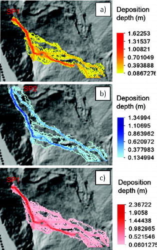
To start simulation, mobility coefficient k should be first calculated in order to continue the back-analysis; mobility coefficient can be computed as(28) where k_Bback is dimensionless mobility coefficient for back analysis. B_obs is the investigated perimeter area of deposits (m²), which can be directly measured by post-hazard images or field investigation. The observed inundated perimeter B_obs and total calculated mass volume V are given prior, k_Bback is estimated as 26.5, and Monte Carlo Iteration (MCI) number is advised as 50 according to Scheidl and Rickenmann (2010). Simulation results obtained by TopFlowDF are shown in figure 11(a). Observed deposition area and simulated deposition area are 12,113 m³ and 11,644 m³, respectively, with average deposition depth of 0.72 m.

Figure 11. Comparison of debris-flow affected area: (a) hazard simulation by improved TopFlowDF approach with k_Bback = 26.5; (b) hazard prediction by improved TopFlowDF approach with k_Bpred = 119; (c) field investigation conducted by KKC after the hazard.

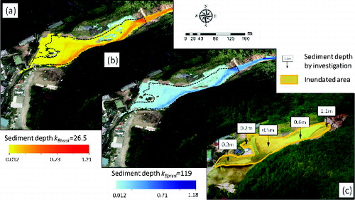
In addition, for prediction, the mobility coefficient can be computed as (29) where S_f and S_c are the slope gradient of fan and channel, respectively. Recommended value of S_f is 1.02 and S_c equals tan (9°), consequently k_Bpred should be 111.9, it is 4.3 times larger than k_Bback. It should be noticed that different values of k should make different inundated regions on the fan. However, figure 11(b) indicates that the area of inundated region simulated by k_Bpred increases little with the mobility coefficient k. It implies that TopFlowDF would like to inundate a bigger area but because the perimeter is too small that the simulation stops. In other words, the assumed area controlled by k is not reached when the simulation stops, so that the simulation based on different k shows no differences.

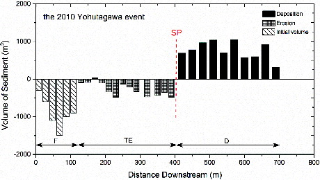
Compared to the post-hazard investigation (figure 11(c)), simulated deposition pattern by both back-analysis and prediction shows a good agreement with the investigation result, as well as the sediment depth and run-out distance. Calculated and simulated distribution of sediment volume in initial, erosion and deposition regions is also shown in figure 12.

Figure 12. Distribution of mass volume in the 2010 Yohutagawa debris-flow event.

6. Discussions

One limitation of this approach is the assumption of constant material strength of bed sediment, because the spatial and temporal variation of these parameters may exist and somewhat influence the theoretical results. Iverson et al. (1998) suggested the use of simplified spatially distributed models based on empirical or semi-empirical approaches, because these varying parameters cannot be acquired for a whole erosion region at reasonable cost, this view was also accepted by the researchers, e.g. Carrara et al. (2008), Horton et al. (2013). We have to advise in situ surveys and geotechnical test to obtain a rational value of these parameters, or do some empirical calibration according to the typical value. However, it will make the approach not easily portable from one region to another. Our current work is focusing on the solution to this problem. We intend to combine this approach with Monte Carlo methods, that in one step, we generate a set of random values of the parameters within an appropriate extent, and can get a calculated result. Typically we repeat this procedure many times over, and then obtain the distribution of the erosion depth and total volume. This will be further discussed.

Another limitation is the pore-pressure equation in equation (13). The described equation is under the conditions of the slope-parallel seepage, uniform flow and instant drainage. However the unsteady motion of debris flow may not allow these conditions to exist. A more realistic assumption was proposed by Sassa (1985) and Hungr et al. (2005), full bulk weight of debris-flow mass will be transferred to pore-water by undrained loading. But it will result in a too large erosion depth because the bed sediment may liquefy and become unstable naturally. This aspect still needs further discussion and evaluation.

7. Conclusions

In this paper, we present a new approach to estimate the sediment entrainment by the debris flows, which may provide a better solution to the input parameters of TopFlowDF model. The approach is derived from the static equilibrium of a three-layer model, and is further used to analyse the amplification of mass volume and peak discharge. Analysis indicates that topographic variables (slope of channel, top width of bed) influence the entrainment of the bed sediment. Based on it, a new concept of critical line is proposed, which is capable to detect the entrainment reaches in the channel. Two previous debris-flow events are selected to illustrate the approach; analytical results show a good agreement with the in situ survey. The main limitation of this approach is the assumption of constant material strength of bed sediment, as the spatial and temporal variation is neglected. Besides, the pore-pressure equation, used in the derivation, still needs further discussion and evaluation.

Acknowledgements

The authors are grateful to all the collaborators who participated in this study, and particularly to Dr Scheidl for his kind permission and providing of TopRunDF, TopFlowDF source code.

Funding

This study received financial support from Kyushu University Interdisciplinary Programs in Education and Projects in Research Development. It was also supported by JSPS KAKENHI [grant number 22310113] and the Global Environment Research Found of Japan (S-8). These financial aids are gratefully acknowledged.

Appendix A. Notation

Pi	=	Probability value from central cell towards cell i
θi	=	Slope angle from central cell towards cell i(°)
θc	=	Slope angle of the debris-flow channel (°)
Si	=	Accumulated probability from central cell towards cell i
naffect	=	Number of debris-flow trajectories that invade a cell
niteration	=	Total number of Monte Carlo iterations
U	=	Driving component of debris-flow mass
G	=	Resistance component
v	=	Velocity of the debris flow (m/s)
h	=	Flow height of the debris-flow mass (m)
g	=	Gravity acceleration (m/s2)
z	=	Bed-sediment entrainment depth (m)
Sfric	=	Friction coefficient of debris flow
τ	=	Shearing strength along the potential failure (kN)
τd	=	Shearing force by debris flow at the surface of bed sediment (kN)
c	=	Cohesion at potential failure (kN)
σ	=	Normal stress at potential failure (kPa)
σh(y)	=	Horizontal normal stress at the depth y in bed sediment (kPa)
σv(y)	=	Vertical normal stress at the depth y in bed sediment (kPa)
φ	=	Internal friction angle at potential failure (°)
γd	=	Specific weight of debris-flow fluid
nc	=	Manning's roughness coefficient
a	=	Empirical constant to estimate the velocity
W	=	Weight of generic element in bed-sediment entrainment model (kN)
γ	=	Saturated specific weight of bed material (kN/m3)
b	=	Channel path width (m)
u	=	Pore pressure in the bed sediment (kN/m3)
R1	=	Basal resistance of the bed sediment (kN)
R2	=	Side resistance of the bed sediment (kN)
Fd	=	Tractive force on the surface of bed-sediment failure (kN)
K	=	The earth pressure coefficient
ΔV	=	Bed-sediment entrainment volume (m3)
V	=	Total volume of the debris flow (m3)
hcritical	=	Critical flow depth of the debris flow to provoke the entrainment (m)
Qcritical	=	Critical discharge of the debris flow to provoke the entrainment (m3/s)
Q	=	Peak discharge of the debris flow in the chosen event (m3/s)
M	=	Debris-flow volume in the chosen event (m3)
kBback	=	Mobility coefficient for back analysis
kBpred	=	Mobility coefficient for prediction
Bobs	=	Observed inundation area by the debris flow (m2)
Sf, Sc	=	Slope gradient of fan and channel, respectively

References

- Bagnold RA. 1966. An approach to the sediment transport problem form general physics: physiographic and hydraulic studies. ( USGS Professional Paper 442-I).
- Blijenberg HM. 2007. Application of physical modelling of debris flow triggering to field conditions: limitations posed by boundary conditions. Eng Geol. 91:25–33.
- Brayshaw D, Hassan MA. 2009. Debris flow initiation and sediment recharge in gullies. Geomorphology. 109:122–131.
- Breien H, De Blasio FV, Elverhøi A, Høeg K. 2008. Erosion and morphology of a debris flow caused by a glacial lake outburst flood, Western Norway. Landslides. 5:271–280.
- Carrara A, Crosta G, Frattini P. 2008. Comparing models of debris-flow susceptibility in the alpine environment. Geomorphology. 94:353–378.
- Cenderelli DA, Kite JS. 1998. Geomorphic effects of large debris flows on channel morphology at North Fork Mountain, Eastern West Virginia, USA. Earth Surface Processes Landforms. 23:1–19.
- Chen GQ. 2008. Practical techniques for risk analysis of earthquake-induced landslide. Chin J Rock Mech Eng. 27:2395–2402.
- Chen H, Crosta GB, Lee CF. 2006. Erosional effects on runout of fast landslides, debris flows and avalanches: a numerical investigation. Géotechnique. 56:305–322.
- Chen J, He YP, Wei FQ. 2005. Debris flow erosion and deposition in Jiangjia Gully, Yunan, China. Environ Geol. 48:771–777.
- Chen NS, Yue ZQ, Cui P, Li ZL. 2007. A rational method for estimating maximum discharge of a landslide-induced debris flow: a case study from southwestern China. Geomorphology. 84:44–58.
- Chen YC, Yu FC. 2011. Morphometric analysis of debris flows and their source areas using GIS. Geomorphology. 129:387–397.
- Christen M, Kowalshi J, Bartelt P. 2010. RAMMS: numerical simulation of dense snow avalanches in three-dimensional terrain. Cold Region Sci Technol. 63:1–14.
- Duzgun HSB, Yucemen MS, Karpuz C. 2002. A probabilistic model for the assessment of uncertainties in the shear strength of rock discontinuities. Int J Rock Mech Mining Sci. 39:743–754.
- Gamma P. 2000. dfwalk – a debris flow simulation program for hazard zonation. Geographic Bernesia. G66, Bern. German.
- Glade T. 2005. Linking debris-flow hazard assessments with geomorphology. Geomorphology. 66:189–213.
- Han Z, Chen GQ, Li YG, Xu LR, Zheng L, Zhang YB. 2014. A new approach for analyzing the velocity distribution of debris flows at typical cross-sections. Nat Hazards. doi:10.1007/s11069-014-1276-3
- Han Z, Xu L, Su ZM, Wu Q. 2012. Research on lateral distribution features of debris flow velocity and structural optimization of prevention and control works. Rock Soil Mech. 33:3715–3720. Chinese.
- He SM, Wu Y, Li XP. 2007. Research on eroded start mechanism of channel debris flow. Rock Soil Mech. 28:155–159.
- Horton P, Jaboyedoff M, Rudaz B, Zimmermann M. 2013. Flow-R, a model for susceptibility mapping of debris flows and other gravitational hazards at a regional scale. Nat Hazards Earth Syst Sci. 13:869–885.
- Huber A. 2012. Implication for practical model application to hazard assessment for alpine transport infrastructure. 12th Congress Interpraevent 2012. Grenoble, France; p. 176–177.
- Hungr O, Mcdougall S. 2009. Two numerical models for landslide dynamic analysis. Comput Geosci. 35:978–992.
- Hungr O, Mcdougall S, Bovis M. 2005. Entrainment of material by debris flow. In: Jakob M, Hungr O, editors. Debris-flow hazards and related phenomena. Berlin: Springer; p. 136–137.
- Hungr O, Morgan G, Kellerhals R. 1984. Quantitative analysis of debris torrent hazards for design of remedial measures. Can Geotech J. 21:663–677.
- Hürlimann M, Rickenmann D, Medina V, Bateman A. 2008. Evaluation of approaches to calculate debris-flow parameters for hazard assessment. Eng Geol. 102:152–163.
- Iverson RM. 2012. Elementary theory of bed-sediment entrainment by debris flows and avalanches. J Geophys Res. 117:F03006.
- Iverson RM, Reid ME, Logan M, LaHusen RG, Godt JW, Griswold JG. 2011. Positive feedback and momentum growth during debris-flow entrainment of wet bed sediment. Nat Geosci. 19:116–121.
- Iverson RM, Schilling SP, Vallance JW. 1998. Objective delineation of lahar-inundation hazard zones. Geol Soc Am Bull. 110:972–984.
- Jaky J. 1944. The coefficient of earth pressure at rest. J Soc Hungarian Architects Eng. 78: 355–358. hungarian.
- King J. 1996. Tsing Shan debris flow. ( Special Project Report SPR 6/96). Hong Kong: Geotechnical Engineering Office, Hong Kong Government.
- Mangeney A. 2011. Landslide boost from entrainment. Nat Geosci. 4:77–78.
- Mangeney A, Tsimring LS, Volfson D, Aranson IS, Bouchut F. 2007. Avalanche mobility induced by the presence of an erodible bed and associated entrainment. Geophys Res Lett. 34:L22401.
- May CL, Gresswell RE. 2004. Spatial and temporal patterns of debris flow deposition in the Oregon Coast Range, USA. Geomorphology. 57:135–149.
- Medina V, Hürlimann M, Bateman A. 2008. Application of FLATModel, a 2D finite volume code, to debris flows in the northeastern part of the Iberian Peninsula. Landslides. 5:127–142.
- Mizuyama T, Kobashi S, Ou G. 1992. Prediction of debris flow peak discharge. Proceedings of the International Symposium Interpraevent; Bern, Switzerland, Bd. 4, p. 99–108.
- Morgenstern NR, Sangrey. 1978. Methods of slope stability analysis. In: Schuster RJ, Krizek RJ, editors. Landslides, analysis and control (special report 176). Washington (DC): Transportation Research Board, National Academy of Sciences; p. 155–171.
- O’Brien JD. 2006. FLO-2D user's manual, version 2006.01. Nutrioso (AZ): FLO Engineering.
- O’Brien JS, Julien PY, Fullerton WT. 1993. Two-dimensional water flood and mudflow simulation. J Hydraulic Eng ASCE. 119:244–261.
- Ocakuglu F, Gokceoglu C, Ercanoglu M. 2002. Dynamics of a complex mass movement triggered by heavy rainfall: a case study from NW Turkey. Geomorphology. 42:329–341.
- O’Callaghan JF, Mark DM. 1984. The extraction of drainage networks from digital elevation data. Comput Vis Graphics Image Process. 28:328–344.
- Pirulli M, Pastor M. 2012. Numerical study on the entrainment of bed material into rapid landslides. Géotechnique. 62:959–972.
- Prochaska AB, Santi PM, Higgins J, Cannon SH. 2008. Debris-flow runout predictions based on the average channel slope. Eng Geol. 98:29–40.
- Quinn P, Beven K, Chevallier P, Planchon O. 1991. The prediction of hill slope flow paths for distributed hydrological modelling using digital terrain models. Hydrol Process. 5:59–79.
- Rickenmann D. 1999. Empirical relationships for debris flows. Nat Hazards. 19:47–77.
- Rickenmann D. 2005. Runout prediction methods. In: Jakob M, Hungr O, editors. Debris-flow hazards and related phenomena. Berlin: Praxis Springer; p. 305–324.
- Sassa K. 1985. The mechanism of debris flows. In: Proceedings of the Eleventh International Conference on Soil Mechanics and Foundation Engineering. San Francisco; p. 1173–1176.
- Scheidl C, Rickenmann D. 2010. Empirical prediction of debris-flow mobility and deposition on fans. Earth Surf Proc Land. 35:157–173.
- Scheidl C, Rickenmann D. 2011. TopFlowDF – a simple GIS based model to simulate debris-flow runout on the fan. Italian J Eng Geol Environ. 30:253–261.
- Takahashi T. 1978. Mechanical characteristics of debris flow. J Hydr Div. 104:1153–1169.
- Takahashi T. 1991. Debris flow: IAHR monograph series. Rotterdam: Balkema.
- Takahashi T. 2007. Debris flow: mechanics, prediction and countermeasures. Leiden: Taylor & Francis.
- Takahashi T. 2009. A review of Japanese debris flow research. Int J Erosion Control Eng. 2:1–14.
- Tarboton DG. 1997. A new method for the determination of flow directions and upslope areas in grid digital elevation models. Water Resour Res. 33:309–319.
- Vasiliou A, Maris F, Varsami G. 2011. Estimation of sedimentation to the torrential sedimentation fan of the Dadia stream with the use of the TopRunDF and the GIS models. Adv Res Aquatic Environ. 1:207–214.
- Wang WL, Yen BC. 1974. Soil arching in slopes. J Eng Division. 1:61–78.
- Wu J, Chen G, Zheng L. 2013. GIS-based numerical simulation of Amamioshima debris flow in Japan. Front Struct Civ Eng. 12:1–9.