Evaluation of the dynamic processes of a landslide with laser scanners and Bayesian methods

Abstract

This paper deals with the study of the dynamics of a landslide from two different but complementary point of views. The landslide is situated within the Miozza basin, an area of approximately 10.7 km² located in the Alpine region of Carnia (Italy). In the first part of the paper, the macro-scale analysis of volumetric changes occurred after the reactivation of landslide in 2004 is addressed by using a two-epoch laser scanning surveys from airborne (ALS) and terrestrial (TLS) platforms. airborne laser scanning (ALS) data were collected in 2003 (before reactivation of the phenomenon) with an ALTM 3033 OPTECH sensor while terrestrial laser scanning (TLS) measurements were acquired in 2008 with a Riegl LMS-Z620. The second part of the paper deals with the study of dynamic processes of the landslide at micro-scale. To this aim, a global navigation satellite system (GNSS)-based monitoring network is analysed using a statistical approach to discriminate between measurement noise and possible actual displacements. This task is accomplished using both “classical” statistical testing and a Bayesian approach. The second method has been employed to verify some apparent vertical displacements detected by the classical test.

As regards the first topic of the paper, achieved results show that long-range TLS instruments can be profitably used in mountain areas to provide high-resolution digital terrain models (DTMs) with superior quality and detail with respect to aerial light detection and ranging data only, even in areas with very low accessibility. Moreover, ALS- and TLS-derived DTMs can be combined each other in order to fill gaps in ALS data, mainly due to the complexity of terrain morphology, and to perform quite accurate calculations of volume changes due to landslide phenomenon. Finally, the outcomes of the application of Bayesian inference demonstrate the effectiveness of this method to better detect statistically significant displacements of a GNSS monitoring network points. However, the application of this method in the geodetic field requires the identification of a preferring direction of displacements, what is not always feasible in advance.

1. Introduction

Slope collapses due to surface unstability are of particular interest for geomorphological studies, as they affect mainly the loose soil cover colluvium. Indeed, such phenomena are highly dangerous as they are liable to evolve into debris flows channelled by the engravings of lower order channels, affecting anthropogenic settlements such as buildings (Piragnolo et al. 2014) and road networks (Pirotti et al. 2011). The triggering factor is generally attributable to an extreme rainfall stream which penetrates the upper layers of the soil, but is not as much quickly drained by the deeper and less permeable parts or through the bedrock. The unstable material is subsequently transferred, at least partially, in the channel network and increases solid transport, affecting the temporal dynamics of the propagation of the sediment along the drainage network and also the morphology of the riverbed. The ability to identify a higher or lower susceptibility degree of the slope of a river basin is, therefore, of particular interest not only for a correct evaluation of the budget of the sediments at the basin scale (Brardinoni et al. 2011; Larsen 2012; Chang et al. 2014) but also for risk-prevention policies (Guzzetti 2003; Giulivo et al. 2013; Scolobig et al. 2014).

Besides traditional surveying methods (GNSS, robotic total station, boreholes, inclinometers, TDR, etc.), the use of modern remote sensing techniques for landslide investigations and monitoring has exponentially grown in recent years. Unmanned aerial vehicles are capable of carrying out surveys “on demand” with relative high accuracy (Coppa et al. 2009) using photogrammetry and in near future also light detection and ranging (LiDAR). Ground-based interferometric synthetic aperture radar (GBSAR) and LiDAR techniques allow for the production of highly detailed and accurate digital terrain models (DTMs). This fact has opened new way of applications for the study of landslide phenomena. In this field, GBSAR-based systems are mainly used for the detection and quantification of small displacements over large areas (Recife et al. 2000; Xia et al. 2004; Schulz et al. 2012; Crosetto et al. 2013; Jebur et al. 2014a). LiDAR sensors, based on aerial and terrestrial platforms, provide high-resolution sampling of the terrain surface in the form of very dense point clouds, operating over areas of variable extent. In particular, terrestrial laser scanners (TLSs) allow to acquire huge data-sets with high resolution in a very short time, from which a precise and detailed description of the scanned area can be derived (Slob & Hack 2004; Heritage & Large 2009; Shan & Toth 2009; Vosselmann & Maas 2010). As illustrated in Jaboyedoff et al. (2012), main applications of LiDAR technologies to landslide studies range from mapping and characterization (Ardizzone et al. 2007; Derron & Jaboyedoff 2010; Guzzetti et al. 2012; Jebur et al. 2014b) to monitoring (Teza et al. 2007; Oppikofer et al. 2008; Abellan et al. 2009, 2010; Prokop & Panholzer 2009; Barbarella & Fiani 2013). GBSAR and TLS techniques can also be used in combined way in order to improve the understanding of landslide phenomena, as is described in Lingua et al. (2008) and Teza et al. (2008). The introduction in 2004 of ALS systems with echo digitization and full waveform analysis (FWA) capabilities (Hug et al. 2004; Wagner et al. 2004) has definitely led to significant improvements to aerial LiDAR data processing in multi-target environments (Pirotti et al. 2013). In particular, data classification, vegetation filtering, surface model extraction and radiometric measurements have greatly benefited from these advances (Pirotti 2011; Ullrich et al. 2007; Wagner 2010). In addition to FWA based on digitized and stored echo signals in off-line processing of ALS data, Riegl Company has introduced in 2008 a new series of commercial scanning systems, the V-Line (Pfennigbauer & Ullrich 2010), also offering echo digitization. Unlike airborne systems, the V-Line laser scanners use online waveform processing, yielding similar results compared to full waveform analysis with even higher accuracy and precision, but with limitations with regard to multi-target resolution (Ullrich & Pfennigbauer 2011). Given this additional processing feature, it is advisable that in next future, airborne and terrestrial LiDAR systems will be increasingly used for landslide investigations even in densely forested areas. By exploiting echo discrimination capability of waveform systems, data processing time (e.g. vegetation filtering) can be greatly reduced, and more reliable and accurate DTMs can be derived from acquired data.

According to the Italian regulations, in case of a landslide event which can lead to potential hazard for human lives and settlements, two kinds of activities have to be undertaken. The first one operates at macro-scale level and is aimed at the assessment of the volumes (erosion and deposition) of debris material moved by the phenomenon. The second task works at micro-scale level and deals with the continuous monitoring of the area under investigation through a GNSS control network.

On the ground of these regulations, in the next sections, the application of LiDAR and GPS surveying techniques to the monitoring of a landslide in northern Italy will be discussed. Dynamic processes of this landslide have been, therefore, investigated both at macro-scale and micro-scale levels. The former analysis has dealt with the assessment of the amount of mass material mobilized after the reactivation of the landslide in 2004, due to a series of severe rainfall events. To this aim, DTMs derived from ALS and TLS surveys, performed in different epochs, were compared. Mass losses and deposition were estimated through a Cut & Fill volumetric analysis performed on the difference of DTMs (DoD). A GNSS-based geodetic network was also established around the main landslide body for monitoring purposes. The main goal of this activity is to detect surface changes at micro-scale level through multi-temporal surveys of the network. Deformation analysis can be carried out applying suitable movement significance tests or estimating deformation model parameters. Often these two procedures are adopted together. In both cases, usually suitable statistical methods are adopted to distinguish between actual displacements and random measurement errors. The most used methodologies to perform inferential tests are based on the “classical” frequentist approach and make use of the observations only (Caspary 2000; Koch 1999). On the other hand, when the estimated displacements are small with respect to the measurement precision, the classical testing procedure is not able to detect significant displacements even if they show an internal consistency, for instance when they show a common direction of movement (Albertella et al. 2006; Tanir et al. 2008; Betti et al. 2011). The Bayesian approach allows to account for all the available prior information on the phenomenon under examination, thus it can help to overcome the limit of classical testing. In this paper, both statistical approaches have been adopted in order to assess the stability of a set of GNSS network control points, to be used as references for subsequent monitoring activities of the landslide. Of course, to this aim further GNSS network points have to be arranged inside the landslide area. From the joint analysis of statistically significant displacements of such additional points and of the occurrence of severe rainfall events, an early warning system could be developed for the safety of the local population living at the bottom of the alpine basin within which the landslide is located.

2. The study area

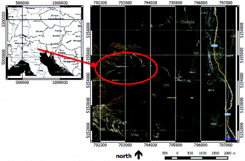
The study area considered in this work covers the head sub-basin of the Miozza catchment, a small basin of 4.4 km² located in Carnia, a tectonically active alpine region in the north-east of Italy (figure 1). Elevation ranges from 834 and 2075 m a.s.l, with an average value of 1530 m above sea level (a.s.l.) The slope angle has an average value of 34°, with a maximum of 74° at the head of the basin. No significant anthropic structures are present here and human activity is limited just to the cattle grazing. The area has a typical north-eastern Alpine climate with short dry periods and a mean annual precipitation of about 2200 mm. This is one of the most rainy areas of Italy. Precipitation occurs mainly as snowfall from November to April; run-off is usually dominated by snowmelt in May and June. During the most intense weather events such as floods, debris flows and channel slope, instability processes are common. Vegetation covers 91% of the area and consists of forest stands (64%), shrubs (19%) and mountain grassland (17%); the remaining 9% of the area is un-vegetated landslide scars (8%) and bedrock outcrops (1%). The geomorphologic setting of the basin is typical of the eastern alpine region, with deeply incised valleys. Soil thickness varies between 0.1 and 0.5 m on topographic spurs and depths of up to 1.5 m in topographic hollows.

Figure 1. Geographic location of the Miozza basin (WGS84/UTM32 coordinate reference system).

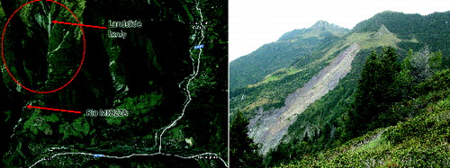
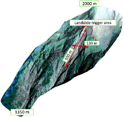
The basin was chosen as study area primarily because it is representative of the lithological and physiographical conditions frequently observed in the Carnia region where the mapping of landslide impacts is of interest. Furthermore, detailed information on topography, channel network, land use and geomorphology from different sources (including airborne LiDAR) were available (Tarolli & Tarboton 2006; Tarolli & Dalla Fontana 2008). Most of the instability areas are located at the head of the basin and result from the aggregation of many shallow landslides. The largest single landslide section, covering an extent of 0.27 km² (figure 2), is the most active and the main source of triggering of debris-flows which propagate along the main shaft, almost to the closing section of the basin. The most significant landslide event occurred around the months of March/April 2004, and it has mobilized a considerable amount of silt-clay material as a result of increased water flow due to the seasonal snow melting. The debris covered the bed of the river for several hundred meters.

Figure 2. (Left) The Miozza basin in Carnia, the study area is marked by the red circle. (Right) Side view of the main landslide body. To view this figure in colour, please see the online version of the journal.

3. Macro-scale analysis

From sequential monitoring over time, the volume of registered collapses of a slope can be deduced and the landslide movement along the main geological structures can be inferred. To achieve these objectives, the main body of the landslide under investigation was surveyed with aerial and terrestrial LiDAR systems in two subsequent epochs. A DoD was derived by comparing the corresponding DTMs and deposition and erosion volumes were estimated, as described in following sub-sections.

3.1. ALS data acquisition

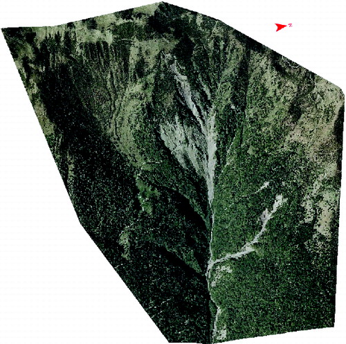
In November 2003, before the reactivation of the main landslide body, the whole area was monitored with a helicopter-based LiDAR system within the project INTERREG IIIA Italy-Slovenia. The survey was performed in snow-free conditions using an ALTM 3033 OPTECH sensor and an on-board Rollei H20 digital camera (Shan & Toth 2009). At a flight height of 1000 m, an average point density of 2 points/m² was acquired, recording the first, intermediate and the last returns. Vegetation was then properly filtered out from the ALS data in order to keep just the bare terrain, and a detailed DTM of the whole basin was generated in ArcGIS. Finally, orthophotos derived from digital images were draped on the DTM (figure 3).

Figure 3. The DTM derived from 2003 LiDAR flight. On the middle the main landslide body while on the right the results of some minor slope collapses.

3.2. TLS data acquisition

As already mentioned in Section 3, in 2004 a series of severe rainfall events triggered a significant movement of the main landslide. A further survey was, therefore, scheduled in order to estimate the amount of material globally moved by such events. In this case, however, it was decided to employ a long-range TLS instead of performing a more expensive LiDAR flight. The primary objective of this approach was to evaluate the potential and the benefit of very high resolution TLS-derived DTMs, compared to those from airborne LiDAR, for landslide modelling applications in alpine environment.

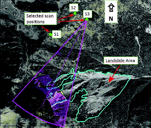
The presence of very steep slopes in the area under study (up to 74° at the head of the basin) and difficulties met during previous measurement campaigns, aimed to rainfall data collection and monitoring of current state of the hydrographic basin, highlighted the need for a careful planning of the survey with a TLS. The main goal of this step was to roughly identify on the map the best positions where to set up the laser stations. Based on the 2003 LiDAR DTM, a visibility analysis was, therefore, carried out in ArcGIS, taking into account terrain morphology, logistics (roads and pathways) and safety conditions (via raster of slopes and photographs of the area). Through the visibility map, three potential laser stations (S1, S2 and S3 in figure 4) were identified, with a stand-off distance from the area of interest varying between 800 and 1500 m. In order to operate over these long distances, a Riegl LMS-Z620 (Riegl 2014), owned by Cirgeo, was employed. At the time of the survey, the Z620 was the first available TLS on the market offering a maximum range up to 2000 m in combination with high accuracy and high speed data acquisition.

Figure 4. Visibility map created in ArcGIS on the LiDAR-derived DTM, showing the planned scan positions (green points), an example of the visibility cone (purple lines) and the perimeter of the whole landslide body (blue line). To view this figure in colour, please see the online version of the journal.

The survey was realized in spring 2008 after the snow-melting period. Scans were acquired from a laser station close to the candidate point S3; the maximum object-distance from the scanner was around 1200 m (figure 5(a)). Small clouds climbing up from the bottom of the landslide, which were absorbing the laser beam, and residuals of night moisture on the rocks hindered the data acquisition. The actual working time was, therefore, limited to a quite narrow window spanning from 11 am to 3 pm, after that the survey was stopped because of increasing rainfall risk. The TLS data processing was completely performed within RiSCAN PRO, the companion software to Riegl 3D TLSs. Firstly, the vegetation was removed from acquired scans by semi-automatic filtering procedures, then the resulting DTM was georeferenced through the so-called backsight orientation approach. To this aim, the position of the laser station and that of a retro-reflective target, placed in the nearby (figure 5(b)), were measured with two Topcon Hiper Pro double frequency GNSS receivers (Topcon 2014a). The sets of static observations acquired from both positions were then corrected in post-processing within the software TopconTools (Topcon 2014b). To this aim, two baselines with the closest GNSS permanent station of the Friuli Regional Deformation Network (FReDNet 2014) were determined. This is a regional network comprising of 11 permanent stations, which provides real-time corrections for Real Time Kinematic positioning and raw measurements (receiver independent exchange format [RINEX] data) for post-processing of static and fast-static GNSS surveys. After this step, the laser station and target positions were estimated with a horizontal accuracy of 5 mm and a vertical accuracy of 1 cm. All in all, considering that errors affecting TLS measurements (Lichti & Gordon 2004; Scaioni 2005) are dominated in the present case by uncertainty of georeferencing procedure and range determination, the accuracy of the acquired laser point cloud can be assessed at the level of a few centimetres (<10 cm).

Figure 6 shows the resulting high resolution DTM (HRDTM) of 25 cm × 25 cm textured with the images captured by the mounted calibrated camera, Nikon D90. The landslide triggered by 2008 rainfall events was covering an area of around 650 m in vertical direction and 130 m in horizontal direction.

Figure 5. (Left) The Riegl LMS-Z620 with the mounted Nikon D90 digital camera and the Topcon Hiper Pro GNSS receiver on top. (Right) The retro-reflective target used for the back-sight orientation of the scan position.

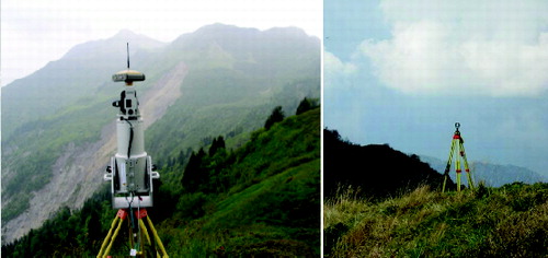
Figure 6. The HRDTM derived from TLS data.

3.3. Volumetric analysis

After the GNSS data processing, the TLS-derived DTM was georeferenced in RiSCAN PRO software, through the backsight orientation procedure, within the ETRF2000 reference frame. Since the 2003 LiDAR DTM was referred to the ETRF89 frame, in order to eliminate potential systematic errors due to the shifts between these two frames, a further global registration was applied to both DTMs. The automatic alignment procedure was calculated by the multi-station-adjustment (MSA) plugin of RiSCAN PRO, using common points located in overlapping areas, outside of the landslide perimeter.

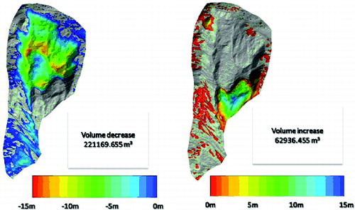
Once the two data-sets were registered to each other, the mass balance could be calculated. The results of Cut & Fill volume analysis are illustrated in figure 7 on the DTM derived from the TLS data. The volumetric comparison showed a massive material loss in the upper part of the landslide (about 221.000 m³, left side of figure 7) and a partial deposition in the lower areas (about 63.000 m³, right side of figure 7). A comparable result was obtained in a previous study conducted in the same area by computing volumetric differences between airborne LiDAR-derived DTMs (Massari et al. 2007) acquired before and after landslide activity.

Figure 7. Results of the Cut & Fill volumetric analysis performed between the 2003 LiDAR- and 2008 TLS-derived DTMs.

4. Analysis of micro-scale displacements

At the same time as the TLS survey, a GNSS control network was also established around the whole landslide area in order to determine slow surface movements. In order to evaluate the stability over time of the five network points, two statistical analyses have been applied: one based on classical inference and a second based on Bayesian inference. While the former is aimed at the estimate of point displacements due to surface instability phenomena, the Bayesian approach allows to identify in advance the areas on the ground with statistically significant shifts. A drawback of traditional statistical methods is that they work well only when point displacements between different survey epochs are sufficiently large compared to the standard deviations of related coordinates. In such cases, coordinate differences of some points can be marked as potential displacements by the classical methods. The Bayesian analysis can help to better discriminate these “ambiguities”. As will be described in next Section 4.1, point shifts computed with respect to the first measurement epoch were at the same order of magnitude as the uncertainties of corresponding coordinates. After the application of the classical statistical test, two network points, close to the landslide area, seemed to be unstable. Therefore, in order to remove or validate the hypothesis of instability, the Bayesian statistical inference was applied.

4.1. The GNSS control network

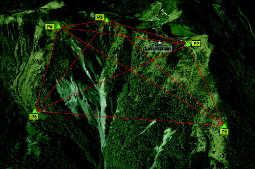
As for the TLS survey, the location of the set of potentially stable control points was detected using the 2003 LiDAR DTM and taking into account the terrain morphology, logistics and safety (slopes steepness) issues (Wang & Soler 2012). In order to determine the best set of candidate locations, several sky-plots were realized. Information about potential obstructions (mainly due to vegetation and rocks) was derived from the 2003 LiDAR DSM. Five benchmarks were then selected and properly monumented in the field by cementing steel survey nails into the ground or into the rocks (figure 8). This solution was adopted in order to easily recover the marks in subsequent surveys and to prevent possible displacements due to the passing of local fauna or cattle. The length of all potential baselines of the resulting geodetic network was ranging between 500 m and 1.5 km. Six surveys have been globally performed from 2008 to 2010, with a six-month time interval: in May, after the snow-melting period, and in early October, before the winter season. For each measurement campaign, three independent static sessions were carried out in order to observe all the independent baselines (10) allowed by the network geometry. Station occupation time was set to one hour with a sampling rate of 10 s. For the data collection, the following geodetic-grade GNSS receivers were employed; two Topcon HiPer Pro, a Leica Wild GPS System 200 with SR299 antenna and a Trimble 5700. A minimal constraints network adjustment was then separately applied to each acquired data-set, using all available independent baselines. The computations have been performed in TopconTools software adopting the “single base” approach. For each adjustment run, the coordinates of point P1 were kept fixed, being this one the point located in the most geological stable location in the neighbourhood of the landslide. Preliminary loop closure analysis of the post-processed baselines showed all the times misclosures of a few millimetres, thus denoting the absence of any gross error in the observations. The resulting adjusted coordinates (N, E, h) of the five control points are listed in table 1. Here, the differences (ΔE, ΔN, Δh) have been computed with respect to the first survey epoch. Adjustment of the geodetic network yielded coordinate standard deviations at centimetre level.

Table 1. Results of the GNSS network adjustment. Point coordinates (N, E, h) are listed according to the measurement campaign (1 = May, 2 = October) and survey year.

Point	Year	Meas. camp.	E (m)	N (m)	h (m)	ΔE (m)	ΔN (m)	Δh (m)
P1	2008	1	332,827.971	5,150,633.015	1654.414	−	−	−
		2	332,827.960	5,150,633.020	1654.406	0.011	0.005	0.008
	2009	3	332,827.954	5,150,633.022	1654.404	0.017	0.007	0.010
		4	332,827.955	5,150,633.027	1654.385	0.016	0.012	0.029
	2010	5	332,827.963	5,150,633.021	1654.406	0.008	0.006	0.018
		6	332,827.966	5,150,633.024	1654.389	0.005	0.009	0.025
P2	2008	1	332,000.389	5,150,550.547	1876.640	−	−	−
		2	332,000.395	5,150,550.539	1876.655	0.006	0.008	0.015
	2009	3	332,000.403	5,150,550.536	1876.627	0.014	0.011	0.013
		4	332,000.407	5,150,550.526	1876.616	0.018	0.021	0.024
	2010	5	332,000.401	5,150,550.532	1876.620	0.012	0.015	0.020
		6	332,000.394	5,150,550.534	1876.623	0.005	0.013	0.017
P3	2008	1	331,442.312	5,149,844.482	1857.293	−	−	−
		2	331,442.322	5,149,844.488	1857.281	0.010	0.006	0.012
	2009	3	331,442.331	5,149,844.495	1857.262	0.019	0.013	0.031
		4	331,442.331	5,149,844.502	1857.265	0.019	0.020	0.028
	2010	5	331,442.334	5,149,844.496	1857.259	0.022	0.014	0.034
		6	331,442.328	5,149,844.506	1857.264	0.016	0.024	0.029
P4	2008	1	331,560.049	5,149,365.421	1887.066	−	−	−
		2	331,560.038	5,149,365.411	1886.884	0.011	0.010	0.182
	2009	3	331,560.074	5,149,365.452	1887.169	0.025	0.031	0.103
		4	331,560.090	5,149,365.447	1887.049	0.041	0.026	0.017
	2010	5	331,560.081	5149365.436	1887.025	0.032	0.015	0.041
		6	331560.088	5,149,365.464	1887.892	0.039	0.043	0.174
P5	2008	1	332,377.745	5,149,162.943	1466.324	−	−	−
		2	332,377.757	5,149,162.962	1466.303	0.012	0.019	0.021
	2009	3	332,377.771	5,149,162.968	1466.192	0.026	0.025	0.132
		4	332,377.779	5,149,162.971	1466.282	0.034	0.028	0.042
	2010	5	332,377.762	5,149,162.970	1466.168	0.017	0.027	0.156
		6	332,377.774	5,149,162.966	1466.291	0.029	0.023	0.033

Figure 8. The GNSS control network.

4.2. Statistical analysis of displacements with the classical method

In this approach, the coordinates (N, E, h) of each control point P_j (j = 1, … , 5) have been analysed separately. It has also been assumed that no spatial and time correlations did exist between such coordinates.

Denoting with , the displacement between adjusted coordinates x₁ and x₂ of homologous points, derived from surveys conducted at epochs t₁ and t₂, the presence of unavoidable residual errors v_i in the least-squares estimate of each parameter x_i (i = 1, … 6) leads to consider the following relationship: (1) where Δx is a random variable with normal distribution of unknown mean δx and known variance , (2)

The magnitudes and are known as they have been calculated by the least-squares network adjustment at the two surveying epochs t₁ and t₂. In order to statistically check the significance of the network point displacements, computed within the six surveys, the null hypothesis tested was that no significant displacements occurred between two measurement epochs. Therefore, (3) (4)

The test statistics adopted in this analysis was the well-known standardized random variable Z, with (5)

The acceptance region of the null hypothesis H₀ was therefore: (6) with a significance level α = 5% and a critical value (two-tailed test).

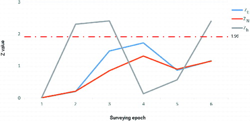
Results of statistical testing are illustrated in the following tables 2–4. The Z-values have been calculated according to equation (5), assuming as reference positions for the displacements Δx those of the network points at the first surveying epoch.

Table 2. Z values of the east coordinate for each control point. Displacements ΔE are computed with respect to the first surveying epoch.

	2 → 1	3 → 1	4 → 1	5 → 1	6 → 1
P1	0.25	0.20	0.61	0.54	0.36
P2	0.13	0.36	0.78	1.27	1.30
P3	0.18	0.24	0.38	0.65	0.90
P4	0.20	1.46	1.72	0.87	1.16
P5	0.46	1.47	0.93	1.52	0.73

Table 3. Z values of the north coordinate for each control point. Displacements ΔN are computed with respect to the first surveying epoch.

	2 → 1	3 → 1	4 → 1	5 → 1	6 → 1
P1	0.70	0.17	1.55	0.31	0.80
P2	0.49	0.35	1.12	0.91	1.51
P3	0.81	0.68	0.99	0.92	1.15
P4	0.21	0.85	1.31	0.90	1.15
P5	0.35	0.61	0.61	1.70	1.48

Table 4. Z values of the h coordinate for each control point. Displacements Δh are computed with respect to the first surveying epoch. Shaded cells show the cases where the null hypothesis H₀ has been rejected.

	2 → 1	3 → 1	4 → 1	5 → 1	6 → 1
P1	0.15	1.23	1.07	0.55	0.70
P2	0.29	1.12	1.61	1.65	1.50
P3	0.75	0.64	1.24	0.99	1.49
P4	2.13	2.13	0.13	0.57	2.40
P5	0.51	2.08	0.34	2.15	1.12

As shown in tables 2 and 3, no significant horizontal displacements occurred between 2008 and 2010: all the observed values Z_E and Z_N are indeed below the defined threshold value (1.96). Conversely, potential instability conditions were likely to affect the vertical component of points P4 and P5, as highlighted by the cells in green colour in table 4. A plot of the computed Z_N, Z_E and Z_h values for point P4 is illustrated in figure 9.

Figure 9. Z values of N, E, h coordinates for the point P4 obtained from the statistical classical analysis.

4.3. Analysis of displacements with the Bayesian method

In order to evaluate whether the results obtained from classical analysis for the vertical component of points P4 and P5 denoted actual displacements or they were more likely due to residual random errors, a further statistical test based on Bayesian method was applied. The test was limited to the one-dimensional case since the results of classical analysis did not show any “ambiguity” on the horizontal components of the geodetic network points. Thus, for each point P_j the shifts Δh between different measurement campaigns were taken into account: (7)

In equation (7), h_i denotes the adjusted height of point P_j at surveying epoch t_i, while h₁ is the adjusted height of the same point at the first measurement epoch t₁, considered as reference value. Assuming that the shifts Δh have a normal distribution with unknown mean δh and known variance (computed from network adjustment), for each control point P_j the shift Δh can be written as: (8)

The mean δh is, in turn, a random variable following a normal distribution with mean μ and variance , which represents, in this analysis, the prior distribution of the Bayesian statistical inference. The parameters μ and are the prior information whose values have to be somehow set in advance.

Since the points P3, P4 and P5 were placed close to the landslide area, it is reasonable to assume that the vertical displacements are zero or, at the most, facing downwards. Therefore, considering an axis properly oriented, the following additional a-priori constraint has been set: (9)

Considering the observables Δh as dependant on parameter δh, the Bayes formula becomes (10)

All the terms on the right side of equation (10) can be explicitly calculated. The function f(δh) in this analysis denotes the a-priori probability distribution of parameters δh. This distribution follows a modified version of a normal distribution: along the negative semi-axis it is null, being the probability of the interval [−∞, 0] all concentrated in the origin, i.e. P₀ ≡ P{δh ≤ 0}. Given this constraint, the probability distribution of δh becomes (11) where θ(δh) is the Heaviside step function (12) and δ(δh) is the delta of Dirac function.

The value of P₀ can be calculated by considering the normalization condition applied to the distribution probability f(δh). Indeed, from equation (13) (13) it follows that (14)

The integral on the right side of equation (14) can be solved using the error function (Zwillinger 2012), whose values are available in specific tables: (15)

In this way, after a variable change, equation (14) becomes (16)

In equation (10), the function f(Δh|δh) can be regarded as the likelihood function L(Δh|δh) of variable Δh: (17)

The denominator of equation (10) is a normalization constant which can be numerically estimated. After some mathematical steps, the following formula is obtained: (18) with (19) and (20)

Being all terms in equation (10) defined in explicit form, the Bayes formula can be now numerically evaluated as follows: (21)

The benefit of using the two quantities A and B becomes clear by evaluating the probability that significant (δh ≥ 0) or not significant (δh = 0) vertical displacements have occurred between 2008 and 2010. Indeed, this operation is turned into the calculation of the following simple ratios: (22) (23)

The significance analysis of displacements through the Bayesian approach is thus reduced to a comparison between the two quantities (22) and (23). A probabilistic analysis can be, therefore, performed in place of a statistical testing. The result of the comparison allows to assess which of the two alternatives (significant or not significant shift) is more likely to be occurred.

While in the classical analysis a decision rule based on a confidence level α = 5% was used, in the Bayesian statistical analysis a different approach was adopted, as shown in table 5.

Table 5. Decision rules for the Bayesian statistical analysis.

P(δh > 0|Δh)	Decision rule
<0.475	Point displacement is not significant → P(δh = 0|Δh) > 0.525
>0.525	Point displacement is significant → P(δh = 0|Δh) < 0.475
0.475 ÷ 0.525	No assessment can be made about the significance of the displacement

Three tests were then carried out with different settings for the prior values of parameters μ and σ₀. For each test, the probabilities P(δh > 0|Δh) were calculated, assuming as reference for the comparisons the adjusted heights of the network points derived from the first measurement epoch. Although the classical analysis had highlighted some “ambiguities” just for points P4 and P5, the Bayesian approach was applied to all the control points. Test results are illustrated in tables 6–8. In the third test, the value of the parameter μ was set equal to the mean shift Δh for each point P_j.

Table 6. Results of Bayesian analysis with μ = 0.040 m and σ₀ = 0.02 m.

	2 → 1	3 → 1	4 → 1	5 → 1	6 → 1
P1	0.120	0.011	0.015	0.032	0.025
P2	0.060	0.015	0.007	0.002	0.030
P3	0.015	0.032	0.009	0.015	0.010
P4	0.011	0.035	0.098	0.056	0.042
P5	0.062	0.219	0.030	0.048	0.005

Table 7. Results of Bayesian analysis with μ = 0.050 m and σ₀ = 0.05 m.

	2 → 1	3 → 1	4 → 1	5 → 1	6 → 1
P1	0.250	0.003	0.003	0.073	0.025
P2	0.150	0.002	0.002	0.000	0.005
P3	0.020	0.030	0.001	0.005	0.002
P4	0.051	0.217	0.310	0.045	0.299
P5	0.058	0.368	0.017	0.139	0.030

Table 8. Results of Bayesian analysis with μ = variable and σ₀ = 0.08 m.

	2 → 1	3 → 1	4 → 1	5 → 1	6 → 1
P1	0.215	0.001	0.001	0.037	0.011
P2	0.045	0.000	0.000	0.000	0.002
P3	0.003	0.005	0.000	0.000	0.000
P4	0.007	0.022	0.100	0.004	0.031
P5	0.017	0.290	0.006	0.042	0.002

The data prior (μ, σ₀) were set according to the accumulated experience and knowledge about the landslide, derived from previous surveys. Results of the Bayesian approach clearly show that vertical displacements occurred in the time span 2008–2010 are “not significant”. Any doubt raised after the application of classical statistical analysis has thus been removed. The five control points P1, P2, P3, P4 and P5 of the geodetic network can be, therefore, denoted as “stable” in time, and they can be used as reference in further surveys aimed to evaluate landslide displacements at micro-scale level.

5. Conclusions

According to the Italian regulations for landslide monitoring, in this paper two complementary surveying methods have been presented. The first one operates at macro-scale level and is aimed at the assessment of the volumes (erosion and deposition) of debris material moved by the phenomenon. For this objective, laser scanning technology (based on both aerial and terrestrial platforms) has been used, as it allows to reconstruct the whole terrain surface. The second method works at micro-scale level and is based on the monitoring of the area under investigation through a GNSS control network. Unlike laser scanning technique, the GNSS-based approach involves a limited set of well-established points, whose displacements (if any) are estimated by comparing multi-temporal data-sets. Long and repeated baseline observations potentially allow to detect point shifts with millimetre order of magnitude.

The results obtained in the volumetric analysis of the Miozza landslide show the high potential of terrestrial laser scanning technology for the recovery of three-dimensional models useful for the monitoring of slopes subjected to hydro-geological instability. As highlighted in the first part of this work, the benefits of ALS- and TLS-based surveys can be summarized as follows:

1. Long-range TLS instruments can be profitably used in mountain areas to provide HRDTMs with superior quality and detail with respect to aerial LiDAR data only, even in areas with very low accessibility. The drawback of this approach relies in the limited extent of the area that can be surveyed at once.

2. The detail richness potentially achievable with a TLS system allows to extract additional information with respect to LiDAR data and thus to improve the analysis and modelling of small landslides areas.

3. ALS and TLS DTMs can be combined each other in order to fill gaps in ALS data, mainly due to the complexity of terrain morphology. In areas of low accessibility for ALS sensors, TLSs can be operated in a more flexible and profitable way, allowing to survey the same object from different scan positions. Thus, the scanning geometry can be improved by reducing the potential sources of obstructions to the laser beam, and a more complete DTM can be obtained.

As regards the study of Miozza landslide at the level of micro-scale displacements, the Bayesian statistical inference has confirmed the hypothesis of stability of the geodetic network points, surveyed with GNSS receivers between 2008 and 2010. This kind of analysis has also allowed to remove the doubts about any potential instability of two control points (P4 and P5), raised after the application of the classical statistical inference to the adjusted coordinates of the GNSS network. Traditional statistical methods, indeed, work well only when point shifts between different survey epochs are sufficiently large compared to the standard deviations of related coordinates. Although the Bayesian method should not be considered a substitute to the classic approach, as it uses a least squares estimate of the statistical parameters, nevertheless it is proposed as a useful tool for eliminating, or at least reducing, residual doubts derived from classical analysis. However, the application of the Bayesian statistical inference in the geodetic field requires the identification of a preferring direction of displacements, what is not always feasible in advance.

References

- Abellan A, Jaboyedoff M, Oppikofer T, Vilaplana JM. 2009. Detection of millimetric deformation using a terrestrial laser scanner: experiment and application to a rockfall event. Nat Hazards Earth Syst Sci. 9:365–372.
- Abellan A, Vilaplana JM, Calvet J, Blanchard J. 2010. Detection and spatial prediction of rockfalls by means of terrestrial laser scanning modelling. Geomorphology. 119:162–171.
- Albertella A, Cazzaniga N, Sansò F, Sacerdote F, Crespi M, Luzietti L. 2006. Deformations detection by a Bayesian approach: prior information representation and testing criteria definition. In: Sansò F, Gil AJ, editors. Geodetic deformation monitoring: from geophysical to engineering roles, IAG Symposia. Vol 131. Berlin: Springer; p. 30–37.
- Ardizzone F, Cardinali M, Galli M, Guzzetti F, Reichenbach P. 2007. Identification and mapping of recent rainfall-induced landslides using elevation data collected by airborne Lidar. Nat Hazards Earth Syst Sci. 7:637–650. doi:10.5194/nhess-7-637-2007
- Barbarella M, Fiani M, Lugli A. 2013. Application of LiDAR-derived DEM for detection of mass movements on a landslide. Int Arch Photogram Remote Sens Spat Inf Sci. XL-5/W3: 89–98. doi:10.5194/isprsarchives-XL-5-W3-89-2013
- Betti B, Cazzaniga NE, Tornatore V. 2011. Deformation assessment considering an a priori functional model in a Bayesian framework. J Surv Eng. 137:113–119. doi:10.1061/(ASCE)SU.1943-5428.0000052
- Brardinoni F, Crosta B, Cucchiaro S, Valbuzzi E, Frattini P. 2011. Landslide mobility and landslide sediment transfer in Val di Sole, Eastern Central Alps. Proceedings of the Second World Landslide Forum; 2011 Oct; Rome, Italy.
- Caspary WF. 2000. Concepts of network and deformation analysis, 3rd corrected impression. Sidney, Australia: University of New South Wales, School of Geomatic Engineering.
- Chang K-J, Huang Y-T, Huang M-J, Chiang Y-L, Yeh E-C, Chao Y-J. 2014. Sediment budget analysis from Landslide debris and river channel change during the extreme event – example of Typhoon Morakot at Laonong river, Taiwan. Geophys Res Abstr. 16:EGU2014–4844. EGU General Assembly.
- Coppa U, Guarnieri A, Pirotti F, Vettore A. 2009. Accuracy enhancement of unmanned helicopter positioning with low-cost system. Appl Geomatics. 1:85–95. doi:10.1007/s12518-009-0009-x
- Crosetto M, Gili JA, Monserrat O, Cuevas-González M, Corominas J, Serra D. 2013. Interferometric SAR monitoring of the Vallcebre landslide (Spain) using corner reflectors. Nat Hazards Earth Syst Sci. 13:923–933. doi:10.5194/nhess-13-923-2013
- Derron MH, Jaboyedoff M. 2010. Preface to the special issue. In: LIDAR and DEM techniques for landslides monitoring and characterization. Nat Hazards Earth Syst Sci. 10:1877–1879.
- FreDNet (Friuli Regional Network) [Internet]. 2014. Available from: http://www.crs.inogs.it/frednet/ItalianSite/XFReDNetHome.htm
- Giulivo I, Galluccio F, Matano F, Monti L, Terranova C. 2013. Landslide risk and mitigation policies in Campania region (Italy). In Margottini C., Canuti P., Sassa K., editors. Proceedings of the Second World Landslide Forum; Rome (Italy): Springer Berlin Heidelberg; p. 209–216. doi:10.1007/978-3-642-31313-4_27
- Guzzetti F. 2003. Landslide hazard assessment and risk evaluation: limits and prospectives. Proceedings of the 4th EGS Plinius Conference; 2002 Oct; Mallorca, Spain.
- Guzzetti F, Mondini AC, Cardinali M, Fiorucci F, Santangelo M, Chang KT. 2012. Landslide inventory maps: new tools for an old problem. Earth Sci Rev. 112:42–66.
- Heritage GL, Large ARG. 2009. Laser scanning for the environmental sciences. Chichester (West Sussex): Wiley-Blackwell.
- Hug C, Ullrich A, Grimm A. 2004. Litemapper-5600. A waveform-digitizing LIDAR terrain and vegetation mapping system. Int Arch Photogram Remote Sens Spat Inf Sci. 36:24–29.
- Jaboyedoff M, Oppikofer T, Abellán A, Derron MH, Loye A, Metzger R, Pedrazzini A. 2012. Use of LIDAR in landslide investigations: a review. Nat Hazards. 61:5–28.
- Jebur MN, Pradhan B, Tehrany MS. 2014a. Detection of vertical slope movement in highly vegetated tropical area of Gunung pass landslide, Malaysia, using L-band InSAR technique. Geosci J. 18:61–68. doi:10.1007/s12303-013-0053-8
- Jebur MN, Pradhan B, Tehrany MS. 2014b. Optimization of landslide conditioning factors using very high-resolution airborne laser (LiDAR) scanning data at catchment scale. Remote Sens Environ. 152:150–165. doi:10.1016/j.rse.2014.05.013
- Koch KR. 1999. Parameter estimation and hypothesis testing in linear models. 2nd ed. Berlin: Springer.
- Larsen MC. 2012. Landslides and sediment budgets in four watersheds in eastern Puerto Rico. Chapter F. In: Murphy, S.F., Stallard, R.F. editors. Virginia: U.S. Geological Survey,(U.S. Geological Survey Professional Paper); p. 1–24.
- Lichti DD, Gordon SJ. 2004. Error propagation in directly georeferenced terrestrial laser scanner point clouds for cultural heritage recording. Proceedings of the FIG Working week 2004; Athens, Greece.
- Lingua A, Piatti D, Rinaudo F. 2008. Remote monitoring of a landslide using an integration of Gb-InSar and LiDAR techniques. Int Arch Photogram Remote Sens Spat Inf Sci. XXXVII/B1:361–366.
- Massari G, Paganini P, Potleca M, Torresin MT. 2007. Controllo dei dissesti su un bacino montano tramite analisi multitemporale [Monitoring of slope collapses on a mountain basin through multitemporal analysis]. 10th Esri User Conference; Rome, Italy.
- Oppikofer T, Jaboyedoff M, Keusen HR. 2008. Collapse at the eastern Eiger flank in the Swiss Alps. Nat Geosci. 1:531–535. doi:10.1038/ngeo258
- Pfennigbauer M, Ullrich A. 2010. Improving quality of laser scanning data acquisition through calibrated amplitude and pulse deviation measurement. In: Turne, M.D., Kamerman, G. W. editors. Proceedings of SPIE Laser Radar Technology and Applications XV, 2010 Apr. 29; Orlando (FL), Vol. 7684; p. 76841F-1–76841F-10. doi:10.1117/12.849641
- Piragnolo M, Pirotti F, Guarnieri A, Vettore A, Salogni G. 2014. Geo-spatial support for assessment of anthropic impact on biodiversity. ISPRS Int J Geo-Inf. 3:599–618. doi:10.3390/ijgi3020599
- Pirotti F. 2011. Analysis of full-waveform LiDAR data for forestry applications: a review of investigations and methods. iForest Biogeosci For. 4:100–106. doi:10.3832/ifor0562-004
- Pirotti F, Guarnieri A, Vettore A. 2011. Collaborative web-GIS design: a case study for road risk analysis and monitoring. Trans GIS. 15:213–226. doi:10.1111/j.1467-9671.2011.01248.x
- Pirotti F, Guarnieri A, Vettore A. 2013. Vegetation filtering of waveform terrestrial laser scanner data for DTM production. Appl Geomatics. 5:311–322. doi:10.1007/s12518-013-0119-3
- Prokop A, Panholzer H. 2009. Assessing the capability of terrestrial laser scanning for monitoring slow moving landslides. Nat Hazards Earth Syst Sci. 9:1921–1928.
- Refice A, Bovenga F, Wasowski J, Guerriero L. 2000. Using InSAR data for landslide monitoring: a case study from southern Italy. Proceeding of IGARSS 2000; Honolulu, HI.
- Riegl. 2014. [Internet] Available from: http://www.riegl.com/nc/products/terrestrialscanning/produktdetail/product/scanner/18/
- Scaioni M. 2005. Direct georeferencing of TLS in surveying of complex sites. Proceedings of “3D-ARCH 2005: Virtual Reconstruction and Visualization of Complex Architectures”, The International Archives of the Photogrammetry, Remote Sensing and Spatial Information Sciences. Vol. 36. Mestre, Italy.
- Schulz WH, Coe JA, Shurtleff BL, Panosky J, Farina P, Ricci PP, Barsacchi G. 2012. Kinematics of the Slumgullion landslide revealed by ground-based InSAR surveys. In: Proceedings of the 11th International and 2nd North American Symposium on Landslides and Engineered Slopes; Jun 3–8; Banff, Canada.
- Scolobig A, Linnerooth-Bayer J, Pelling M. 2014. Drivers of transformative change in the Italian landslide risk policy. Int J Disaster Risk Reduct. 9:124–136.
- Shan J, Toth CK. 2009. Topographic laser scanning and ranging: principles and processing. Boca Raton (Florida): Taylor & Francis.
- Slob S, Hack R. 2004. 3D terrestrial laser scanning as a new field measurement and monitoring technique. Engineering Geology for Infrastructure Planning in Europe: a European perspective. Lectures Notes in Earth Sciences; 104; Berlin: Springer; p. 179–189.
- Tanir E, Felsenstein K, Yalcinkaya M. 2008. Using Bayesian methods for the parameter estimation of deformation monitoring networks. Nat Hazards Earth Syst Sci. 8:335–347. Available from: www.nat-hazards-earth-syst-sci.net/8/335/2008/
- Tarolli P, Dalla Fontana G. 2008. High resolution LiDAR-derived DTMs: some applications for the analysis of the headwater basins’ morphology. Int Arch Photogram Remote Sens Spat Inf Sci. 36:297–306.
- Tarolli P, Tarboton DG. 2006. A new method for determination of most likely landslide initiation points and the evaluation of digital terrain model scale in terrain stability mapping. Hydrol Earth Syst Sci. 10:663–677.
- Teza G, Galgaro A, Zaltron N, Genevois R. 2007. Terrestrial laser scanner to detect landslide displacement fields: a new approach. Int J Remote Sens. 28:3425–3446.
- Teza G, Pesci A, Genevois R, Galgaro A. 2008. Characterization of landslide ground surface kinematics from terrestrial laser scanning and strain field computation. Geomorphology. 97:424–437. doi:10.1016/j.geomorph.2007.09.003
- Topcon. 2014a. [Internet] Available from: http://www.topcon.com.sg/survey/hiperpro.html
- Topcon. 2014b. [Internet] Available from: http://www.topconpositioning.com/products/software/office-applications/topcon-tools
- Ullrich A, Hollaus M, Briese C. 2007. Utilization of full-waveform data in airborne laser scanning applications. In: Turner, M.D., Kamerman, G. W. editors. Proceedings of SPIE Laser Radar Technology and Applications XII; 2007 May 4; Orlando (FL). Vol. 6550; p. 65500S-1–65500S-12.
- Ullrich A, Pfennigbauer M. 2011. Echo digitization and waveform analysis in airborne and terrestrial lasers canning. In: Fritsch D, editor. Photogrammetric Week 2011; 2011 Sep. 5–9; Stuttgart (Germany); p. 217–228.
- Vosselman G, Maas HG. 2010. Airborne and terrestrial laser scanning. Dunbeath (UK): Whittles Publishing, Taylor & Francis.
- Wagner W. 2010. Radiometric calibration of small-footprint full-waveform airborne laser scanner measurements: basic physical concepts. ISPRS J Photogram Remote Sens. 65:505–513.
- Wagner W, Ullrich A, Melzer T, Briese C, Kraus K. 2004. From single-pulse to full-waveform airborne laser scanners: potential and practical challenges. International Archives of Photogrammetry and Remote Sensing, XXXV; Istanbul, Turkey.
- Wang GQ, Soler T. 2012. OPUS for horizontal subcentimeter-accuracy landslide monitoring: a case study in the puerto rico and virgin islands region. J Surv Eng. 138:135–143. doi:10.1061/(ASCE)SU.1943-5428.0000079
- Xia Y, Kaufmann H, Guo XF. 2004. Landslide monitoring in the three gorges area using D-INSAR and corner reflectors. Photogram Eng Remote Sens. 70:1167–1172.
- Zwillinger D. 2012. CRC standard mathematical tables. 32nd ed. Boca Raton (Florida): CRC Press.