Evaluating the potential of radar-based rainfall estimates for streamflow and flood simulations in the Philippines

Abstract

This case study evaluates the suitability of radar-based quantitative precipitation estimates (QPEs) for the simulation of streamflow in the Marikina River Basin (MRB), the Philippines. Hourly radar-based QPEs were produced from reflectivity that had been observed by an S-band radar located about 90 km from the MRB. Radar data processing and precipitation estimation were carried out using the open source library wradlib. To assess the added value of the radar-based QPE, we used spatially interpolated rain gauge observations (gauge-only (GO) product) as a benchmark. Rain gauge observations were also used to quantify rainfall estimation errors at the point scale. At the point scale, the radar-based QPE outperformed the GO product in 2012, while for 2013, the performance was similar. For both periods, estimation errors substantially increased from daily to the hourly accumulation intervals. Despite this fact, both rainfall estimation methods allowed for a good representation of observed streamflow when used to force a hydrological simulation model of the MRB. Furthermore, the results of the hydrological simulation were consistent with rainfall verification at the point scale: the radar-based QPE performed better than the GO product in 2012, and equivalently in 2013. Altogether, we could demonstrate that, in terms of streamflow simulation, the radar-based QPE can perform as good as or even better than the GO product – even for a basin such as the MRB which has a comparatively dense rain gauge network. This suggests good prospects for using radar-based QPE to simulate and forecast streamflow in other parts of the Philippines where rain gauge networks are not as dense.

1. Introduction

The Philippines experiences an average of 3–4 significant floods every year (DPWH 2004), caused by typhoons, monsoon events, or thunderstorms. In the years 2012 and 2013, two extreme rainfall events occurred leaving more than 1000 mm of rainfall in a period of less than four days in Metro Manila and nearby towns. This caused damages amounting to US$80 million (NDRRMC 2013) and more than a hundred fatalities. These events were associated with the southwest monsoon (locally known as Habagat) and enhanced by a concurrent passage of a typhoon. Despite the relatively abundant experience of the country with torrential rains, the damages continue to beset the country.

In December 2011, the government launched the Nationwide Operational Assessment of Hazards (NOAH) as a response to the series of hydro-meteorological events that battered the country in the previous years. NOAH includes the deployment of new monitoring equipment (e.g. over 1000 new rain gauges over the entire country), active research, and the development of forecasting technologies (Heistermann et al. 2013a), as well as the public dissemination of real-time hydro-meteorological information in the Internet (http://noah.dost.gov.ph). Complementary to NOAH, the Philippine Atmospheric, Geophysical and Astronomical Services Administration (PAGASA) recently installed, from scratch, a weather radar network in which the first station went operational in 2011. Meanwhile, the network consists of 10 radar devices: 2 dual-polarized C-band radars and 8 single-polarized S-band radars.

The strength of radar-based quantitative precipitation estimates (QPEs) is the high spatio-temporal resolution together with a large spatial coverage (Sauvageot 1994; Sun et al. 2000; Terblanche et al. 2001; Borga 2002; Villarini et al. 2010). These features potentially improve the simulation and forecasting of streamflows (Borga 2002; Yang et al. 2004; Atencia et al. 2011). However, there are a number of error sources in the radar-based QPEs, such as beam blockage, ground clutter, and anomalous propagation, to name only a few (see Germann et al. 2009, for a more comprehensive review). Therefore, it remains a key challenge to capitalize on the potentially added value of radar-based QPEs in hydrological modelling: locally biased precipitation estimates tend to translate into systematic errors in the model's state variables, finally leading to systematic and huge errors in simulated streamflow. This is why these errors need to be carefully addressed by the radar processing chain.

This case study presents the very first attempt to evaluate the potential of the new Philippine radar network to support streamflow simulation and forecasting. For the early flood warning in the Philippines, it is of vital interest to scrutinize whether the standard of weather radar observations and radar data processing is sufficiently high for an adequate representation of run-off processes in distributed hydrological models. In particular, we investigate whether radar-based rainfall estimates can outperform conventional rainfall estimates based on interpolated rain gauge observations, in terms of the goodness of hydrological simulation results. For the radar data processing, we applied the open source software library wradlib (Heistermann et al. 2013b). It is also the very first time that the standard of radar data processing as done by wradlib is evaluated in terms of hydrological model performance. For the hydrological model, we used the Eco-Hydrological Simulation Environment (ECHSE, Kneis 2015), an open source tool, which facilitates rapid development and deployment of hydrological simulation models. Moreover, it is a fundamental feature of this study that the entire processing and simulation chain is set up with well-documented open source software, enhancing transparency, reproducibility, and replicability.

As a pilot catchment, we chose the Marikina River Basin (MRB). The MRB is the largest river basin draining to Metro Manila, and poses the most serious flood hazard to the region (Liongson 2008). The basin has regularly been affected by major flood events in the past years. The MRB has, for Philippine conditions, a comparatively dense rainfall monitoring network. If we can show that radar-based rainfall estimates can compete with rainfall estimates from rain gauges in the MRB, this study will have substantial implications for other parts of the Philippines where rain gauge networks are less dense.

Despite the number of promising studies, streamlining the use of radar data in hydrology still presents a major challenge. The question recently raised by Berne and Krajewski (2013) whether “[the application of radar on hydrology is an] unfulfilled promise or unrecognized potential” requires specific answers for specific application cases and environments. This study starts off this analysis process for flood simulation and forecasting in the Philippines.

2. Data and methods

2.1. Study area

The MRB has been subjected to many studies and tremendous flood-mitigation engineering projects, both because of its economic significance and the high frequency of flood events. With the size of 535 km², it is the largest of the river basins in Metro Manila, where over 13 million inhabitants are potentially affected by floods. Mean annual precipitation and potential evapotranspiration are 2400 and 1500 mm, respectively. It falls under Type I climate (PAGASA 2004) described as having two pronounced seasons: wet from May to October and dry during the rest of the year. Floods are caused not only by typhoons but also by extreme rainfall from monsoons and thunderstorms subject to the Intertropical Convergence Zone.

In September 2009, a flood brought by the typhoon Ketsana, with estimated peak discharge of 5000 m³/s (Abon et al. 2011), exceeded the 42-year (1958–2000) record of peak flows. The typical lag time between peak rainfall and peak streamflow of the basin is at 3–4 h. Recently in August 2012, the 1000-mm rainfall in four days brought by the Northwest monsoon also caused huge flooding (Heistermann et al. 2013b) and again another extreme monsoon in the same month of 2013.

The MRB is located within the 120-km range of the S-band Subic radar (figure 1). Its upstream tributaries form a dendritic drainage pattern drain from the Eastern foothills of the Sierra Madre Mountain Ranges, and converge to a meandering sand-bed main river of about 100–150 m in width on the lower reaches. In contrast to the built-up area floodplain, the basins in the upstream are composed of secondary growth forest, mostly tropical trees and shrubs.

Figure 1. Location of the Marikina River Basin (black line) and the rain gauges that were used for the verifications within the 120-km range of the Subic radar. The white and pink circles represent rain gauges used for verification in 2012 and 2013, respectively. The yellow triangle is the location of the Montalban river gauge and blue lines represent the river network. To view this figure in colour, please see the online version of the journal.

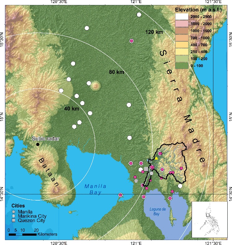
There are five rain gauges within the catchment boundaries and two river gauges along the stretch of the main channel installed since 1994 (EFCOS 2002). The rain gauges are of tipping bucket type and the river gauges are telemetry stations with an hourly digital coder that record surface water level (stage). The upstream gauging station is referred to as Montalban and drains a 380-km² upstream basin. All these gauges are maintained by the Effective Flood Control Operation System (EFCOS). Additional rain gauges within the MRB were deployed by PAGASA and NOAH in 2012.

2.2. Hydrological model

The MRB hydrological model (henceforth MRB model) was built with the modelling framework ECHSE (Kneis 2015). This software facilitates the development and deployment of object-based environmental simulation software in general and rainfall-runoff model engines in particular. As such, a model engine called HYPSO-RR (Kneis 2014a) was implemented for the MRB basin. It is a conceptual semi-distributed model that simulates the water balance dynamics within the catchment, and is mainly designed for operational applications.

The HYPSO-RR provides classes to represent run-off generation and concentration in sub-basins and streamflow in river reaches. Based on the Advanced Spaceborne Thermal Emission and Reflection Radiometer (ASTER) elevation model (a product of Ministry of Economy Trade and Industry (METI) and National Aeronautics and Space Agency (NASA)) with 30 m resolution per pixel, the MRB was discretized into sub-basins of 2.0 km² average area and reaches of 1.8 km average length using a terrain pre-processor (Kneis 2014b). Within the sub-basins, run-off generation and concentration are simulated using three conceptual flow components: surface run-off, interflow, and base flow. The external inputs include spatially variable hydro-meteorological data (rain gauge/radar-QPE, mean temperature, air pressure) and the Leaf Area Index (LAI). The LAI that represents seasonal variation is used as a proxy for crop factors in calculating for the actual evapotranspiration (ET) using the Makkink model (De Bruin 1987). A total of 15 catchment parameters are required for each sub-basin, of which 7 were independently calculated and the rest were calibrated. A detailed documentation of the model equations as well as the required input data is provided in Kneis (2015).

2.3. Streamflow and meteorological observations

The five EFCOS rain gauge stations (Mt. Oro, Nangka, Boso-Boso, Aries, and Mt. Campana) within the catchment record hourly precipitation, covering the period from 1994 to 2013, except for Mt. Campana which recorded only until 2011. Meteorological observations were interpolated to the sub-catchment centroids by inverse distance weighting. The rain gauge observations (1994–2011) were used to prepare the calibrated hydrological model. Additional rain gauges were installed by the NOAH and PAGASA starting in 2012. These new rain gauges including EFCOS were used for verification: 23 rain gauges for 2012 and 26 for 2013.

The hydrological model performance was evaluated based on the hourly discharge observed at the upstream gauge in Montalban (figure 1). Water-level data from 2004 to 2013 were subjected to a quality assurance/quality control (QA/QC) process whereby implausible values removed (e.g. sudden drops in water level or water levels that persisted over long periods). In order to convert the water level h(t) at time t to discharge Q(t), a power-law rating curve (equation 1(1) ) was developed by combining our own discharge measurements at the gauge Montalban with hydraulic considerations:(1)

The exponent n of the rating curve was obtained by hydraulic simulations using Manning's equation and the observed cross-section geometry. In order to account for potential changes in the river bed, the reference elevation h₀(t) was assumed to vary in time. For every year, h₀(t) was determined from the minimum water level at the end of the dry season, accounting for a residual flow depth of 0.5 m. The annual estimate of h₀(t) was then linearly interpolated in time. Finally, the parameter α was fitted using the discharge measurements under both base flow and flood conditions.

2.4. Model calibration

For the MRB model, calibration was carried out using an R-package for model optimization (mops) developed by Kneis (2014b). The optimization procedure is organized as a sequence of Monte Carlo (MC) simulations following the strategy of Kneis et al. (2014). The procedure starts with an MC simulation with wide, but plausible sampling ranges for all parameters. The MC ensemble consists of random parameter sets obtained by Latin Hypercube sampling. The goodness-of-fit (GOF) was computed for all ensemble members and plotted over the corresponding parameter values. Sampling ranges were then iteratively narrowed based on visual inspection of these plots until the width of the sampling ranges collapsed to zero. As GOF measures, we used per cent bias (pBias), Nash–Sutcliffe efficiency (NSE), and root-mean-square error (RMSE) expressed as follows:(2) (3) (4) where q_i is the ith out of n simulated discharge, o_i is the observation corresponding to q_i, and ω the mean of all n observations.

The model was calibrated for the period from 2004 to 2011. During that period, the model was forced by using rain gauge observations from EFCOS rain gauges. After performing the calibration, an NSE of 0.67 and a pBias of −12.5% were obtained for the entire time series of 2004–2011. Evaluating the performance of the model separately for each year reveals that only for the years 2008 and 2010, the model performs poorly – an NSE value of 0.42 and an underestimation by 23.5% for 2008 and NSE value of 0.59 and underestimation of 27.2% for 2010. The other years yield NSE value in the range 0.62–0.85 and pBias of −24% to 14.3%.

After establishing a calibrated, semi-distributed continuous hydrological model for the MRB, we evaluated different rainfall products with respect to their suitability to force the hydrological model with a specific focus on flood events.

2.5. Radar-based QPE

For radar-based rainfall retrieval, we used the open‘source radar processing library wradlib which provides functions for the most important steps in processing weather radar data for various applications (Heistermann et al. 2013b).

For radar-based rainfall estimation, we used the data from the S-band radar near Subic. The periods include wet seasons –June to October 2012, June to September 2013. Within these periods are the two Habagat events (6–9 August 2012 and 17–21 August 2013). Table 1 shows the technical specifications of the Subic S-band radar.

Table 1. Technical specifications of the Subic S-band radar.

	Subic radar
Bandwidth	S-band
Polarization	Single – Pol
Position (lat/lon)	14.822° N 120.363° E
Altitude (m a. s.l.)	532
Maximum range	120 km
Azimuth resolution	1°
Gate length	500 m
Number of elevation angles	14
Elevation angles	0.5°, 1.5°, 2.4°, 3.4°, 4.3°, 5.3°, 6.2°, 7.5°, 8.7°, 10°, 12°, 14°, 16.7°, 19.5°
Volume cycle interval	9 minutes
Data available since	March 2012

This section will provide only a brief description of the specific processing steps which mainly correspond to Heistermann et al. (2013b).

2.5.1. Clutter detection and removal

A static clutter map was established by computing the average reflectivity from four days of clear-air conditions. Based on visual inspection, radar bins exceeding a threshold of 15 dBZ were marked as a clutter. The lowest elevation angle (0.5°) was discarded because of the prohibitive clutter frequency in our study area caused by the mountain peaks of the Sierra Madre.

2.5.2. Rain rate estimation

The focus of our study is on heavy rainfall. For that reason, we used the Z(R) relation which is applied by the United States national weather service NOAA for tropical cyclones (Z = 250 ·R^1.2), where Z is the reflectivity in dBZ and R is the rainfall rate in mm/h. According to Moser et al. (2010), the use of this tropical Z(R) relation could be shown to reduce the underestimation of rainfall rates in tropical cyclones as compared to standard Z–R relationships.

2.5.3. Correcting for mean systematic bias

Subic S-band radar suffers from serious hardware miscalibration which was addressed by correcting reflectivity for the mean systematic bias. Based on a comparison with rain gauge observations in 2012 for daily temporal resolution, we detected a persistent underestimation by a factor of 4. This underestimation is assumed to be due to radar miscalibration. All measured reflectivity values from within the study period were corrected with this systematic bias.

2.5.4. Gridding and interpolation to sub-catchments

A Constant Altitude Plan Position Indicator (Pseudo-CAPPI) is generated at an altitude of 2000 m a.s.l. by using three-dimensional inverse distance weighting. The Pseudo-CAPPPI was generated from the sweeps at elevation angles of 1.5° and 2.4°. This way, we enhance the comparability of rainfall estimated at various distances from the radar. In order to use the radar data as input to the hydrological model, we interpolated the gridded data to the sub-catchments by inverse distance weighting (IDW), with a power of 2.

2.6. QPE verification using rain gauges

Conventionally, radar-based rainfall estimates are verified based on rain gauge observations. A discussion of the advantages and limitations of this approach is provided by Heistermann and Kneis (2011). We apply this strategy as one option to identify strengths and weaknesses of the radar-based rainfall estimates. Quality-controlled rain gauge observations were accumulated on hourly and daily intervals for two wet seasons: 23 rain gauges were used from June to October 2012, and 26 rain gauges from June to September 2013 (figure 1).

As quantitative verification measures, we used the pBias, NSE, and RMSE) (see Section 2.4, where q_i becomes the ith out of n precipitation estimates).

As a verification benchmark, we generated rainfall estimates by interpolating (IDW) rain gauge observations (we will refer to this as the gauge-only (GO) product). In order to evaluate the GO product, we applied a leave-one-out cross validation (LOOCV, Arlot & Celisse 2010) for each time step.

Observations of the rain gauges near and inside the MRB were specifically compared to the radar-based rainfall estimates in order to analyze potential effects on the hydrological model performance in the MRB.

2.7. QPE verification using a hydrological model

Generally, we would assume that a better rainfall product would allow for better streamflow simulations. However, different rainfall products have different error structures which imply different trade-offs. Heistermann and Kneis (2011) presented an MC approach to benchmark different precipitation products by using hydrological modelling. In our case, however, we are not so much interested in the “absolute” quality of the rainfall product. We rather want to know which rainfall product would produce better simulation of observed streamflow. On the other hand, the hydrological model was calibrated by using rain gauge observations. This implies that the calibrated model parameters might be adapted to the specific error structure of the GO product. As a consequence, a comparison between model performance based on the radar-based product and based on the GO product would be unfair. In order to efficiently overcome this problem, we re-calibrated the hydrological model for both rainfall products separately, using the procedure described in Section 2.4. We then compared the GOF measures for the corresponding re-calibrated model, based on the two wet seasons detailed in the previous section.

3. Results and discussions

3.1. Verification using rain gauges

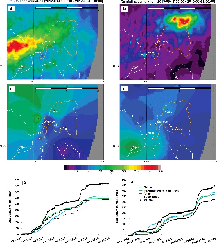
Figure 2 shows the maps of accumulated radar-based QPEs in comparison to the interpolated rain gauge observations for the two Habagat events. The MRB received extreme amounts of rainfall during both events, with the Habagat of 2012 being more serious with respect to the overall accumulated depth. For both events, the accumulated mean areal rainfall over the MRB is consistent between the radar-based QPE and the GO product. This is particularly remarkable since the underlying spatial patterns do not correspond well at all. This should be kept in mind in the following sections.

Figure 2. Comparison of the accumulated radar rainfall on the MRB (orange line) for the two Habagat events – 6–10 August 2012 (a) and 17–22 August 2013 (b) from Subic radar, and the corresponding interpolated rain gauge observations (c) and (d). The corresponding hourly accumulation graph for both radar estimates and rain gauge observations and three rain gauges within the MRB are also shown: (e) 2012 and (f) 2013. To view this figure in colour, please see the online version of the journal.

Figure 3 illustrates the estimation errors for daily rainfall accumulations during the entire verification period, for both the radar-QPE and the GO product. First, we computed the verification measures for all rain gauges in the Subic radar range (black colour). Second, we quantified those measures for a subset of rain gauges in the direct vicinity of the MRB (red colour). Table 2 provides an overview of verification results. For 2012, the radar-QPE outperforms the GO product with respect to NSE for both the entire radar range and the MRB. The radar-based QPE also shows a minimal average underestimation of only 11% for the entire radar range. For 2013, the NSE value of the radar-QPE is 0.75 and thus lower than the NSE of the GO product which is 0.82. The systematic error of the radar-QPE is also low (underestimation of 12.2% and 8.4% over the MRB). The overall NSE is very similar between radar-QPE and GO product if we focus on the MRB only (0.88 and 0.84, respectively).

Figure 3. Scatter plots for comparisons between the daily accumulations of radar-QPE (R(Z)) and rain gauge observations (GO) for all (ALL) rain gauges (black circles) and those near and inside MRB (MRB) (red circles) for 2012 and 2013. To view this figure in colour, please see the online version of the journal.

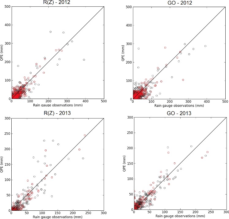
Table 2. Values of the verification measures for the daily and hourly time resolution using all available rain gauges and those near and inside the MRB.

	pBias (%)		NSE		RMSE
Evaluation period – rain gauge set	Radar	GO	Radar	GO	Radar	GO
Daily
2012 – ALL gauges	−11.2	−3.3	0.79	0.68	14.58	18.15
2012 – MRB gauges	−8.5	−5.9	0.81	0.73	12.71	15.20
2013 – ALL gauges	−12.2	6.5	0.75	0.82	17.12	14.38
2013 – MRB gauges	−8.4	13.7	0.88	0.84	13.32	15.07
Hourly
2012 – ALL gauges	−18.9	−13.9	0.45	0.18	4.29	5.24
2012 – MRB gauges	−16.2	−13.7	0.32	0.01	7.21	8.71
2013 – ALL gauges	−13.9	11.4	0.25	0.29	4.28	3.57
2013 – MRB gauges	−7.8	4.8	0.40	0.41	3.84	3.80

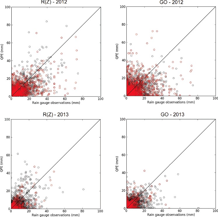
The hourly verification (figure 4 and table 2) shows much more scatter than the daily verification. This is primarily due to a lower representativeness of the point measurement at this temporal scale. The relative performance of the radar-QPE as compared to the GO product is consistent, though, with the daily verification. As we use hourly data for running the hydrological model, it will be interesting to see whether the apparently huge random error of the rainfall estimation at this time scale also translates to the simulated streamflow for a meso-scale basin such as the MRB, or whether these random errors are sufficiently smoothed in space and time by the integrated hydrological response of the catchment.

Figure 4. The same as figure 3 but for hourly accumulations. To view this figure in colour, please see the online version of the journal.

3.2. Verification using the hydrological model

From June to October 2012 and June to September 2013, we used both the radar-based QPE as well as the GO product to force the hydrological model of the MRB. These periods represent a coherent radar data-set and captured two remarkable floods as well as a couple of moderate events. For a fair comparison of these two rainfall products, we re-calibrated the hydrological model separately for each of the rainfall input data-sets (see Section 2.7). At the beginning of the two verification periods, the model was initialized with the state variables obtained from previous simulations using the spatially interpolated rain gauge observations from EFCOS.

As shown in figures 5 and 6, the model driven by hourly radar-based QPEs yields a simulated streamflow that corresponds well with both the major peaks (associated with the Habagat events mentioned earlier) and the low flows – despite the poor hourly verification results illustrated by figure 4. As already hypothesized in Section 3.1, the hydrological catchment response appears to smooth and compensate random errors contained in the rainfall input. The NSE achieved by the model driven by radar-QPE ranges between 0.72 and 0.85. This range includes both the contiguous wet seasons and the two Habagat-induced flood events.

Figure 5. Observed and simulated hourly streamflow using rain gauge observations and radar rainfall for the period 10 June to 14 October 2012 (upper), and 7 June to 9 September 2013 (lower) and the corresponding rainfall estimates from rain gauges and radar. Black rectangles mark the floods during the Habagat events. Values of the goodness-of-fit measures were also indicated for each year.

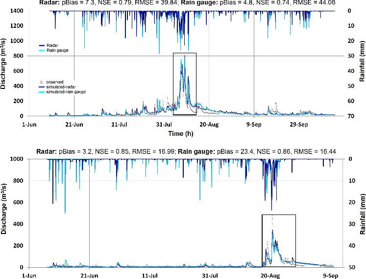
Figure 6. Hydrographs of the floods brought by the Habagat events (marked with black rectangles in the figure 5) for the years 2012 (upper) and 2013 (lower). Values of the goodness-of-fit measures were also indicated for each year.

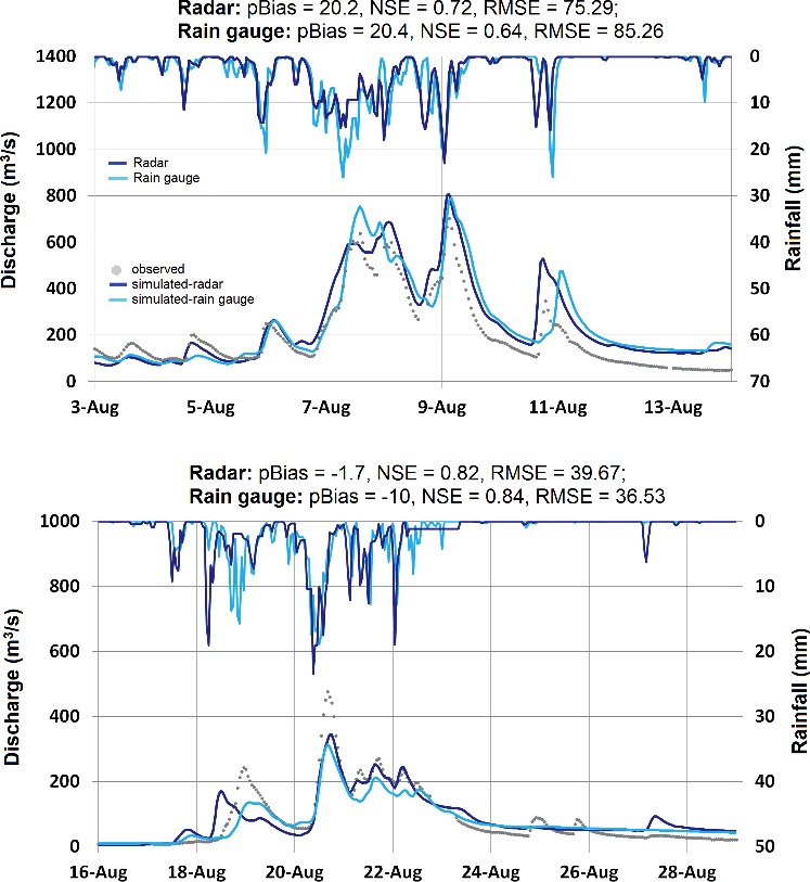
The model driven by the GO product also performs comparably well in terms of NSE (between 0.64 and 0.86), but exhibits a larger bias (−10.0% to 23.4%). It is clearly outperformed by the radar-QPE in 2012 and almost equivalent in 2013.

In general, the radar-QPE driven model yields a better representation of the observed major streamflow peaks and hydrograph shape than the rain gauge driven model. Smaller peaks, however, are mostly underestimated by the model driven by the radar-based QPE, while overestimated by the model using the GO product.

Table 3 summarizes the performance of the radar-based QPE and GO QPE in streamflow simulations for the 2012 and 2013 wet seasons, and the corresponding major flood events (Habagat events).

Table 3. Summary of the performance of hydrological simulations using the two QPEs for different evaluation periods.

	pBias (%)		NSE		RMSE
Evaluation period	Radar	GO	Radar	GO	Radar	GO
2012 (Jun–Oct)	7.3	4.8	0.79	0.74	39.84	44.06
2013(Jun–Sep)	3.2	23.4	0.85	0.86	16.99	16.44
Habagat-induced flood 2012	20.2	20.4	0.72	0.64	75.29	85.26
Habagat-induced flood 2013	−1.7	−10.0	0.82	0.84	39.67	36.53

On this basis, we can compare the results of the hydrological verification with the results of the point-based verification (previous section). Both verification approaches are consistent in several respects: for both verification approaches, the radar-based QPE is superior to the GO QPE in 2012 and almost equivalent to the GO QPE in 2013. Discrepancies in the performance of the QPE methods as identified by the point-based verification shrink in the hydrological verification. This is plausible. First, the recalibration of the model using the “competing” rainfall estimates can reduce the effects of estimation errors on simulated streamflow. This particularly applies to systematic error components. Second, as already mentioned, the random rainfall estimation errors are smoothed out in both space and time by the hydrological catchment response. These mechanisms might have been effective particularly in 2013 in levelling out the differences between the radar-based QPE and the GO QPE. Recalling the striking differences in the spatial rainfall patterns as shown in figure 2, it appears surprising that, in 2013, the model driven by the GO QPE can compete with the model driven by the radar-based QPE. Moreover, while the rain gauges seem to fail entirely in representing the spatial rainfall distribution over the catchment, both rainfall estimation methods are more or less consistent with regard to the mean areal rainfall (figure 2). The spatial filter effect of the hydrological model together with the recalibration might be the reason that the model driven by the GO QPE still shows a moderate performance. At the same time, the GO QPE also achieved good verification results in the LOOCV, presumably because the rain gauges close to each other observed similar rainfall depths. However, it would require longer time series in order to evaluate whether the verification results of the GO QPE in 2013 are dominated by random effects.

4. Conclusions

In this case study, we evaluated the potential of radar-based rainfall estimates to force a continuous, semi-distributed hydrological model of the MRB in the Philippines. As a benchmark, we used rainfall estimates purely based on interpolated rain gauge observations (GO product). The analysis is based on data from the wet seasons of the years 2012 and 2013. We evaluated the rainfall products with respect to their ability (1(1) ) to represent rainfall at the point scale (i.e. to reproduce rain gauge observations), and (2(2) ) to reproduce observed streamflow (catchment scale).

Both verification approaches are consistent with regard to their main results: for the 2012 wet season and the corresponding major flood event, the radar-based QPE is clearly superior to the gauge-based QPE. In 2013, both rainfall estimation methods show a similar performance. As for the point-based verification, the daily verification results indicated a much better correlation with the reference rainfall than the hourly verification, supposedly due to representativeness issues. Despite the poor hourly verification results at the point scale, both rainfall estimates produced a good representation of hourly streamflow when used as input to the hydrological model. Particularly in 2013, it was surprising that the hydrological verification of both rainfall products yielded more or less equivalent results, although the rain gauges seemed to fail entirely in representing the spatial rainfall distribution of the major rainfall event. However, future research has to show whether this is rather a random effect.

Since the MRB is, for Philippine conditions, quite densely monitored by rain gauges, the verification results are particularly promising towards the use of radar-based rainfall estimates for hydrological simulations and forecasting in other parts of the country where rain gauge density is even lower. The potential of the radar-based rainfall estimation might as well be underestimated in this study since the serious radar miscalibration decreases the signal-to-noise ratios. Thus, we suggest addressing this issue as a priority in radar maintenance. In terms of transferability, we would like to emphasize though, that the quality of the radar-based rainfall estimation varies in space, and of course also depends on the radar device. The same applies to the hydrological modelling approach which still has to be verified for other parts of the Philippines.

Hence, the highest priority for future research is to investigate the transferability of the presented methods to other catchments and radars in the Philippines, and to evaluate the added value of radar-based rainfall estimates for short-term stream forecasting, in combination with rainfall forecasts.

Acknowledgements

We would like to thank the Philippine Atmospheric, Geophysical and Astronomical Services Administration (PAGASA) for generously providing the radar data. The NOAH (National Operational Assessment of Hazards) project and the EFCOS (Effective Flood Control Operation and Services) provided the rain and river gauge data. This study is funded by Helmholtz Association through the GeoSim Graduate Research School. We also thank Bernard Allan Racoma, Justine Perry Domingo, Pamela Tolentino, Mark Clutario, Joan de Vera, Gerald Quiña, and Carlo Manalansan for assisting in the field works. We would like to thank two anonymous referees for helpful comments on a previous version of this manuscript.

Disclosure statement

No potential conflict of interest was reported by the authors.

Additional information

Funding

GeoSim Graduate Research School: Helmholtz Association

References

- Abon CC, David CPC, Pellejera NEB. 2011. Reconstructing the tropical storm Ketsana flood event in Marikina River, Philippines. Hydrol Earth Syst Sci. 15:1283–1289.
- Arlot S, Celisse A. 2010. A survey of cross-validation procedures for model selection. Stat Surv. 4:40–79.
- Atencia A, Mediero L, Llasat MC, Garrote L. 2011. Effect of radar rainfall time resolution on the predictive capability of distributed hydrologic model. Hydrol Earth Syst Sci. 15:3809–3827.
- Berne A, Krajewski WF. 2013. Radar for hydrology: Unfulfilled promise or unrecognized potential? Adv Water Res. 51:357–366.
- Borga M. 2002. Accuracy of radar rainfall estimates for streamflow simulation. J Hydrol. 267: 26–39.
- De Bruin HAR. 1987. From Penman to Makkink In: Hooghart JC, editor. Evaporation and weather. Proceedings and information No. 39. The Hague: TNO Committee on Hydrological Research; 1191 p.
- [DPWH] Department of Public Works and Highways. 2004. Water and floods: a look at Philippine rivers and flood mitigation efforts. Manila: DPWH.
- [EFCOS] Effective Flood Control Operation System. 2002. CTI International Engineering report on technical guidance for the project for rehabilitation of the flood control operation and warning system in Metro Manila. Manila: EFCOS.
- Germann U, Berenguer M, Sempre-Torres D, Zappa M. 2009. REAL – ensemble radar precipitation estimation for hydrology in mountainous region. Q J R Meteorol Soc. 135:445–456.
- Heistermann M, Crisologo I, Abon CC, Racoma BA, Jacobi S, Servando NT, David CPC, Bronstert A. 2013a. Brief communication: Using the new Philippine radar network to reconstruct the “Habagat of August 2012” monsoon event around Metropolitan Manila. Nat Hazards Earth Syst Sci. 13:653–657.
- Heistermann M, Jacobi S, Pfaff T. 2013b. Technical note: an open source library for processing weather radar data (wradlib). Hydrol Earth Syst Sci. 17:863–871.
- Heistermann M, Kneis D. 2011. Benchmarking quantitative precipitation estimation by conceptual rainfall-runoff modeling. Water Resour Res. 47:W06514 doi:10.1029/2010WR009153
- Kneis D. 2014a. Eco-Hydrological Simulation Environment (ECHSE): documentation of model engines. Potsdam: Institute of Earth and Environmental Sciences, University of Potsdam.
- Kneis D. 2014b. Eco-Hydrological Simulation Environment (ECHSE): documentation of pre- and post-processors. Potsdam: Institute of Earth and Environmental Sciences, University of Potsdam.
- Kneis D. 2015. A lightweight framework for rapid development of object-based hydrological model engines. Environ Model Softw. 68:110–121.
- Kneis D, Chatterjee C, Singh R. 2014. Evaluation of TRMM rainfall estimates over a large Indian river basin (Mahanadi). Hydrol Earth Syst Sci. 18:2493–2502.
- Liongson LQ. 2008. Flood mitigation in Metro Manila. Philipp Eng J. 29:51–66.
- Moser H, Howard K, Zhang J, Vasiloff S. 2010. Improving QPE for tropical systems with environmental moisture fields and vertical profiles of reflectivity. In: Extended abstracts for the 24th Conference on Hydrology. American Meteorological Society. Available from: https://ams.confex.com/ams/pdfpapers/162510.pdf
- [NDRRMC] National Disaster Risk Reduction and Management Council. 2013. Site rep no. 20 re effects of Southwest monsoon (HABAGAT) enhanced by tropical storm “Maring.” Manila: NDRRMC.
- [PAGASA] Philippine Atmospheric Geophysical and Seismological Administration. 2004. Climate map of the Philippines based on modified Coronas classification. Available from: http://kidlat.pagasa.dost.gov.ph/index.php/climate/climate-monitoring
- Sauvageot H. 1994. Rainfall measurement by radar: a review. Atmos Res. 35:27–54.
- Sun X, Mein RG, Keenan TD, Elliott JF. 2000. Flood estimation using radar and rain gauge data. J Hydrol. 239:4–18.
- Terblanche DE, Pegram GGS, Mittermaier MP. 2001. The development of weather radar as a research and operational tool for hydrology in South Africa. J Hydrol. 241:3–25.
- Villarini G, Smith JA, Baeck ML, Sturdevant-Rees P, Krajewski WF. 2010. Radar analyses of extreme rainfall and flooding in urban drainage basins. J Hydrol. 381:226–286.
- Yang D, Koike T, Tanizawa H. 2004. Application of a distributed hydrological model and weather radar observations for flood management in the upper Tone River of Japan. Hydrol Process. 18:3119–3132.