Mapping earthquake-triggered landslide susceptibility by use of artificial neural network (ANN) models: an example of the 2013 Minxian (China) Mw 5.9 event

Abstract

A landslide susceptibility map, which describes the quantitative relationship between known landslides and control factors, is essential to link the theoretical prediction with practical disaster reduction measures. In this work, the artificial neural network (ANN) model, a promising tool for mapping landslide susceptibility, was adopted to evaluate the coseismic landslide susceptibility affected by the 2013 Minxian, Gansu, China, Mw5.9 earthquake. The evaluation was based on the landslide inventory of this event containing 6479 landslides, and the terrain, geological and seismic factors from database available. During the analyses, two ANN models were applied: considering the entire factors aforementioned (CS model) and excluding seismic factors above (ES model). The success and predictive rates of ANN models and the cumulative percentage curves of susceptibility maps obtained from the models all indicate that the CS model has a relatively better performance than the ES model. However, the comparison of overlapping susceptibility areas suggests that 52.8% of the very high susceptibility areas derived from the CS model coincide with the ES model; and for the very low susceptibility areas, this proportion is 73.55%. Thus, it can be concluded that the assessment based on existing earthquake-induced landslides and the ES model could provide better background information for seismic landslide susceptibility mapping and disaster prevention.

Keywords:

• Seismic landslides
• Minxian earthquake
• artificial neural network
• susceptibility assessment
• seismic factors

1. Introduction

Earthquake-induced landslides are one of the main natural hazards which seriously threaten the life and property of human beings. For instance, there were about 200,000 landslides caused by the 2008 Wenchuan, China Mw 7.9 earthquake, which occupied a total area of 1160 km² with a total volume larger than 10 billion m³, resulting in huge casualties and hundreds of billions RMB economic losses (Yin et al. 2009; Xu et al. 2014b; Xu et al. 2016b). Another recent example is the 2015 Gorkha, Nepal Mw 7.8 earthquake, which triggered more than 2064 landslides with an area larger than 10 thousand m², covering a total area of 44.78 km² with the estimated average volume of 509 million m³ (Xu et al. 2016c).

Most research related to the earthquake-induced landslides is based on the coseismic landslide inventory. So far, many coseismic landslide inventories have been published, which were used to delineate the spatial distribution of landslides, prepare susceptibility maps, study the impact of slope failure on landscape evolution, and invert seismogenic mechanism (Keefer 2000; Kamp et al. 2010; Parker et al. 2011; Gorum et al. 2013; Xu et al. 2015a, 2017; Rao et al. 2017). Only by making clear the mechanisms of past landslide hazards, can they be prevented and mitigated effectively when future earthquakes strike the same area once again (Guzzetti et al. 2006). However, it is difficult to identify the mechanism of every landslide in a large area. From a regional perspective, it is the susceptibility assessment that is generally accepted as a final product to link the theoretical analyses with practical disaster reduction measures (Hong et al. 2016b). The preparation of seismic landslide susceptibility maps commonly uses the methods in research on rainfall-induced landslides for reference. Integrating the evaluation model and the relationships between landslide data and the related control factors permits to determine the landslide-prone conditions and help prevent and mitigate the disaster (Lee et al. 2007; Tien Bui et al. 2012b). Thus, to a given area, the selection of evaluation models and control factors decide the accuracy of a landslide susceptibility map. The commonly used models include logistic regression, certainty factor, information value, weight of evidence, and so on (Xu et al. 2013a; Bai et al. 2014; Dou et al. 2015a; Chen et al. 2017b; Tian et al. 2017a). For example, Xu et al. (2012b) delineated the landslide-prone areas in the Qingshui River watershed of the 2008 Wenchuan earthquake struck region by using thirteen controlling factors, landslide data and the weight of evidence model. Though many methods and technologies can be used to map the landslide susceptibility, there is still no agreement on the optimal model (Wang et al. 2005; Yesilnacar and Topal 2005; Regmi et al. 2013). With the development of machine learning technologies, lots of unconventional statistical methods have been proposed to map the landslide susceptibility, such as the artificial neural network (ANN), decision tree, and support vector machine (Tien Bui et al. 2013, 2017; Hong et al. 2016a, 2017b). For example, using the support vector machine model, eighteen control factors and the landslide data in the study area, Lee et al. (2017) mapped the landslide susceptibility for the Pyeong Chang and Inje areas of Gangwon Province, Korea. Nowadays, lots of aforementioned methods have been applied to mapping earthquake-induced landslide susceptibility (Xu et al. 2012a; Wang et al. 2016; Chen et al. 2017a). Among them, the ANN model shows a good performance for classification and prediction (Pradhan and Lee 2009; Yilmaz 2009a, 2010; Dou et al. 2015b; Lee et al. 2016). For example, Pradhan and Lee (2010) assessed the landslide susceptibility using a back-propagation (BP) artificial network model for the Klang Valley. Their results suggest that the ANN model has a better performance with the predictive accuracy of 94%. The second disagreement is the number of the control factors which are used to train the evaluation model (Tien Bui et al. 2011; Hong et al. 2017a). When mapping the landslide susceptibility in the Klang Valley area, Malaysia, Pradhan and Lee (2010) analyzed three cases about the factor selection in their study: 11 factors, 7 factors (removal of 4 factors with smallest weights), and 4 factors (removal of the remaining three factors with least weights). The results show that the case with seven factors has the best accuracy. Therefore, the selection of the control factors plays an important role in landslide susceptibility mapping.

After the 2013 Minxian, China Mw5.9 earthquake, only a little research was published concerning the landslides triggered by this event. However, Minxian is an earthquake-prone area, and apparently its terrain and geological conditions imply a high probability of landsliding. Moreover, this region belongs to a part of the Belt and Road Initiative. Therefore, mapping the landslide susceptibility is very important in this region. In this study, the affected area of the 2013 Minxian Mw 5.9 earthquake was taken as an example for mapping landslide susceptibility by use of the ANN model. Ten control factors (elevation, slope angle, slope aspect, curvature, slope position, distance to drainages, lithology, earthquake intensity, peak ground acceleration, and distance to the seismogenic fault) were considered. For the purpose of disaster prevention and mitigation in the seismically active area, the cases considering (CS) and excluding (ES) seismic factors were compared in this study. The software platforms used in this study include ArcGIS 10.4, Weka 3.7 and Matlab R2014a.

2. Tectonic setting and study area

Due to the effect of the India-Eurasia plate collision, the northeastern margin of the Tibetan Plateau hosts very active tectonics (Figure 1(a)). A great deal of large-scale active faults developed there. Among them, the West Qinling fault (F1) and East Kunlun fault (F3) are the two large-scale strike-slip structures. Their relative movements generate a rock bridge area in which there are a series of thrust faults with left slip components (Figure 1(b)). The Lintan–Dangchang fault (F2) is one of these thrust faults, which has several branches. On 22 July 2013, one branch (F2-2 in Figure 1(c)) of the Lintan–Dangchang fault was ruptured by the Minxian Mw 5.9 earthquake (He et al. 2013) with the epicenter nearby the bending of the Tao River and the focal depth about 20 km.

Figure 1. (a) Regional location of study area. (b) Major faults and the limit of coseismic landslides of the 2013 Minxian earthquake (grey ellipse). F1: West Qinling fault; F2: Lintan–Dangchang fault, F2-1, F2-2, F2-3, and F2-4 are its branches; F3: East Kunlun fault. (c) Distributions of faults and coseismic landslides in the study area. Source: Author.

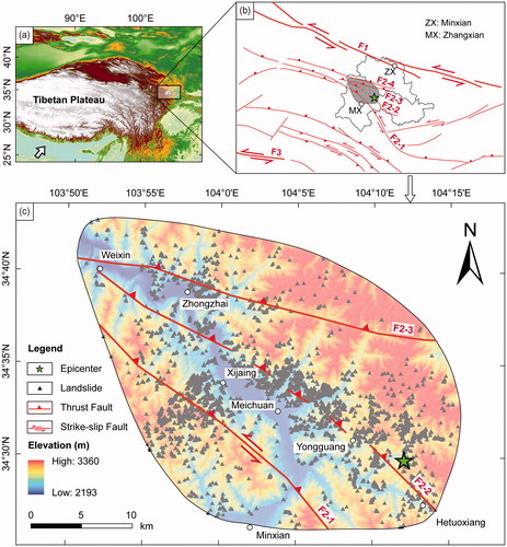
Despite its moderate magnitude, the 2013 Minxian earthquake has triggered a large number of coseismic landslides. Statistics show that the earthquake and its secondary effects led to several billion RMB of economic losses and affected hundreds of thousands of people (Tian et al. 2016). Combined with the results of field investigation and comparative analyses of remote sensing images collected close to the origin time, the approximate area affected by coseismic landslides of 873.95 km² was delineated as the study area. The elevation of this area ranges from 2193 m to 3360 m with an average of 2695 m, and the east side of Tao River is much higher than the west side. The slope angles range from 10° to 80.7° with an average of 24°. The earthquake struck area belongs to transition regions of temperate semi-humid to high and cold humid climate. The annual average precipitation is about 600 mm. The one-week accumulative antecedent precipitations are about 10–20 mm in the study area before the earthquake (Tian et al. 2017b).

3. Data and methods

3.1. Coseismic landslides caused by the 2013 Minxian Earthquake

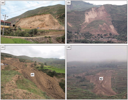
Following the principles of preparing earthquake-triggered landslide inventories (Xu 2015), a detailed landslide inventory for the 2013 Minxian event has been constructed. It was based on field investigations and the remote sensing images before and after the event. According to the differences of colors, textures and terrains between the pre- and post-earthquake images, coseismic landslides triggered by the 2013 Minxian earthquake were mapped. Consequently, a polygon database including 6479 coseismic landslides was created (Tian et al. 2016) (Figure 1(c)). These landslides occupy about 1.76 km², nearly 50% of which are smaller than 100 m², and only less than 10% exceed 500 m². The majority of these landslides are distributed along the loess scarps, dominated by soil slides and flows (Figure 2).

Figure 2. Photos showing typical landslides in the study area: (a) landslide in Chuanducun, (b) landslide in Weixincun, (c) Yongguangcun 1# landslide, and (d) Yongguangcun 2# landslide.

3.2. Control factors

The quantity and accuracy of control factors determine the quality of landslide susceptibility maps (Tien Bui et al. 2016). In spite of no unanimous selection standards for control factors (Xu et al. 2013b), it is commonly accepted that the factors concerning terrain, geology, and seismology are most significant for spatial susceptibility assessment of earthquake-induced landslides (Dai et al. 2011; Xu et al. 2013c, 2015b). Ten control factors were considered in this study, namely six terrain factors (elevation, slope angle, slope aspect, curvature, slope position, and distance to drainages), one geological factor (lithology), and three seismic factors (earthquake intensity, peak ground acceleration, and distance to the seismogenic fault). In order to obtain a high-quality susceptibility map, 5-m-resolution ALOS DEM was used to extract the terrain factors in this study. The geological and seismic factors were derived from websites of NGAC (National Geological Archives of China, http://geodata.ngac.cn/), CEA (China Earthquake Administration, http://www.cea.gov.cn), and USGS (United States Geological Survey, https://earthquake.usgs.gov). The specific descriptions of these control factors are as follows.

3.2.1. Elevation

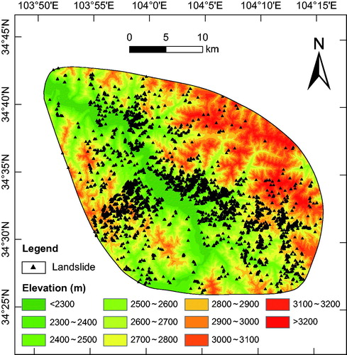
Elevation has a complicated relationship with the distribution of earthquake-triggered landslides. The mass at a higher slope altitude would become unstable when it suffers large topography magnification from seismic waves. However, slope material at a lower elevation nearby rivers can also be subject to landsliding. No matter what kind of effect it would be, elevation does have a major control on landslides. The elevation range of the study area was categorized into 11 sets with a100-m interval (Figure 3): (1) < 2300 m; (2) 2300–2400 m; (3) 2400–2500 m; (4) 2500–2600 m; (5) 2600–2700 m; (6) 2700–2800 m; (7) 2800–2900 m; (8) 2900–3000 m; (9) 3000–3100 m; (10) 3100–3200 m; and (11) > 3200 m.

Figure 3. Classifications of elevation in the study area.

3.2.2. Slope angle

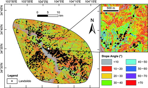
Slope angle describes the inclination of the slope surface. It can be defined by the maximum rate of elevation differences between one cell and its neighbours. The homogeneous and steeper slopes have larger gravity components to slide along the slope surface, thus slopes with larger slope angles are more prone to slide (Xu and Xu 2013). Using a ten-degree interval, the slope angle in the study area is divided into eight classes: (1) < 10$°$; (2) 10$°$–20$°$; (3) 20$°$–30$°$; (4) 30$°$–40$°$; (5) 40$°$–50$°$; (6) 50$°$–60$°$; (7) 60$°$–70$°$; and (8) > 70$°$ (Figure 4).

Figure 4. Classifications of slope angle in the study area.

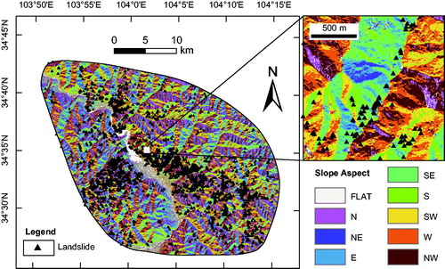
3.2.3. Slope aspect

Slope aspect refers to the facing direction of a slope surface. Different slope aspects may be subject to varied effects of light, temperature, rainfall, and wind. This would in turn influence the type and distribution of vegetation and the weathering of slope materials (Dai and Lee 2002). Furthermore, the higher weathering materials are easier to slide. In this study, the acknowledged aspect classifications were employed as follows: (1) FLAT (–1); (2) N (North, 0$°$–22.5$°$ and 337.5$°$–360$°$); (3) NE (Northeast, 22.5$°$–67.5$°$); (4) E (East, 67.5$°$–112.5$°$); (5) SE (Southeast, 112.5$°$–157.5$°$); (6) S (South, 157.5$°$–202.5$°$); (7) SW (Southwest, 202.5$°$–247.5$°$); (8) W (West, 247.5$°$–292.5$°$); and (9) NW (Northwest, 292.5$°$–337.5$°$) (Figure 5).

Figure 5. Classifications of slope aspect in the study area.

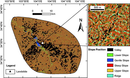
3.2.4. Slope position

Slope position is a scale-based parameter which characterizes the relative slope positions in a given region (Weiss 2001). It is qualified by the topographic position index (TPI) and slope angle. According to Jenness et al. (2013), the six categories of slope positions are (1) valley with extreme low TPI value; (2) lower slope with moderately low TPI value; (3) gentle slope with TPI value around 0 and slope angle $\le$ 5$°$; (4) steep slope with TPI value around 0 and slope angle $>$ 5$°$; (5) upper slope with moderately high TPI value; and (6) ridge with extreme high TPI value. The classification of slope positions in the study area is shown in Figure 6.

Figure 6. Classifications of slope position in the study area.

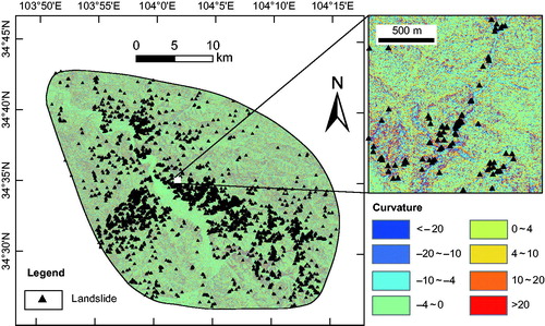
3.2.5. Curvature

Curvature refers to the bending of a slope plane. A positive curvature means the slope surface is convex outwards. By contrast, a negative curvature indicates the slope surface is concave inwards. Moreover, the zero value is to say that the slope surface is close to straight and flat. Generally speaking, the convex and concave slopes are more prone to sliding than flat slopes (Xu et al. 2014a). The factor of curvature includes eight categories according to the classification results (Figure 7): (1) < –20; (2) –20 to –10; (3) –10 to –4; (4) –4 to 0; (5) 0–4; (6) 4–10; (7) 10–20; and (8) > 20.

Figure 7. Classifications of curvature in the study area.

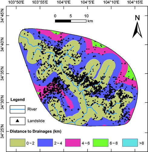
3.2.6. Distance to drainages

The landforms of free surfaces due to erosion and excavation near rivers provide favourable conditions for landslide occurrence. Therefore, landslides are often distributed along drainages. In this study, the buffers were created around the rivers with larger accumulation to study the relationships between landslides and distance to drainages. The study area was classified into 5 classes with a buffered distance interval of 2 km: (1) 0–2 km; (2) 2–4 km; (3) 4–6 km; (4) 6–8 km; and (5) > 8 km (Figure 8).

Figure 8. Classifications of distances to drainages in the study area.

3.2.7. Lithology

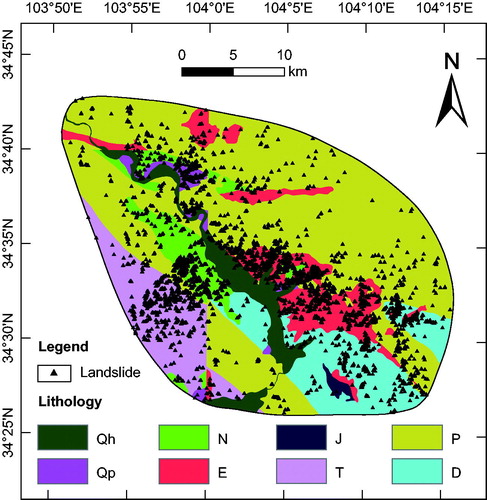
Lithology, which characterizes the slope-forming material, affects the properties of slopes, such as the slope strength and permeability (Dai and Lee 2002). Therefore, it is an important factor affecting the landslide distribution. The strata of eight stratigraphic ages with different lithology are distributed in the study area, namely (1) Holocene (Qh): Sand and gravel; (2) Late Pleistocene (Qp): Sand, gravel beds, and sand loess; (3) Neogene (N): Sandstone, conglomerate, claystone, and sandy mudstone; (4) Eogene (E): Sandstone, conglomerate; (5) Jurassic (J): Conglomerate, carbonaceous shale clip coal, or oil shale; (6) Triassic (T): Thick sandstone, slate, and a small amount of limestone; (7) Permian (P): carbon-containing slate, slate, sandstone, conglomerate; (8) Devonian (D): silty slate, powder sandstone, slate. The strata with varied lithology above in the study area are depicted in Figure 9.

Figure 9. Strata-based classifications of lithology in the study area (see text).

3.2.8. Peak ground acceleration (PGA)

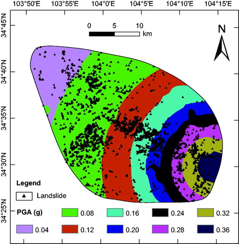
PGA is the maximum change of ground shaking velocity recorded by seismometers during an earthquake. It is a measure of how strong the ground shakes at a given site. The intense shakes can trigger slope failure. The PGA data downloaded from the USGS website (https://earthquake.usgs.gov/earthquakes/eventpage/usb000ije3#shakemap) indicate that there are nine levels of PGA in the study area: (1) 0.04 g; (2) 0.08 g; (3) 0.12 g; (4) 0.16 g; (5) 0.20 g; (6) 0.24 g; (7) 0.28 g; (8) 0.32 g; and (9) 0.36 g (Figure 10).

Figure 10. Classifications of PGA in the study area.

3.9.10. Earthquake intensity

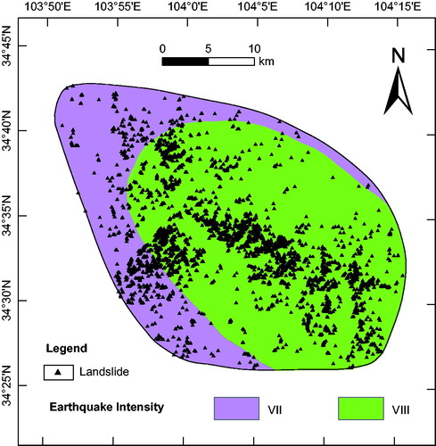
Earthquake intensity, published by the China Earthquake Administration, is an index to express how strong the ground shaking and its impact resulted from an earthquake are. It is estimated by the human feelings, building damages, other damages and horizontal motion on the ground and classified into twelve degrees in Roman numerals from I (insensible) to XII (landscape reshaping) (The Chinese seismic intensity scale (GB/T 17742-2008); https://en.wikipedia.org/wiki/China_seismic_intensity_scale). Usually, more landslides may occur on slopes in the higher seismic intensity area. Relevant data have established that the study area of this work is located in the regions of VII- and VIII-intensity (Figure 11).

Figure 11. Classifications of earthquake intensity in the study area.

3.9.11. Distance to the seismogenic fault

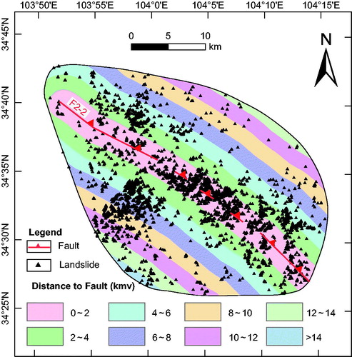
The landslides triggered by earthquakes are usually distributed linearly along the seismogenic fault (Kamp et al. 2008; Gorum et al. 2011; Lee 2014; Xu and Xu 2014). In general, with the increasing distance away from the causative fault, the quantity and scale of landslides would obviously decrease. Eight portions were sliced based on the distances to the seismogenic fault (F2-2) in the study area, namely (1) 0–2 km; (2) 2–4 km; (3) 4–6 km; (4) 6–8 km; (5) 8–10 km; (6) 10–12 km; (7) 12–14 km; and (8) > 14 km (Figure 12).

Figure 12. Classifications of distance to the seismogenic fault in the study area.

3.3. Artificial neural network model

Given that the limitations of statistical techniques of oversimplification, prohibitive data requirements and ineffective input data acquisition, an alternative machine learning technology named ANN is adopted in this work, This method imitates the neural network of human brains to apply the experience learned via samples to recognize new unseen data, gradually mature through several decades (Gómez and Kavzoglu 2005; Yilmaz 2009b). ANN is characterized by the features of the independent statistical distribution of the data, self-learning, and associative memory. It has a remarkable ability for handling imperfect or incomplete data and the nonlinear and complex problems. Therefore, though it is not known exactly how it works (known as a black box), the ANN model has widely been used in pattern recognition, classification, regression, autocorrelation, prediction, and other fields.

The BP neural network is one of the most commonly used ANN learning algorithms and was applied in this study. It consists of input, hidden and output layers. The input and output layers are to ANN what the dendrite and axon are to the neurons of the human brain, respectively. There are many neurons in the model which are connected in layers. During the course of learning, the input signals travel from the input layer through the hidden layer to the output layer by multiplying corresponding weights. Next, the resulting signals are summed up and processed by the transfer function to obtain the outputs. Then the errors between the actual and target outputs are calculated and back propagated starting at the output layer to adjust the corresponding weights till the threshold conditions are satisfied, and this is how the ANN model learns. Finally, an optimized model can be built to validate testing data or apply in other similar conditions. The sigmoid function is a transfer function commonly employed in ANN to introduce nonlinearity transformation. It is defined by formula f(x) = 1/(1 + e^(–x)) and produces an “S” shape curve (Lee et al. 2003, 2004; Gómez and Kavzoglu 2005).

The ANN model is a useful tool in assessing the probability of landslides, which can be used to forecast the future landslides according to the distribution of past ones (Yilmaz 2009b). The landslide susceptibility assessment can be regarded as a binary classification (landslide and non-landslide), and what we want to do is to identify the areas of landslide and non-landslide (Hong et al. 2015a). To control the over-fitting of the model, the landslide samples were split into two parts separately to train and test the model (Ripley 1996; Tien Bui et al. 2012a). The total 6479 landslides induced by the 2013 Minxian earthquake were divided into two sets: training landslide dataset (4536, accounting for 70%) and testing landslide dataset (1943, accounting for 30%). The equivalent points of training and testing datasets of non-landslide were randomly selected outside the 5 m buffers of these coseismic landslide polygons to minimize the influence from the landslides. Consequently, 9072 points and 3886 points with extracted information of control factors were applied to train and test the ANN model, respectively.

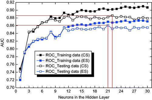
The aforementioned control factors were imported into the model corresponding to the nodes of the input layer. The classification results of landslide and non-landslide were assigned to two sets of nodes in the output layer. The parameters of learning rate and momentum were set as defaults 0.3 and 0.2, respectively. The number of epochs was 500 by default. The accuracy of the ANN model could be improved by changing the number of neurons in the hidden layer. According to Tien Bui et al. (2016), by comparing the areas under curves (AUC for short) of the ROC (receiver operator characteristics) of training data and testing data in varying numbers of neurons, the optimal number of the nodes in the hidden layer can be determined.

For the sake of promoting the ability to prevent and reduce landslide disaster before future earthquakes, two cases were considered in the ANN analysis: one uses all the control factors aforementioned, and the other uses those but excluding the seismic factors. The case considering the seismic factors is marked by CS, and another excluding these factors is marked by ES.

4. Results

4.1. Architectures of the ANN models

The AUCs of training data and testing data versus the numbers of neurons in the hidden layer are shown in Figure 13. With the increasing number of the neurons, the indexes above both increase firstly and then fluctuate in a certain range. The results indicate that the AUCs of predictive ratio curves for testing data are the largest when there are 22 and 21 nodes in the hidden layers of CS and ES models, respectively.

Figure 13. The number of neurons in the hidden layer versus AUC concerning training data and testing data. CS: the case of considering seismic factors (earthquake intensity, PGA, and distance to the seismogenic fault); ES: the case of excluding seismic factors (the same hereinafter).

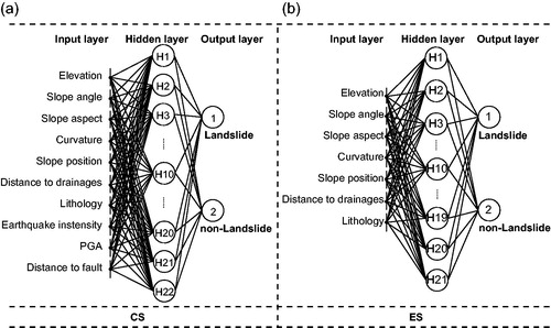
Based on the Minxian coseismic landslides and control factors, the CS and ES models were built. The architectures of the ANN models are shown in Figure 14.

Figure 14. Architectures of the ANN models: (a) CS model and (b) ES model.

4.2. Performances of the ANN models

Using the above landslide data along with the ANN models, the relevant assessment indexes of the training and testing results were calculated (Table 1). Sensitivity and specificity were used to measure the performances of classification tests. As shown in Table 1, for the CS model, the sensitivity and specificity of the training data are 81.43% and 85.19%, respectively; for the testing data, they are 80.74% and 82.56%, respectively. It means that there are 81.43% and 80.74% of the total landslide samples in the training and testing data were correctly classified, respectively; and 85.19% and 82.56% of the non-landslide samples were correctly classified, respectively. The classification accuracy of the training process is 83.20%; and for testing process is 81.63%. As for the ES model, the sensitivity and specificity of the training data are 75.50% and 82.17%, respectively; for the testing data, they are 75.19% and 80.87%, respectively. It means that there are 75.50% and 75.19% of the landslide samples in the training and testing data were correctly classified, respectively; and 82.17% and 80.87% of the non-landslide samples were correctly classified, respectively. The classification accuracy of the training process is 78.45%; and for testing process is 77.74%. However, the Kappa values of the training and testing data for the CS model are 0.66 and 0.63; and for the ES model, they are 0.569 and 0.55. The Kappa value represents the agreement between processed results and the reality. When it exceeds 0.61, it means a substantial agreement. The ES model with lower Kappa values shows a moderate agreement between the processed results and the realistic landslide distribution. Because of the error of sampling methods for the landslide and non-landslide points, the ANN models could also be accepted to map the landslide susceptibility in the whole study area.

Table 1. Performances of the ANN models.

No.	Index	CS model		ES model
		Training data	Testing data	Training data	Testing data
1	Correctly classified instances	7548	3172	7117	3021
2	Incorrectly classified instances	1524	714	1955	865
3	True positive (TP)	3902	1614	3821	1609
4	True negatives (TN)	3646	1558	3296	1412
5	False positive (FP)	634	329	715	334
6	False negatives (FN)	890	385	1240	531
7	Sensitivity (%)	81.43	80.74	75.50	75.19
8	Specificity (%)	85.19	82.56	82.17	80.87
9	Kappa statistic	0.66	0.63	0.569	0.55
10	Accuracy (%)	83.20	81.63	78.45	77.74

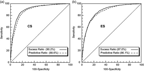
The ROC curve provides us with an approach to evaluate the overall performance of the classification models (Hong et al. 2015b). The area under the ROC curve (AUC) can intuitively express the meaning carried by the ROC curve. Figure 15 displays the ROC curves for CS and ES model. The success rates of the ANN models are 90.2% and 87.0%, and the predictive rates are 88.6% and 86.1%, respectively. Therefore, the models with AUC value both much larger than 50% perform well. Apparently, the CS model is better than the ES model.

Figure 15. ROC curves of CS and ES models: (a) CS and (b) ES.

4.3. Landslide susceptibility maps

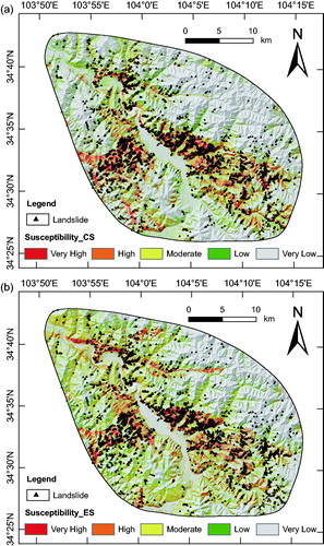
The high classification accuracy and the good performance suggest that the ANN models can be used in the whole study area to map the landslide susceptibility. Combined with the ANN models and control factors in the study area, the susceptibility maps of CS and ES cases were generated. By using the reclassified method of natural breaks, the landslide susceptibility maps were both categorized into five classes: (1) very high; (2) high; (3) moderate; (4) low; and (5) very low. The final landslide susceptibility maps are shown in Figure 16.

Figure 16. Landslide susceptibility maps for cases of (a) CS and (b) ES in the study area.

5. Analyses and discussion

The results of CS case in the entire study area show that there are 5016 (77.42% of the total) landslides distributed in the high and very high categories of the landslide susceptibility map with an area of 140.19 km² (16.04% of the total area); and for the ES case, the high and very high categories with an area of 144.08 km² (accounting for 16.49%) possessed 4621 landslides (accounting for 71.32%) (Figure 17 and Table 2). Compared to the ES case, there are more landslides concentrated in a much smaller area, which is classified as very high and high class in the CS case. This reflects the higher performance of the CS case in the ANN analysis.

Figure 17. Class area and landslide number percentage in each susceptibility class for the cases of CS and ES.

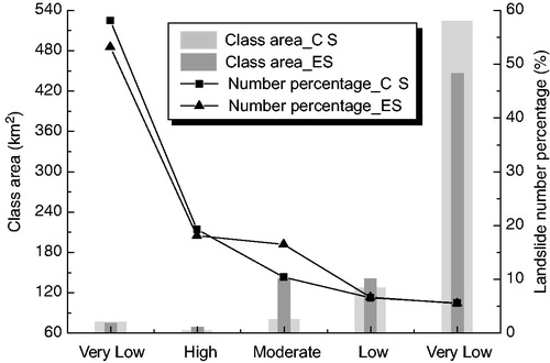
Table 2. Landslide distribution in each susceptibility class.

Susceptibility class	CS model			ES model
	Class area (km^2)	Landslide number	Landslide number percentage (%)	Class area (km^2)	Landslide number	Landslide number percentage (%)
1. Very high	75.77	3765	58.11	75.14	3447	53.20
2. High	64.42	1251	19.31	68.94	1174	18.12
3. Moderate	81.11	675	10.42	141.74	1070	16.51
4. Low	127.95	426	6.58	141.57	431	6.65
5. Very low	524.69	362	5.59	446.56	357	5.51

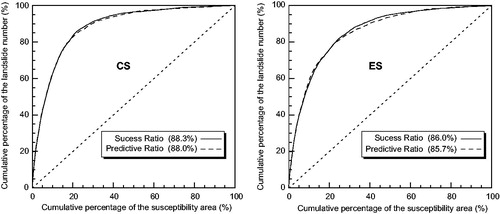
Using the cumulative percentage of the susceptibility area as the abscissa (x-axis) and the cumulative percentage of the landslide number as the ordinate (y-axis), the cumulative percentage curve depicts the quality of the susceptibility map quantitatively (Xu et al. 2016a). Then, the training and testing landslide samples were used to construct the cumulative percentage curves concerning the CS and ES susceptibility maps (Figure 18). The success and predictive ratios of the CS susceptibility map are 88.3% and 88.0%, respectively; and for the ES case, they are 86.0% and 85.7%, respectively. Since the higher success and predictive ratios imply a better susceptibility map, the results show that the two susceptibility maps both largely coincide with the actual landslide distribution in the Minxian earthquake region. Moreover, the CS model considering seismic factors works well. On the other hand, the results also imply that the ANN model is a promising tool in mapping earthquake-induced landslide susceptibility.

Figure 18. Success and predictive ratio curves of the susceptibility maps in the cases of CS and ES.

The quantitative comparison above shows that the CS model performs a little better than the ES model. However, a small bit difference of predictive ratio may mean a big difference of the landslide susceptibility areas (Hong et al. 2015a). Hence, it can be deduced that the seismic factors play a major role in the spatial distribution of landslides triggered by the 2013 Minxian earthquake. To analyse the degree of the difference between the susceptibility maps, the corresponding overlapping areas of each susceptibility class for CS and ES cases were calculated, which represented the same areas predicted by both CS and ES model. According to Table 3, the differences between the two susceptibility maps mainly exist in the high, moderate and low classes. The very high class has a moderate duplication, and the map of the CS case has an area of 40.01 km² (accounting for 52.8%) which was also classified by ES model to be the very high class. The overlapping area with an area of 385.91 km² accounts for 73.55% in the very low class. The higher overlapping percentage of these two classes may indicate that they are relatively prone to landsliding and remaining stable, respectively, no matter whether an earthquake occurred or not. While for the high, moderate and low classes, they may be more subject to the strong ground shaking triggered by an earthquake. Therefore, when mapping the landslide susceptibility without seismic factors, the result is also acceptable.

Table 3. Comparison of each susceptibility class for the CS and ES models.

Susceptibility class	Overlapping area (km^2)	CS model		ES model
		Class area (km^2)	Percentage (%)	Class area (km^2)	Percentage (%)
1. Very high	40.01	75.77	52.80	75.14	53.25
2. High	14.14	64.42	21.95	68.94	20.51
3. Moderate	25.67	81.11	31.65	141.74	18.11
4. Low	26.40	127.95	20.63	141.57	18.65
5. Very low	385.91	524.69	73.55	446.56	86.42

Therefore, despite the moderate duplication, the susceptibility map obtained from the ES model still could provide useful background information for landslide disaster prevention and mitigation, especially for the safe and extreme potential dangerous regions. Generally speaking, the seismic parameters, such as the seismogenic fault, earthquake intensity and PGA, are unknown before an earthquake happens in regions with high seismic risk. To minimize the losses, the disaster prevention should be taken into account in advance. For example, according to the susceptibility map in the ES case, the priority of the infrastructure construction can be developed in the very low susceptibility regions; and the further geotechnical and engineering geological measures should be considered in the very high susceptibility areas.

6. Conclusions

Based on the coseismic landslides inventory of the 2013 Minxian, China Mw5.9 earthquake and ten control factors (elevation, slope angle, slope aspect, curvature, slope position, distance to drainages, lithology, earthquake intensity, peak ground acceleration, and distance to the seismogenic fault), the ANN models were adopted to build the landslide susceptibility maps in the affected area. During this mapping, two cases were considered: one includes all the control factors above (CS Model), and the other excludes the seismic factors (ES model). In the CS case, the success and predictive ratios of the model are 90.2% and 88.6%, respectively; and for the cumulative percentage curve related to the susceptibility map, they are 88.3% and 88.0%, respectively. While in the ES case, the success and predictive ratios of the model are 87.0% and 86.1%, respectively; and for the cumulative percentage curve related to the susceptibility map, they are 86.0% and 85.7%, respectively. Combined with the values, it can be concluded that the ES model has a relatively poor performance. The comparison of the overlapping susceptibility areas shows that 52.8% of the very high susceptibility areas derived from the CS model coincide with the ES model; and for the very low susceptibility areas, the percentage is 73.55%. In spite of the moderate duplication, the susceptibility assessment only using terrain and geological factors can also provide useful background information for taking proper measures before the future earthquakes to reduce the disasters caused by the earthquake-triggered landslides.

Disclosure statement

No potential conflict of interest was reported by the authors.

Additional information

Funding

This research was supported by the National Key Research and Development Program of China [grant number 2017YFB0504104]; National Natural Science Foundation of China [grant number 41661144037]; and Scientific Research Fund of Institute of Engineering Mechanics, China Earthquake Administration [grant number 2017QJGJ05-03].

References

- Bai SB, Wang J, Thiebes B, Cheng C, Chang ZY. 2014. Susceptibility assessments of the Wenchuan earthquake-triggered landslides in Longnan using logistic regression. Environ Earth Sci. 71(2):731–743.
- Chen W, Pourghasemi HR, Zhao Z. 2017a. A GIS-based comparative study of Dempster-Shafer, logistic regression, and artificial neural network models for landslide susceptibility mapping. Geocarto Int. 32(4):367–385.
- Chen W, Xie X, Peng J, Wang J, Duan Z, Hong H. 2017b. GIS-based landslide susceptibility modelling: a comparative assessment of kernel logistic regression, Naïve-Bayes tree, and alternating decision tree models. Geomat Nat Haz Risk. 8(2): 950–973.
- Dai F, Lee CF. 2002. Landslide characteristics and slope instability modeling using GIS, Lantau Island, Hong Kong. Geomorphology. 42(s 3–4):213–228.
- Dai F, Xu C, Yao X, Xu L, Tu X, Gong QM. 2011. Spatial distribution of landslides triggered by the 2008 Ms 8.0 Wenchuan earthquake, China. J Asian Earth Sci. 40(4):883–895.
- Dou J, Tien Bui D, Yunus AP, Jia K, Song X, Revhaug I, Xia H, Zhu Z. 2015a. Optimization of causative factors for landslide susceptibility evaluation using remote sensing and GIS Data in Parts of Niigata, Japan. PloS One. 10(7):e0133262.
- Dou J, Yamagishi H, Pourghasemi HR, Yunus AP, Song X, Xu Y, Zhu Z. 2015b. An integrated artificial neural network model for the landslide susceptibility assessment of Osado Island, Japan. Nat Haz. 78(3):1749–1776.
- Gómez H, Kavzoglu T. 2005. Assessment of shallow landslide susceptibility using artificial neural networks in Jabonosa River Basin, Venezuela. Eng Geol. 78:11–27. doi:https://doi.org/10.1016/j.enggeo.2004.10.004
- Gorum T, Fan X, van Westen CJ, Huang RQ, Xu Q, Tang C, Wang G. 2011. Distribution pattern of earthquake-induced landslides triggered by the 12 May 2008 Wenchuan earthquake. Geomorphology. 133(3):152–167.
- Gorum T, van Westen CJ, Korup O, van der Meijde M, Fan X, van der Meer FD. 2013. Complex rupture mechanism and topography control symmetry of mass-wasting pattern, 2010 Haiti earthquake. Geomorphology. 184:127–138.
- Guzzetti F, Reichenbach P, Ardizzone F, Cardinali M, Galli M. 2006. Estimating the quality of landslide susceptibility models. Geomorphology. 81(1):166–184.
- He W, Zheng W, Wang A, Liu X, Zhang B, Liu F, Pang W. 2013. New activities of Lintan-Dangchang fault and ite relations to Minxian-Zhangxian Ms 6.6 earthquake. China Earthquake Eng J. 35(4):751–760. (in Chinese)
- Hong H, Pradhan B, Xu C, Tien Bui D. 2015a. Spatial prediction of landslide hazard at the Yihuang area (China) using two-class kernel logistic regression, alternating decision tree and support vector machines. CATENA. 133:266–281.
- Hong H, Xu C, Revhaug I, Bui DT. 2015b. Spatial prediction of landslide hazard at the Yihuang area (China): a comparative study on the predictive ability of backpropagation multi-layer perceptron neural networks and radial basic function neural networks. In: Robbi Sluter C, Madureira Cruz CB, Leal de Menezes PM, editors. Cartography – Maps Connecting the World: 27th International Cartographic Conference 2015 – ICC2015. Brazil: Springer International Publishing; p. 175–188.
- Hong H, Pourghasemi HR, Pourtaghi ZS. 2016a. Landslide susceptibility assessment in Lianhua County (China): a comparison between a random forest data mining technique and bivariate and multivariate statistical models. Geomorphology. 259:105–118.
- Hong H, Pradhan B, Jebur MN, Bui DT, Xu C, Akgun A. 2016b. Spatial prediction of landslide hazard at the Luxi area (China) using support vector machines. Environ Earth Sci. 75(1):40.
- Hong H, Chen W, Xu C, Youssef AM, Pradhan B, Tien Bui D. 2017a. Rainfall-induced landslide susceptibility assessment at the Chongren area (China) using frequency ratio, certainty factor, and index of entropy. Geocarto Int. 32(2):139–154.
- Hong H, Ilia I, Tsangaratos P, Chen W, Xu C. 2017b. A hybrid fuzzy weight of evidence method in landslide susceptibility analysis on the Wuyuan area, China. Geomorphology. 290:1–16.
- Jenness J, Brost B, Beier P. 2013. Land Facet Corridor Designer: Extension for ArcGIS. Jenness Enterprises. Available at: http://www.jennessent.com/arcgis/land_facets.htm
- Kamp U, Growley BJ, Khattak GA, Owen LA. 2008. GIS-based landslide susceptibility mapping for the 2005 Kashmir earthquake region. Geomorphology. 101(4):631–642.
- Kamp U, Owen LA, Growley BJ, Khattak GA. 2010. Back analysis of landslide susceptibility zonation mapping for the 2005 Kashmir earthquake: an assessment of the reliability of susceptibility zoning maps. Nat Haz. 54(1):1–25.
- Keefer DK. 2000. Statistical analysis of an earthquake-induced landslide distribution – The 1989 Loma Prieta, California event. Eng Geol. 58(3-4):231–249.
- Lee C. 2014. Statistical seismic landslide hazard analysis: an example from Taiwan. Eng Geol. 182:201–212.
- Lee S, Ryu J-H, Min K, Won J-S. 2003. Landslide susceptibility analysis using GIS and artificial neural network. Earth Surf Proc Land. 28(12):1361–1376.
- Lee S, Ryu J-H, Won J-S, Park H-J. 2004. Determination and application of the weights for landslide susceptibility mapping using an artificial neural network. Eng Geol. 71(3-4):289–302.
- Lee S, Ryu J-H, Kim I-S. 2007. Landslide susceptibility analysis and its verification using likelihood ratio, logistic regression, and artificial neural network models: case study of Youngin, Korea. Landslides. 4(4):327–338.
- Lee S, Jeon Seong W, Oh K-Y, Lee M-J. 2016. The spatial prediction of landslide susceptibility applying artificial neural network and logistic regression models: a case study of Inje, Korea. Open Geosci. 8(1):117–132.
- Lee S, Hong S-M, Jung H-S. 2017. A support vector machine for landslide susceptibility mapping in Gangwon Province, Korea. Sustainability. 9(1):48.
- Parker RN, Densmore AL, Rosser NJ, de Michele M, Li Y, Huang R, Whadcoat S, Petley DN. 2011. Mass wasting triggered by the 2008 Wenchuan earthquake is greater than orogenic growth. Nat Geosci. 4(7):449–452.
- Pradhan B, Lee S. 2009. Regional landslide susceptibility analysis using back-propagation neural network model at Cameron Highland, Malaysia. Landslides. 7(1):13–30.
- Pradhan B, Lee S. 2010. Landslide susceptibility assessment and factor effect analysis: backpropagation artificial neural networks and their comparison with frequency ratio and bivariate logistic regression modelling. Environ Model Softw. 25(6):747–759.
- Rao G, Cheng Y, Lin A, Yan B. 2017. Relationship between landslides and active normal faulting in the epicentral area of the AD 1556 M∼8.5 Huaxian Earthquake, SE Weihe Graben (Central China). J Earth Sci. 28(3):545–554.
- Regmi AD, Devkota KC, Yoshida K, Pradhan B, Pourghasemi HR, Kumamoto T, Akgun A. 2013. Application of frequency ratio, statistical index, and weights-of-evidence models and their comparison in landslide susceptibility mapping in Central Nepal Himalaya. Arab J Geosc. 7(2):725–742.
- Ripley BD. 1996. Pattern recognition and neural networks. New York: Cambridge University Press.
- Tian Y, Xu C, Xu X, Chen J. 2016. Detailed inventory mapping and spatial analyses to landslides induced by the 2013 Ms 6.6 Minxian Earthquake of China. J Earth Sci. 27(6):1016–1026.
- Tian Y, Xu C, Chen J, Hong H. 2017a. Spatial distribution and susceptibility analyses of pre-earthquake and coseismic landslides related to the Ms 6.5 earthquake of 2014 in Ludian, Yunan, China. Geocarto Int. 32(9):978–989.
- Tian Y, Xu C, Chen J, Zhou Q, Shen L. 2017b. Geometrical characteristics of earthquake-induced landslides and correlations with control factors: a case study of the 2013 Minxian, Gansu, China, Mw 5.9 event. Landslides. Doi: 10.1007/s10346-017-0835-6
- Tien Bui D, Lofman O, Revhaug I, Dick O. 2011. Landslide susceptibility analysis in the Hoa Binh province of Vietnam using statistical index and logistic regression. Nat Haz. 59(3):1413.
- Tien Bui D, Pradhan B, Lofman O, Revhaug I, Dick OB. 2012a. Landslide susceptibility assessment in the Hoa Binh province of Vietnam: a comparison of the Levenberg–Marquardt and Bayesian regularized neural networks. Geomorphology. 171–172(6):12–29.
- Tien Bui D, Pradhan B, Lofman O, Revhaug I, Dick OB. 2012b. Landslide susceptibility mapping at Hoa Binh province (Vietnam) using an adaptive neuro-fuzzy inference system and GIS. Comput Geosci. 45:199–211.
- Tien Bui D, Pradhan B, Revhaug I, Nguyen DB, Pham HV, Bui QN. 2013. A novel hybrid evidential belief function-based fuzzy logic model in spatial prediction of rainfall-induced shallow landslides in the Lang Son city area (Vietnam). Geomat Nat Haz Risk. 6(3):243–271.
- Tien Bui D, Tuan TA, Klempe H, Pradhan B, Revhaug I. 2016. Spatial prediction models for shallow landslide hazards: a comparative assessment of the efficacy of support vector machines, artificial neural networks, kernel logistic regression, and logistic model tree. Landslides. 13(2):361–378.
- Tien Bui D, Bui Q-T, Nguyen Q-P, Pradhan B, Nampak H, Trinh PT. 2017. A hybrid artificial intelligence approach using GIS-based neural-fuzzy inference system and particle swarm optimization for forest fire susceptibility modeling at a tropical area. Agricul For Meteorol. 233:32–44.
- Wang H, Liu G, Xu W, Wang G. 2005. GIS-based landslide hazard assessment: an overview. Prog Phys Geogr. 29(4): 548–567.
- Wang Y, Song C, Lin Q, Li J. 2016. Occurrence probability assessment of earthquake-triggered landslides with Newmark displacement values and logistic regression: The Wenchuan earthquake, China. Geomorphology. 258:108–119.
- Weiss A. Topographic position and landforms analysis. Poster presentation, ESRI User Conference, San Diego, CA; 2001.
- Xu C. 2015. Preparation of earthquake-triggered landslide inventory maps using remote sensing and GIS technologies: principles and case studies. Geosci Front. 6(6):825–836.
- Xu C, Xu X. 2013. Controlling parameter analyses and hazard mapping for earthquake-triggered landslides: an example from a square region in Beichuan County, Sichuan Province, China. Arab J Geosci. 6(10):3827–3839.
- Xu C, Xu X. 2014. The spatial distribution pattern of landslides triggered by the 20 April 2013 Lushan earthquake of China and its implication to identification of the seismogenic fault. Chinese Sci Bull. 59(13):1416–1424.
- Xu C, Dai F, Xu X, Lee YH. 2012a. GIS-based support vector machine modeling of earthquake-triggered landslide susceptibility in the Jianjiang River watershed, China. Geomorphology. 145-146:70–80.
- Xu C, Xu X, Dai F, Xiao J, Tan X, Yuan R. 2012b. Landslide hazard mapping using GIS and weight of evidence model in Qingshui River watershed of 2008 Wenchuan earthquake struck region. J Earth Sci. 23(1):97–120.
- Xu C, Xu X, Dai F, Wu Z, He H, Shi F, Wu X, Xu S. 2013a. Application of an incomplete landslide inventory, logistic regression model and its validation for landslide susceptibility mapping related to the May 12, 2008 Wenchuan earthquake of China. Nat Haz. 68(2):883–900.
- Xu C, Xu X, Yao Q, Wang Y. 2013b. GIS-based bivariate statistical modelling for earthquake-triggered landslides susceptibility mapping related to the 2008 Wenchuan earthquake, China. Quart J Eng Geol Hydrogeol. 46(2):221–236.
- Xu C, Xu X, Yu G. 2013c. Landslides triggered by slipping-fault-generated earthquake on a plateau: an example of the 14 April 2010, Ms 7.1, Yushu, China earthquake. Landslides. 10(4):421–431.
- Xu C, Shyu JBH, Xu X. 2014a. Landslides triggered by the 12 January 2010 Port-au-Prince, Haiti, Mw =7.0 earthquake: visual interpretation, inventory compiling, and spatial distribution statistical analysis. Nat Haz Earth Syst Sci. 14(7):1789–1818.
- Xu C, Xu X, Dai F, Yao X. 2014b. Three (nearly) complete inventories of landslides triggered by the May 12, 2008 Wenchuan Mw 7.9 earthquake of China and their spatial distribution statistical analysis. Landslides. 11(3):441–461.
- Xu C, Xu X, Shyu JBH. 2015a. Database and spatial distribution of landslides triggered by the Lushan, China Mw 6.6 earthquake of 20 April 2013. Geomorphology. 248:77–92.
- Xu C, Xu X, Shyu JBH, Gao M, Tan X, Ran Y, Zheng W. 2015b. Landslides triggered by the 20 April 2013 Lushan, China, Mw 6.6 earthquake from field investigations and preliminary analyses. Landslides. 12(2):365–385.
- Xu C, Shen L, Wang G. 2016a. Soft computing in assessment of earthquake-triggered landslide susceptibility. Environ Earth Sci. 75(9): 767.
- Xu C, Xu X, Shen L, Yao Q, Tan X, Kang W, Ma S, Wu X, Cai J, Gao M et al. 2016b. Optimized volume models of earthquake-triggered landslides. Sci Rep. [accessed 2016]:[29797 p.]. doi:10.1038/srep29797.
- Xu C, Xu X, Tian Y, Shen L, Yao Q, Huang X, Ma J. 2016c. Two Comparable Earthquakes Produced Greatly Different Coseismic Landslides: The 2015 Gorkha, Nepal and 2008 Wenchuan, China Events. J Earth Sci. 27(6):1008–1015.
- Xu C, Tian Y, Zhou B, Ran H, Lyu G. 2017. Landslide damage along Araniko highway and Pasang Lhamu highway and regional assessment of landslide hazard related to the Gorkha, Nepal earthquake of 25 April 2015. Geoenviron Disasters. 4(1):14.
- Yesilnacar E, Topal T. 2005. Landslide susceptibility mapping: a comparison of logistic regression and neural networks methods in a medium scale study, Hendek region (Turkey). Eng Geol. 79(3-4):251–266.
- Yilmaz I. 2009a. A case study from Koyulhisar (Sivas-Turkey) for landslide susceptibility mapping by artificial neural networks. Bull Eng Geol Environ. 68(3):297–306.
- Yilmaz I. 2009b. Landslide susceptibility mapping using frequency ratio, logistic regression, artificial neural networks and their comparison: a case study from Kat landslides (Tokat—Turkey). Comput Geosci. 35(6):1125–1138.
- Yilmaz I. 2010. Comparison of landslide susceptibility mapping methodologies for Koyulhisar, Turkey: conditional probability, logistic regression, artificial neural networks, and support vector machine. Environ Earth Sci. 61(4):821–836.
- Yin Y, Wang F, Sun P. 2009. Landslide hazards triggered by the 2008 Wenchuan earthquake, Sichuan, China. Landslides. 6(2):139–152.