Stability reliability of a cutting slope in Laohuzui Hydropower Station in Tibet of China

Abstract

The Hoek–Brown empirical formulas are widely used to estimate the mechanical parameters of a rock mass. However, there exists a problem of variability and uncertainty in the mechanical parameters of a rock mass estimated by the Hoek–Brown empirical formulas. To do this, we present a method to implement a reliability analysis of the rock mass stability directly starting with the basic variables of the Hoek–Brown empirical formulas. First, a quantitative assessment of the disturbance factor is recommended to overcome the subjectivity and limitation of estimating the disturbance factor according to the guidelines by Hoek et al. Second, a performance function is built up together with the safety factor of a micro-unit. Third, the Rosenblueth point estimate method is chosen to estimate the mean and standard deviation of the factor of safety. Finally, the stability reliability of a cutting slope in Laohuzui Hydropower Station in Tibet of China is analyzed. The results of the cutting slope show good agreement with the rock mass failure that occurred.

Keywords:

• Hoek–Brown empirical formulas
• reliability assessment
• factor of safety
• Rosenblueth point estimate method

1. Introduction

Although the reliability assessment methods have been applied to the field of rock engineering (Harr 1987; Wiles 2006; Lu et al. 2013; Johari et al. 2013; Lu et al. 2017), the basic problem existing in the stability analysis of a rock mass is how to rationally and reliably assess the mechanical parameters (Lin et al. 2013; Rajesh et al. 2013; Wei et al. 2018). In general, the mechanical properties of a rock mass cannot be directly characterized by the laboratory test results of intact rocks, whereas they can be exactly evaluated through an in-situ test or back-analysis (Edelbro 2004; Taheri and Tani 2010; Fernandez-Rodriguez et al. 2014). However, just considering the construction of hydropower projects in China, the in-situ test is usually used in large hydropower projects and the number of tests is low. The limited test data cannot meet the statistical requirements. In particular, the in-situ test is not carried out in many small hydropower projects owing to its high cost and operational difficulty. Furthermore, the back-analysis is applicable only to situations in which failure has occurred or prototype observation data have been obtained. Therefore, empirical methods are often adopted to assess the mechanical parameters of a rock mass in many projects (Hoek et al. 2002; Wang et al. 2011; Vasarhelyi and Kovacs 2016; Kayabasi and Gokceoglu 2018).

Among the empirical methods, the Hoek–Brown empirical method is widely used to estimate the mechanical parameter values of a rock mass (Hoek et al. 2002). However, the basic parameters of the Hoek–Brown empirical formulas are usually variable and uncertain (Hoek 1998). As a result, a problem of variability and uncertainty in the mechanical parameters of a rock mass estimated by the Hoek–Brown empirical formulas still exists. If the basic parameters of the Hoek–Brown empirical formulas are considered to be deterministic, limitations will exist in the stability assessment of a rock mass. Conversely, if their probability distributions are considered, then the probability of failure and the risk level can be evaluated through a reliability analysis. However, it has not been reported how to implement a reliability analysis of rock mass stability directly starting with the basic variables of the Hoek–Brown empirical formulas. For this reason, after briefly introducing the Hoek–Brown empirical formulas, this study develops four aspects, summarized as follows:

1. Analysis of the subjectivity and limitation of estimating the disturbance factor of the Hoek–Brown empirical formulas, proposing the concept of a generalized disturbance factor applicable to a non-excavated rock mass, and recommending a method to evaluate the disturbance factor quantitatively.

2. According to the rock mass stresses, definition of the factor of safety of a micro-unit, and then establishment of a performance function in which the basic variables of the Hoek–Brown empirical formulas are contained.

3. Selection of the Rosenblueth point estimate method to calculate the mean and standard deviation of the factor of safety of the element, discussing how to combine the Rosenblueth point estimate method with the finite element method in detail, and suggesting the calculation procedure of the reliability index for two and more Hoek–Brown rock masses.

4. Finally, analysis of the stability reliability of a cutting slope, comparing the calculation results with the failure that occurred, and demonstrating the rationality of the designed anchorage-cable length.

In this study, a cutting slope at the Laohuzui Hydropower Station in Tibet will be used as an example to illustrate the process of reliability analysis using the proposed method.

2. Assessment method of the disturbance factor in Hoek–Brown formulas

2.1. Hoek–Brown formulas

Hoek et al. (2002) introduced a method to estimate mechanical parameters using the Hoek–Brown empirical formulas, and the rock mass strengths could be derived by (1) $${{\sigma }^{\prime }}_1={{\sigma }^{\prime }}_3+{\sigma }_{\text{ci}}{\left(m_{\mathrm{b}}\frac{{{\sigma }^{\prime }}_3}{{\sigma }_{\text{ci}}}+s\right)}^{\alpha }$$(1) where ${{\sigma }^{\prime }}_1$ and ${{\sigma }^{\prime }}_3$ are the major and minor effective principal stresses at failure of the rock mass, respectively (note that the compressive stress is taken as positive); σ_ci is the uniaxial compressive strength of intact rock; and m_b, s, and α are the material constants related to the rock mass properties (Equations (2)–(4)). (2) $$m_{\mathrm{b}}=m_{\mathrm{i}}\times \hspace{0.17em}\text{exp}\hspace{0.17em}\left(\frac{\text{GSI}-100}{28-14D}\right)$$(2) (3) $$s=\hspace{0.17em}\text{exp}\hspace{0.17em}\left(\frac{\text{GSI}-100}{9-3D}\right)$$(3) (4) $$\alpha =\frac{1}{2}+\frac{1}{6}\left(\hspace{0.17em}\text{exp}\hspace{0.17em}\left(-\frac{\text{GSI}}{15}\right)-\hspace{0.17em}\text{exp}\hspace{0.17em}\left(-\frac{20}{3}\right)\right)$$(4)

According to Equation (1)(1) $${{\sigma }^{\prime }}_1={{\sigma }^{\prime }}_3+{\sigma }_{\text{ci}}{\left(m_{\mathrm{b}}\frac{{{\sigma }^{\prime }}_3}{{\sigma }_{\text{ci}}}+s\right)}^{\alpha }$$(1) , the tensile strength σ_t, uniaxial compressive strength σ_c, global strength ${{\sigma }^{\prime }}_{\text{cm}}$, equivalent angle of friction φ′, and cohesive strength c′ of the rock mass can be obtained, as in Equations (5)–(9), respectively. (5) $${\sigma }_{\mathrm{t}}=-\frac{s{\sigma }_{\text{ci}}}{m_{\mathrm{b}}}$$(5) (6) $${\sigma }_{\mathrm{c}}={\sigma }_{\text{ci}}{s}^{\alpha }$$(6) (7) $${{\sigma }^{\prime }}_{\text{cm}}={\sigma }_{\text{ci}}\times \frac{\left(m_{\mathrm{b}}+4s-a(m_{\mathrm{b}}-8s)\right)\times {(m_{\mathrm{b}}/(4+s\left)\right)}^{a-1}}{2(1+a)(2+a)}$$(7) (8) $${\varphi }^{\prime }={\hspace{0.17em}\text{sin}\hspace{0.17em}}^{-1}\left[\frac{6a{m}_{\mathrm{b}}{\left(s+m_{\mathrm{b}}{{\sigma }^{\prime }}_{3\mathrm{n}}\right)}^{a-1}}{2(1+a)(2+a)+6a{m}_{\mathrm{b}}{\left(s+m_{\mathrm{b}}{{\sigma }^{\prime }}_{3\mathrm{n}}\right)}^{a-1}}\right]$$(8) (9) $$c^{\prime }=\frac{{\sigma }_{\text{ci}}\left[(1+2a)s+(1-a)m_{\mathrm{b}}{{\sigma }^{\prime }}_{3\mathrm{n}}\right]{\left(s+m_{\mathrm{b}}{{\sigma }^{\prime }}_{3\mathrm{n}}\right)}^{a-1}}{(1+a)(2+a)\sqrt{1+\frac{\left(6a{m}_{\mathrm{b}}{\left(s+m_{\mathrm{b}}{{\sigma }^{\prime }}_{3\mathrm{n}}\right)}^{a-1}\right)}{(1+a)(2+a)}}}$$(9)

The tensile strength σ_t in Equation (5)(5) $${\sigma }_{\mathrm{t}}=-\frac{s{\sigma }_{\text{ci}}}{m_{\mathrm{b}}}$$(5) is taken as negative. The uniaxial compressive strength σ_c in Equation (6)(6) $${\sigma }_{\mathrm{c}}={\sigma }_{\text{ci}}{s}^{\alpha }$$(6) is taken as positive. The variable ${{\sigma }^{\prime }}_{3\mathrm{n}}$ in Equations (8)(8) $${\varphi }^{\prime }={\hspace{0.17em}\text{sin}\hspace{0.17em}}^{-1}\left[\frac{6a{m}_{\mathrm{b}}{\left(s+m_{\mathrm{b}}{{\sigma }^{\prime }}_{3\mathrm{n}}\right)}^{a-1}}{2(1+a)(2+a)+6a{m}_{\mathrm{b}}{\left(s+m_{\mathrm{b}}{{\sigma }^{\prime }}_{3\mathrm{n}}\right)}^{a-1}}\right]$$(8) and (9)(9) $$c^{\prime }=\frac{{\sigma }_{\text{ci}}\left[(1+2a)s+(1-a)m_{\mathrm{b}}{{\sigma }^{\prime }}_{3\mathrm{n}}\right]{\left(s+m_{\mathrm{b}}{{\sigma }^{\prime }}_{3\mathrm{n}}\right)}^{a-1}}{(1+a)(2+a)\sqrt{1+\frac{\left(6a{m}_{\mathrm{b}}{\left(s+m_{\mathrm{b}}{{\sigma }^{\prime }}_{3\mathrm{n}}\right)}^{a-1}\right)}{(1+a)(2+a)}}}$$(9) is equals to ${{\sigma }^{\prime }}_{3\max }/{\sigma }_{\text{ci}}$, and ${{\sigma }^{\prime }}_{3\max }$ is the upper limit of the confining stress when fitting the linear Mohr–Coulomb equation. Hoek et al. (2002) provided equations calculating ${{\sigma }^{\prime }}_{3\max }$ for slopes and tunnels (Hoek et al. 2002).

Furthermore, the rock mass modulus of deformation E_m can be estimated by Equation (10)(10) $$\{\begin{array}{ll}{E}_{\mathrm{m}}=\left(1-\frac{D}{2}\right)\sqrt{\frac{{\sigma }_{\text{ci}}}{100}}\times {10}^{\frac{\text{GSI}-10}{40}}& ({\sigma }_{\text{ci}}\le 100\text{MPa})\\ E_{\mathrm{m}}=\left(1-\frac{D}{2}\right)\times {10}^{\frac{\text{GSI}-10}{40}}& ({\sigma }_{\text{ci}}>100\text{MPa})\end{array}$$(10) . It should be noted that the unit of modulus is GPa in Equation (10)(10) $$\{\begin{array}{ll}{E}_{\mathrm{m}}=\left(1-\frac{D}{2}\right)\sqrt{\frac{{\sigma }_{\text{ci}}}{100}}\times {10}^{\frac{\text{GSI}-10}{40}}& ({\sigma }_{\text{ci}}\le 100\text{MPa})\\ E_{\mathrm{m}}=\left(1-\frac{D}{2}\right)\times {10}^{\frac{\text{GSI}-10}{40}}& ({\sigma }_{\text{ci}}>100\text{MPa})\end{array}$$(10) . (10) $$\{\begin{array}{ll}{E}_{\mathrm{m}}=\left(1-\frac{D}{2}\right)\sqrt{\frac{{\sigma }_{\text{ci}}}{100}}\times {10}^{\frac{\text{GSI}-10}{40}}& ({\sigma }_{\text{ci}}\le 100\text{MPa})\\ E_{\mathrm{m}}=\left(1-\frac{D}{2}\right)\times {10}^{\frac{\text{GSI}-10}{40}}& ({\sigma }_{\text{ci}}>100\text{MPa})\end{array}$$(10)

From the above equations, we can see that it is very easy to calculate the mechanical parameter values of a rock mass with the Hoek–Brown empirical formulas when the values of the basic variables geological strength index (GSI), D, σ_ci, and m_i are determined.

The GSI is related to the rock mass structures and conditions of the surfaces of discontinuity, and its value ranges from 0 to 100.

The disturbance factor D reflects the degree of influence to which the rock mass has been subjected as a result of blast damage and stress relaxation owing to excavation. In consideration of the fact that the mechanical parameter values of the rock mass may be overestimated using the previous Hoek–Brown criterion, the disturbance factor D was introduced in the 2002 edition and it varies from 0 to 1. For more details, see the guidelines proposed by Hoek et al. (2002).

The uniaxial compressive strength σ_ci and material parameter m_i of intact rock can be assessed according to the laboratory triaxial test results and the method introduced by Hoek and Karakas (2008). If the laboratory triaxial test is not carried out, the empirical values of σ_ci and m_i can be selected (Hoek and Karakas 2008). However, the uniaxial compressive strength and tensile strength of intact rock can be easily tested in the laboratory. When the compressive strength and tensile strength are obtained, the material parameter m_i can be acquired by Equation (1)(1) $${{\sigma }^{\prime }}_1={{\sigma }^{\prime }}_3+{\sigma }_{\text{ci}}{\left(m_{\mathrm{b}}\frac{{{\sigma }^{\prime }}_3}{{\sigma }_{\text{ci}}}+s\right)}^{\alpha }$$(1) . We know that GSI equals 100 and D equals 0 for intact rock. Setting GSI =100 and D = 0 in Equation (1)(1) $${{\sigma }^{\prime }}_1={{\sigma }^{\prime }}_3+{\sigma }_{\text{ci}}{\left(m_{\mathrm{b}}\frac{{{\sigma }^{\prime }}_3}{{\sigma }_{\text{ci}}}+s\right)}^{\alpha }$$(1) , then (11) $${{\sigma }^{\prime }}_1={{\sigma }^{\prime }}_3+{\sigma }_{\text{ci}}{\left(m_{\mathrm{i}}\frac{{{\sigma }^{\prime }}_3}{{\sigma }_{\text{ci}}}+1\right)}^{0.5}$$(11)

It should be noted that the tensile strength of intact rock is negative and the stress state corresponding to the condition of uniaxial tension is ${{\sigma }^{\prime }}_1=100$ and ${{\sigma }^{\prime }}_3={\sigma }_{\text{ti}}$. Substituting them into Equation (11)(11) $${{\sigma }^{\prime }}_1={{\sigma }^{\prime }}_3+{\sigma }_{\text{ci}}{\left(m_{\mathrm{i}}\frac{{{\sigma }^{\prime }}_3}{{\sigma }_{\text{ci}}}+1\right)}^{0.5}$$(11) , then (12) $$m_{\mathrm{i}}=\frac{{\sigma }_{\text{ti}}^2-{\sigma }_{\text{ci}}^2}{{\sigma }_{\text{ci}}\times {\sigma }_{\text{ti}}}$$(12)

2.2. Subjectivity and limitation of the existing method for evaluating the disturbance factor

According to the geological exploration and rock mechanics test results, the reasonable intervals of GSI, σ_ci, and m_i may be easily determined. Owing to the subjectivity of professional technicians, however, the disturbance factor has a significant error because of the subjectivity of professional technicians. For example, Edelbro (2004) analyzed the values of D estimated by 11 professional technicians for the same grade rock mass of the Swedish Laisvall mine (Edelbro 2004). In terms of his analysis, the disturbance factor D ranges from 0 to 0.7, and its mean, standard deviation, and coefficient of variation are 0.28, 0.24 and 0.89 respectively.

In addition to the above-mentioned subjective error, the authors of this article consider that it is also worth discussing the assessment of the disturbance factor in the following two cases:

1. The disturbance factor is also used for a rock mass far from the excavation face. However, this does not conform to the actual situation, because the disturbed rock mass caused by blasting damage and stress relaxation is limited.

2. The disturbance factor is not considered in a non-excavated rock mass. Again, this does not conform to the situation in which the unloading of rock masses has occurred in the natural valley slopes of the mountain gorge area owing to river incision.

Obviously, to eliminate as much as possible the errors caused by subjective judgement and take into account the above two cases, it is necessary to quantitatively assess the disturbance factor by other means.

2.3. Quantitative assessment of disturbance factor

According to the above analysis, we think that the disturbance influence on a non-excavated rock mass, such as the natural valley slopes of a mountain gorge area owing to river incision, should be considered. Otherwise, the mechanical parameter values of the non-excavated rock mass will also be overestimated. For this reason, this work proposes the generalized disturbance factor which may be quantitatively evaluated with the integrity coefficient and can be easily obtained by sonic wave or seismic wave testing (Gao 2012). The generalized disturbance factor is given by (13) $$D=1-K_{\mathrm{v}}$$(13) where K_v is the integrity coefficient of the rock mass and $K_{\mathrm{v}}={(V_{\text{pm}}/V_{\text{pr}})}^2$; V_pm is longitudinal wave velocity of the rock mass, which can be tested by the sonic or seismic methods; V_pr is longitudinal wave velocity of the fresh rock, and it can be replaced using the maximum value of the longitudinal wave velocities measured in the fresh rock mass (Gao 2012).

To demonstrate the feasibility of the above method, this study analyzes the basic data and in-situ test results of the Laohuzui Hydropower Station. The Laohuzui Hydropower Station is located on the Bahe River, a branch of the Yalu Tsangpo River in Tibet, China. The designed water-retaining structure is a gravity dam whose height is 84 m. The lithologies of the dam site are metamorphic quartz sandstone and sandy slate, and the latter accounts for ∼9.4% of the total thickness of the formation. The uniaxial compressive strength and tensile strength are tested in the laboratory for borehole cores. The material parameter m_i is calculated through Equation (12)(12) $$m_{\mathrm{i}}=\frac{{\sigma }_{\text{ti}}^2-{\sigma }_{\text{ci}}^2}{{\sigma }_{\text{ci}}\times {\sigma }_{\text{ti}}}$$(12) . Their respective mean values are listed in Tables 1 and 2.

Table 1. The Values of deformation modulus measured by in-situ tests and estimated by Hoek–Brown empirical formulas.

No.	Adit no.	Testing position (m)	Vpm (m·s^–1)	Kv	D	σci (MPa)	mi	GSI	Test values	Estimated values with H-B Formula
									E0 (GPa)	Em (GPa)
E1-1	PD1	18.2	1945	0.128	0.872	124.88	19.04	35	2.333	2.378
E1-2	PD1	27.3	2370	0.191	0.809	124.88	19.04	45	4.411	4.466
E2	PD2	18.7	1555	0.082	0.918	124.88	19.04	35	2.038	2.281
E3	PD3	17.5	1565	0.083	0.917	124.88	19.04	35	2.213	2.283

Notes: (1) V_pr of intact rock is 5430 m·s^–1, tested by the sonic method in the laboratory; (2) V_pm of rock mass is the average of test results; (3) E₀ is the last cycle test value; (4) GSI, σ_ci, D, and m_i are the average based on basic data; (5) integrity coefficient K_v is the square of the velocity ratio, that is, K_v = (V_pm/V_pm)².

Table 2. The values of the shear strength parameters measured by in-situ tests and estimated by Hoek–Brown failure criterion.

No.	Adit no.	Testing position (m)	Vpm (m·s^–1)	Kv	D	σci (MPa)	mi	GSI	Test values		Estimated values with H-B formula
									φ′ (°)	c′ (MPa)	φ′ (°)	c′ (MPa)
S1	PD1	21.0-40.8	2485	0.209	0.791	124.88	19.04	45	47.91	0.792	50.13	0.646
S2	PD2	20.3-40.6	2153	0.157	0.843	124.88	19.04	45	47.64	0.790	47.82	0.594
S3	PD3	20.5-34.8	1920	0.125	0.875	124.88	19.04	45	44.16	0.862	48.53	0.612

Notes: (1) V_pr of intact rock is 5430 m·s^–1, tested by the sonic method in the laboratory; (2) V_pm of rock mass is the average of test results; (3) φ′ and c′ are the peak values of the test; (4) GSI, σ_ci, D, and m_i are the average based on basic data; (5) integrity coefficient K_v is the square of the velocity ratio, thatis, K_v = (V_pm/V_pm)².

The in-situ tests, carried out in exploration adits of the dam site, include four deformation test sets and three shear test sets. In addition, the seismic wave is also measured on both wall sides of the exploration adit. The test results are also summarized in Tables 1 and 2. The deformation test adopts the rigid-bearing plate method. The bearing plate is 40 cm in diameter and 3 cm in thickness. The loading and unloading cycles are five in total. The pressures corresponding to each cycle are 1.214, 2.427, 3.641, 4.854, and 6.068 MPa, respectively. The bottom of each shear test sample is a square with 50 cm in side length. Each shear test set includes five test points, and the five normal pressures are 0.497, 0.994, 1.491, 1.988, and 2.485 MPa, respectively.

The values of GSI in Tables 1 and 2 are estimated according to the rock mass structures and conditions of the surfaces of discontinuity exposed to the exploration adit. The values of D in Tables 1 and 2 are determined according to the longitudinal wave velocity measured on both wall sides of the exploration adit. The values of E_m in Table 1 are calculated by Equation (10)(10) $$\{\begin{array}{ll}{E}_{\mathrm{m}}=\left(1-\frac{D}{2}\right)\sqrt{\frac{{\sigma }_{\text{ci}}}{100}}\times {10}^{\frac{\text{GSI}-10}{40}}& ({\sigma }_{\text{ci}}\le 100\text{MPa})\\ E_{\mathrm{m}}=\left(1-\frac{D}{2}\right)\times {10}^{\frac{\text{GSI}-10}{40}}& ({\sigma }_{\text{ci}}>100\text{MPa})\end{array}$$(10) . The empirical method used to estimate φ′ and c′ in Table 2 is based on the Hoek–Brown failure criterion, and it is explained as follows.

For the relationship between the normal and the shear stresses of Equation (1)(1) $${{\sigma }^{\prime }}_1={{\sigma }^{\prime }}_3+{\sigma }_{\text{ci}}{\left(m_{\mathrm{b}}\frac{{{\sigma }^{\prime }}_3}{{\sigma }_{\text{ci}}}+s\right)}^{\alpha }$$(1) , Hoek et al. (2002) introduced Balmer’s equations (Balmer 1952), and Priest (2005) adopted the difference formula (Priest 2005). The authors of this article derived the expressions (Equations (14)(14) $$\frac{{\sigma }_{\mathrm{n}}}{{\sigma }_{\text{ci}}}=\frac{1}{m_{\mathrm{b}}}{\left(\frac{2}{m_{\mathrm{b}}a}\right)}^{\frac{1}{a-1}}{\left(\frac{\hspace{0.17em}\text{sin}\hspace{0.17em}{\varphi }_i}{1-\hspace{0.17em}\text{sin}\hspace{0.17em}{\varphi }_i}\right)}^{\frac{1}{a-1}}\left(\frac{\hspace{0.17em}\text{sin}\hspace{0.17em}{\varphi }_i}{a}+1\right)-\frac{s}{m_{\mathrm{b}}}$$(14) and (15)(15) $$\frac{{\tau }_{\mathrm{s}}}{{\sigma }_{\text{ci}}}=\left(\frac{\hspace{0.17em}\text{cos}\hspace{0.17em}{\varphi }_i}{2}\right){\left(\frac{2}{m_{\mathrm{b}}a}\right)}^{\frac{a}{a-1}}{\left(\frac{\hspace{0.17em}\text{sin}\hspace{0.17em}{\varphi }_i}{1-\hspace{0.17em}\text{sin}\hspace{0.17em}{\varphi }_i}\right)}^{\frac{a}{a-1}}$$(15) ) of normal stress σ_n and shear stress τ_s (Appendix A). (14) $$\frac{{\sigma }_{\mathrm{n}}}{{\sigma }_{\text{ci}}}=\frac{1}{m_{\mathrm{b}}}{\left(\frac{2}{m_{\mathrm{b}}a}\right)}^{\frac{1}{a-1}}{\left(\frac{\hspace{0.17em}\text{sin}\hspace{0.17em}{\varphi }_i}{1-\hspace{0.17em}\text{sin}\hspace{0.17em}{\varphi }_i}\right)}^{\frac{1}{a-1}}\left(\frac{\hspace{0.17em}\text{sin}\hspace{0.17em}{\varphi }_i}{a}+1\right)-\frac{s}{m_{\mathrm{b}}}$$(14) (15) $$\frac{{\tau }_{\mathrm{s}}}{{\sigma }_{\text{ci}}}=\left(\frac{\hspace{0.17em}\text{cos}\hspace{0.17em}{\varphi }_i}{2}\right){\left(\frac{2}{m_{\mathrm{b}}a}\right)}^{\frac{a}{a-1}}{\left(\frac{\hspace{0.17em}\text{sin}\hspace{0.17em}{\varphi }_i}{1-\hspace{0.17em}\text{sin}\hspace{0.17em}{\varphi }_i}\right)}^{\frac{a}{a-1}}$$(15)

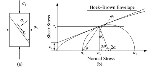
The parameter φ_i in Equations (14)(14) $$\frac{{\sigma }_{\mathrm{n}}}{{\sigma }_{\text{ci}}}=\frac{1}{m_{\mathrm{b}}}{\left(\frac{2}{m_{\mathrm{b}}a}\right)}^{\frac{1}{a-1}}{\left(\frac{\hspace{0.17em}\text{sin}\hspace{0.17em}{\varphi }_i}{1-\hspace{0.17em}\text{sin}\hspace{0.17em}{\varphi }_i}\right)}^{\frac{1}{a-1}}\left(\frac{\hspace{0.17em}\text{sin}\hspace{0.17em}{\varphi }_i}{a}+1\right)-\frac{s}{m_{\mathrm{b}}}$$(14) and (15)(15) $$\frac{{\tau }_{\mathrm{s}}}{{\sigma }_{\text{ci}}}=\left(\frac{\hspace{0.17em}\text{cos}\hspace{0.17em}{\varphi }_i}{2}\right){\left(\frac{2}{m_{\mathrm{b}}a}\right)}^{\frac{a}{a-1}}{\left(\frac{\hspace{0.17em}\text{sin}\hspace{0.17em}{\varphi }_i}{1-\hspace{0.17em}\text{sin}\hspace{0.17em}{\varphi }_i}\right)}^{\frac{a}{a-1}}$$(15) is shown in Figure 1. When the normal stress σ_n is known, sinφ_i can be easily calculated by the Newton iteration formula. Substituting the calculated sinφ_i into Equation (15)(15) $$\frac{{\tau }_{\mathrm{s}}}{{\sigma }_{\text{ci}}}=\left(\frac{\hspace{0.17em}\text{cos}\hspace{0.17em}{\varphi }_i}{2}\right){\left(\frac{2}{m_{\mathrm{b}}a}\right)}^{\frac{a}{a-1}}{\left(\frac{\hspace{0.17em}\text{sin}\hspace{0.17em}{\varphi }_i}{1-\hspace{0.17em}\text{sin}\hspace{0.17em}{\varphi }_i}\right)}^{\frac{a}{a-1}}$$(15) , then the shear stress τ_s corresponding to the normal stress σ_n can also be obtained.

Figure 1. Stress state of micro-unit at failure (a) and relationships between the Mohr stress circle and Hoek–Brown envelope in the τ – σ_n plane.

When fitting the equivalent Mohr–Coulomb strength parameters φ′ and c′ by the Hoek–Brown empirical method, σ_n is also consistent with the five normal stresses of the in-situ shear test, that is 0.497, 0.994, 1.491, 1.988, and 2.485 MPa. The shear stress τ_s corresponding to each normal stress is calculated using Equations (14)(14) $$\frac{{\sigma }_{\mathrm{n}}}{{\sigma }_{\text{ci}}}=\frac{1}{m_{\mathrm{b}}}{\left(\frac{2}{m_{\mathrm{b}}a}\right)}^{\frac{1}{a-1}}{\left(\frac{\hspace{0.17em}\text{sin}\hspace{0.17em}{\varphi }_i}{1-\hspace{0.17em}\text{sin}\hspace{0.17em}{\varphi }_i}\right)}^{\frac{1}{a-1}}\left(\frac{\hspace{0.17em}\text{sin}\hspace{0.17em}{\varphi }_i}{a}+1\right)-\frac{s}{m_{\mathrm{b}}}$$(14) and (15)(15) $$\frac{{\tau }_{\mathrm{s}}}{{\sigma }_{\text{ci}}}=\left(\frac{\hspace{0.17em}\text{cos}\hspace{0.17em}{\varphi }_i}{2}\right){\left(\frac{2}{m_{\mathrm{b}}a}\right)}^{\frac{a}{a-1}}{\left(\frac{\hspace{0.17em}\text{sin}\hspace{0.17em}{\varphi }_i}{1-\hspace{0.17em}\text{sin}\hspace{0.17em}{\varphi }_i}\right)}^{\frac{a}{a-1}}$$(15) . After obtaining the five normal-shear stress points, they can be plotted as shown in Figure 2, and the equivalent Mohr–Coulomb strength parameters φ′ and c′ can be obtained by the least square method.

Figure 2. Relationships between the normal and the shear stresses for the Hoek–Brown and Mohr–Coulomb criteria.

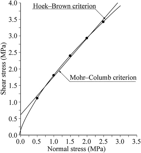
Comparing the test values of φ′ and c′ with the estimated values based on the Hoek–Brown criterion, they have a very small difference. Obviously, it is feasible to use the integrity coefficient suggested in this study to assess the disturbance factor. In particular, the basic principle of the sonic or seismic wave testing is simple, the apparatus is cheap and easy to carry, and the error owing to subjectivity is avoided.

However, if the value of D is selected according to the guidelines suggested by Hoek et al. (2002), the test values and the estimated values based on empirical formula will have a significant difference. Here, we analyze only φ′ and c′ in Table 2. The in-situ shear tests are carried out in the exploration adit, which has a diameter of ∼2 m and suffers only very weak blasting damage and stress relaxation. According to the guidelines suggested by Hoek et al. (2002), the disturbance factor D should be zero. If the same values of GSI, σ_ci, and m_i are still selected and the fitting method is the same as in the above-mentioned method, then φ′ is equal to 59.09° and c′ is equal to 0.981 MPa. Obviously, the values of φ′ and c′ calculated by the same empirical method are significantly larger than those tested in the exploration adit.

The above analysis indicates that it is feasible to assess the mechanical parameters of a rock mass with the Hoek–Brown empirical formulas after determining the values of GSI, σ_ci, D, and m_i. However, as the basic parameters of the Hoek–Brown empirical formulas are usually variable and uncertain, the estimated mechanical parameters of rock mass with the Hoek–Brown empirical formulas are also variable and uncertain. If the basic parameters of the Hoek–Brown empirical formulas are considered to be deterministic, limitations will exist in the stability assessment of a rock mass. Conversely, if their probability distributions are considered, the probability of failure and risk level can be comprehensively evaluated through a reliability analysis. Next, we will analyze the performance function in which the basic variables of the Hoek–Brown empirical formulas are contained.

3. Performance function and reliability analysis

3.1. Performance function

For the micro-unit shown in Figure 3(a), the major and minor principal stresses are denoted as σ_e1 and σ_e3, respectively, and the angle between an arbitrary section and the plane on which the minor principal stress acts is denoted as β. The Hoek–Brown shear failure envelope shown in Figure 3(b) may be obtained using Equations (14)(14) $$\frac{{\sigma }_{\mathrm{n}}}{{\sigma }_{\text{ci}}}=\frac{1}{m_{\mathrm{b}}}{\left(\frac{2}{m_{\mathrm{b}}a}\right)}^{\frac{1}{a-1}}{\left(\frac{\hspace{0.17em}\text{sin}\hspace{0.17em}{\varphi }_i}{1-\hspace{0.17em}\text{sin}\hspace{0.17em}{\varphi }_i}\right)}^{\frac{1}{a-1}}\left(\frac{\hspace{0.17em}\text{sin}\hspace{0.17em}{\varphi }_i}{a}+1\right)-\frac{s}{m_{\mathrm{b}}}$$(14) and (15)(15) $$\frac{{\tau }_{\mathrm{s}}}{{\sigma }_{\text{ci}}}=\left(\frac{\hspace{0.17em}\text{cos}\hspace{0.17em}{\varphi }_i}{2}\right){\left(\frac{2}{m_{\mathrm{b}}a}\right)}^{\frac{a}{a-1}}{\left(\frac{\hspace{0.17em}\text{sin}\hspace{0.17em}{\varphi }_i}{1-\hspace{0.17em}\text{sin}\hspace{0.17em}{\varphi }_i}\right)}^{\frac{a}{a-1}}$$(15) . Then, the factor of safety F_s of an arbitrary section of the micro-unit may be defined as the ratio of shear resistance force T_s to shear force T and is given by (16) $$F_{\mathrm{s}}=\frac{T_{\mathrm{s}}}{T}=\frac{{\tau }_{\mathrm{s}}\times \mathrm{d}S}{\tau \times \mathrm{d}S}=\frac{{\tau }_{\mathrm{s}}}{\tau }$$(16) where F_s is factor of safety, T_s is shear resistance force, T is shear force, τ_s is shear resistance, τ is shear mobilized, and dS is the area of an arbitrary section of the micro-unit.

Figure 3. Stress state of micro-unit (a) and definition the factor of safety on an arbitrary section (b).

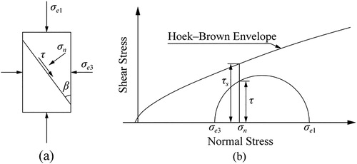
The stress circle equation shown in Figure 3(b) is written as (17) $${\left({\sigma }_{\mathrm{n}}-\frac{{\sigma }_{e1}+{\sigma }_{e3}}{2}\right)}^2+{\tau }^2={\left(\frac{{\sigma }_{e1}-{\sigma }_{e3}}{2}\right)}^2$$(17)

Substituting the shear stress τ of Equation (17)(17) $${\left({\sigma }_{\mathrm{n}}-\frac{{\sigma }_{e1}+{\sigma }_{e3}}{2}\right)}^2+{\tau }^2={\left(\frac{{\sigma }_{e1}-{\sigma }_{e3}}{2}\right)}^2$$(17) into Equation (16)(16) $$F_{\mathrm{s}}=\frac{T_{\mathrm{s}}}{T}=\frac{{\tau }_{\mathrm{s}}\times \mathrm{d}S}{\tau \times \mathrm{d}S}=\frac{{\tau }_{\mathrm{s}}}{\tau }$$(16) , then Equation (16)(16) $$F_{\mathrm{s}}=\frac{T_{\mathrm{s}}}{T}=\frac{{\tau }_{\mathrm{s}}\times \mathrm{d}S}{\tau \times \mathrm{d}S}=\frac{{\tau }_{\mathrm{s}}}{\tau }$$(16) is rewritten as (18) $$F_{\mathrm{s}}=\frac{{\tau }_{\mathrm{s}}}{\sqrt{{\left(\frac{{\sigma }_{e1}-{\sigma }_{e3}}{2}\right)}^2-{\left({\sigma }_{\mathrm{n}}-\frac{{\sigma }_{e1}+{\sigma }_{e3}}{2}\right)}^2}}$$(18)

Obviously, the minimums of F_s and $F_{\mathrm{s}}^2$ are obtained at the same point. Therefore, we solve the minimum of $F_{\mathrm{s}}^2$ in Equation (19)(19) $$F_{\mathrm{s}}^2=\frac{{\tau }_{\mathrm{s}}^2}{{\left(\frac{{\sigma }_{e1}-{\sigma }_{e3}}{2}\right)}^2-{\left({\sigma }_{\mathrm{n}}-\frac{{\sigma }_{e1}+{\sigma }_{e3}}{2}\right)}^2}$$(19) first. (19) $$F_{\mathrm{s}}^2=\frac{{\tau }_{\mathrm{s}}^2}{{\left(\frac{{\sigma }_{e1}-{\sigma }_{e3}}{2}\right)}^2-{\left({\sigma }_{\mathrm{n}}-\frac{{\sigma }_{e1}+{\sigma }_{e3}}{2}\right)}^2}$$(19)

Substituting Equations (14)(14) $$\frac{{\sigma }_{\mathrm{n}}}{{\sigma }_{\text{ci}}}=\frac{1}{m_{\mathrm{b}}}{\left(\frac{2}{m_{\mathrm{b}}a}\right)}^{\frac{1}{a-1}}{\left(\frac{\hspace{0.17em}\text{sin}\hspace{0.17em}{\varphi }_i}{1-\hspace{0.17em}\text{sin}\hspace{0.17em}{\varphi }_i}\right)}^{\frac{1}{a-1}}\left(\frac{\hspace{0.17em}\text{sin}\hspace{0.17em}{\varphi }_i}{a}+1\right)-\frac{s}{m_{\mathrm{b}}}$$(14) and (15)(15) $$\frac{{\tau }_{\mathrm{s}}}{{\sigma }_{\text{ci}}}=\left(\frac{\hspace{0.17em}\text{cos}\hspace{0.17em}{\varphi }_i}{2}\right){\left(\frac{2}{m_{\mathrm{b}}a}\right)}^{\frac{a}{a-1}}{\left(\frac{\hspace{0.17em}\text{sin}\hspace{0.17em}{\varphi }_i}{1-\hspace{0.17em}\text{sin}\hspace{0.17em}{\varphi }_i}\right)}^{\frac{a}{a-1}}$$(15) into Equation (19)(19) $$F_{\mathrm{s}}^2=\frac{{\tau }_{\mathrm{s}}^2}{{\left(\frac{{\sigma }_{e1}-{\sigma }_{e3}}{2}\right)}^2-{\left({\sigma }_{\mathrm{n}}-\frac{{\sigma }_{e1}+{\sigma }_{e3}}{2}\right)}^2}$$(19) and setting $\text{sin}\hspace{0.17em}{\varphi }_i=x$, then (20) $$F_{\mathrm{s}}^2=\frac{\frac{{\sigma }_{\text{ci}}^2}{4}{\left(\frac{2}{m_{\mathrm{b}}a}\right)}^{\frac{2a}{a-1}}(1-x^2){\left(\frac{x}{1-x}\right)}^{\frac{2a}{a-1}}}{{\left(\frac{{\sigma }_{e1}-{\sigma }_{e3}}{2}\right)}^2-{\left[\left(\frac{{\sigma }_{\text{ci}}}{m_{\mathrm{b}}}\right){\left(\frac{2}{m_{\mathrm{b}}a}\right)}^{\frac{1}{a-1}}{\left(\frac{x}{1-x}\right)}^{\frac{1}{a-1}}\left(\frac{x}{a}+1\right)-\frac{{\sigma }_{\text{ci}}s}{m_{\mathrm{b}}}-\frac{{\sigma }_{e1}+{\sigma }_{e3}}{2}\right]}^2}$$(20)

For a Hoek–Brown rock mass, because φ_i is >0 and <90°, x is >0 and <1.

As $\frac{{\sigma }_{\text{ci}}^2}{4}{\left(\frac{2}{m_{\mathrm{b}}a}\right)}^{\frac{2a}{a-1}}$ is a constant in Equation (20)(20) $$F_{\mathrm{s}}^2=\frac{\frac{{\sigma }_{\text{ci}}^2}{4}{\left(\frac{2}{m_{\mathrm{b}}a}\right)}^{\frac{2a}{a-1}}(1-x^2){\left(\frac{x}{1-x}\right)}^{\frac{2a}{a-1}}}{{\left(\frac{{\sigma }_{e1}-{\sigma }_{e3}}{2}\right)}^2-{\left[\left(\frac{{\sigma }_{\text{ci}}}{m_{\mathrm{b}}}\right){\left(\frac{2}{m_{\mathrm{b}}a}\right)}^{\frac{1}{a-1}}{\left(\frac{x}{1-x}\right)}^{\frac{1}{a-1}}\left(\frac{x}{a}+1\right)-\frac{{\sigma }_{\text{ci}}s}{m_{\mathrm{b}}}-\frac{{\sigma }_{e1}+{\sigma }_{e3}}{2}\right]}^2}$$(20) , solving the minimum of $F_{\mathrm{s}}^2$ is changed to solving the minimum of A in Equation (21)(21) $$A=\frac{(1-x^2){\left(\frac{x}{1-x}\right)}^{\frac{2a}{a-1}}}{{\left(\frac{{\sigma }_{e1}-{\sigma }_{e3}}{2}\right)}^2-{\left[\frac{{\sigma }_{\text{ci}}}{m_{\mathrm{b}}}{\left(\frac{2}{m_{\mathrm{b}}a}\right)}^{\frac{1}{a-1}}{\left(\frac{x}{1-x}\right)}^{\frac{1}{a-1}}\left(\frac{x}{a}+1\right)-\frac{{\sigma }_{\text{ci}}s}{m_{\mathrm{b}}}-\frac{{\sigma }_{e1}+{\sigma }_{e3}}{2}\right]}^2}$$(21) . (21) $$A=\frac{(1-x^2){\left(\frac{x}{1-x}\right)}^{\frac{2a}{a-1}}}{{\left(\frac{{\sigma }_{e1}-{\sigma }_{e3}}{2}\right)}^2-{\left[\frac{{\sigma }_{\text{ci}}}{m_{\mathrm{b}}}{\left(\frac{2}{m_{\mathrm{b}}a}\right)}^{\frac{1}{a-1}}{\left(\frac{x}{1-x}\right)}^{\frac{1}{a-1}}\left(\frac{x}{a}+1\right)-\frac{{\sigma }_{\text{ci}}s}{m_{\mathrm{b}}}-\frac{{\sigma }_{e1}+{\sigma }_{e3}}{2}\right]}^2}$$(21)

Differentiating Equation (21)(21) $$A=\frac{(1-x^2){\left(\frac{x}{1-x}\right)}^{\frac{2a}{a-1}}}{{\left(\frac{{\sigma }_{e1}-{\sigma }_{e3}}{2}\right)}^2-{\left[\frac{{\sigma }_{\text{ci}}}{m_{\mathrm{b}}}{\left(\frac{2}{m_{\mathrm{b}}a}\right)}^{\frac{1}{a-1}}{\left(\frac{x}{1-x}\right)}^{\frac{1}{a-1}}\left(\frac{x}{a}+1\right)-\frac{{\sigma }_{\text{ci}}s}{m_{\mathrm{b}}}-\frac{{\sigma }_{e1}+{\sigma }_{e3}}{2}\right]}^2}$$(21) with respect to x, and setting the first-order derivative of A as zero, then (22) $$pqr-w\left[{\left(\frac{{\sigma }_{e1}-{\sigma }_{e3}}{2}\right)}^2-p^2\right]=0$$(22) where $p=q\left(\frac{x}{a}+1\right)-\frac{{\sigma }_{\text{ci}}s}{m_{\mathrm{b}}}-\frac{{\sigma }_{e1}+{\sigma }_{e3}}{2}$; $q=\left(\frac{{\sigma }_{\text{ci}}}{m_{\mathrm{b}}}\right){\left(\frac{2}{m_{\mathrm{b}}a}\right)}^{\frac{1}{a-1}}{\left(\frac{x}{1-x}\right)}^{\frac{1}{a-1}}$; $r=(1-a)x^3+x^2+2ax+a$; $w=(a^2-a)x^2-a^{2}x-a^2$.

Setting the left-hand side of Equation (22)(22) $$pqr-w\left[{\left(\frac{{\sigma }_{e1}-{\sigma }_{e3}}{2}\right)}^2-p^2\right]=0$$(22) as f(x), and adopting the Newton iteration formula, (23) $$x_{k+1}=x_k-\frac{f\left(x_k\right)}{f^{\prime }\left(x_k\right)}(k=0,1,\dots )$$(23)

That is, (24) $$x_{k+1}=x_k-\frac{pqr-w\left({\left(\frac{{\sigma }_{e1}-{\sigma }_{e3}}{2}\right)}^2-p^2\right)}{p^{\prime }qr+2wp{p}^{\prime }+pq\left(u-\frac{r}{(1-a)(x-x^2)}\right)-v\left({\left(\frac{{\sigma }_{e1}-{\sigma }_{e3}}{2}\right)}^2-p^2\right)}(k=0,1,\dots )$$(24) where $p^{\prime }=q\times \frac{(1-a)x^2+ax+a}{(a^2-a)(x-x^2)}$; $u=3(1-a)x^2+2x+2a$; $v=2a(a-1)x-a^2$.

After x is solved through the above Newton iteration formula, σ_n and τ_s are obtained by substituting x into Equations (14)(14) $$\frac{{\sigma }_{\mathrm{n}}}{{\sigma }_{\text{ci}}}=\frac{1}{m_{\mathrm{b}}}{\left(\frac{2}{m_{\mathrm{b}}a}\right)}^{\frac{1}{a-1}}{\left(\frac{\hspace{0.17em}\text{sin}\hspace{0.17em}{\varphi }_i}{1-\hspace{0.17em}\text{sin}\hspace{0.17em}{\varphi }_i}\right)}^{\frac{1}{a-1}}\left(\frac{\hspace{0.17em}\text{sin}\hspace{0.17em}{\varphi }_i}{a}+1\right)-\frac{s}{m_{\mathrm{b}}}$$(14) and (15)(15) $$\frac{{\tau }_{\mathrm{s}}}{{\sigma }_{\text{ci}}}=\left(\frac{\hspace{0.17em}\text{cos}\hspace{0.17em}{\varphi }_i}{2}\right){\left(\frac{2}{m_{\mathrm{b}}a}\right)}^{\frac{a}{a-1}}{\left(\frac{\hspace{0.17em}\text{sin}\hspace{0.17em}{\varphi }_i}{1-\hspace{0.17em}\text{sin}\hspace{0.17em}{\varphi }_i}\right)}^{\frac{a}{a-1}}$$(15) , respectively. Then, the minimum of the factor of safety, denoted as F_smin, is solved by substituting σ_n and τ_s into Equation (18)(18) $$F_{\mathrm{s}}=\frac{{\tau }_{\mathrm{s}}}{\sqrt{{\left(\frac{{\sigma }_{e1}-{\sigma }_{e3}}{2}\right)}^2-{\left({\sigma }_{\mathrm{n}}-\frac{{\sigma }_{e1}+{\sigma }_{e3}}{2}\right)}^2}}$$(18) . Obviously, for a Hoek–Brown rock mass, F_smin = 1 means limit equilibrium, F_smin > 1 shows stability, and F_smin < 1 represents failure. Then, a performance function based on the factor of safety is defined as the following equation: (25) $$Z=F_{\mathrm{s}\min }-1.0$$(25)

As shown in Figure 3, when the minor principal stress σ_e3 is negative and less than the tensile strength, the above-mentioned factor of safety F_smin is equals to zero. To avoid the mathematical oddness that the dividend number may be zero in the following reliability calculation, the factor of safety should adopt the value calculated by Equation (26)(26) $$F_{\text{smin}}=\frac{{\sigma }_t}{{\sigma }_{e3}}$$(26) : (26) $$F_{\text{smin}}=\frac{{\sigma }_t}{{\sigma }_{e3}}$$(26) where σ_t is the tensile strength and can be calculated by Equation (5)(5) $${\sigma }_{\mathrm{t}}=-\frac{s{\sigma }_{\text{ci}}}{m_{\mathrm{b}}}$$(5) .

According to the finite element theory, we know that the elastic stresses can be directly calculated if the modulus of deformation E_m, Poisson’s ratio μ, and unit weight γ of the rock mass are known. It should be noted that E_m can be obtained by Equation (10)(10) $$\{\begin{array}{ll}{E}_{\mathrm{m}}=\left(1-\frac{D}{2}\right)\sqrt{\frac{{\sigma }_{\text{ci}}}{100}}\times {10}^{\frac{\text{GSI}-10}{40}}& ({\sigma }_{\text{ci}}\le 100\text{MPa})\\ E_{\mathrm{m}}=\left(1-\frac{D}{2}\right)\times {10}^{\frac{\text{GSI}-10}{40}}& ({\sigma }_{\text{ci}}>100\text{MPa})\end{array}$$(10) . The factor of safety F_smin is calculated based on the Hoek–Brown criterion and also related to the rock mass stresses. Therefore, Equation (25)(25) $$Z=F_{\mathrm{s}\min }-1.0$$(25) can be rewritten as: (27) $$Z=F_{\text{sm}in}(\text{GSI},D,{\sigma }_{\text{ci}},m_{\mathrm{i}},\mu ,\gamma )-1.0$$(27) where GSI is the geological strength index, D is the disturbance factor, σ_ci is the uniaxial compressive strength of intact rock, m_i is the material parameter of intact rock, μ is the Poisson’s ratio, and γ is the natural unit weight of rock.

When the mean and standard deviation of the basic variables in Equation (27)(27) $$Z=F_{\text{sm}in}(\text{GSI},D,{\sigma }_{\text{ci}},m_{\mathrm{i}},\mu ,\gamma )-1.0$$(27) are determined, the reliability index or failure probability in any element of the rock mass can be obtained with the reliability analysis methods. According to the actual basic data, such as laboratory test results and geology exploration data, the mean and standard deviation of the basic variables can be acquired by statistical analysis methods. When laboratory tests are not possible and the preliminary geology explorations are poor, their respective mean and standard deviation can also be estimated using “three sigma rule” (Dai and Wang 1992).

Theoretically, the probability that a random variable conforming to a normal distribution lies between ±3σ is 99.73%, and σ is the standard deviation. We know that the probabilistic values of the basic variables in Equation (27)(27) $$Z=F_{\text{sm}in}(\text{GSI},D,{\sigma }_{\text{ci}},m_{\mathrm{i}},\mu ,\gamma )-1.0$$(27) will never touch –∞ or +∞. For practical purposes, it is feasible to assume that the extremely possible interval of each basic variable lies between ±3σ. When the extremely possible interval of each basic variable in Equation (27)(27) $$Z=F_{\text{sm}in}(\text{GSI},D,{\sigma }_{\text{ci}},m_{\mathrm{i}},\mu ,\gamma )-1.0$$(27) is estimated, the corresponding standard deviation can be considered as the difference between the highest and the lowest values, divided by 6, and the corresponding mean can be considered as the median value between them. As the basic variables in Equation (27)(27) $$Z=F_{\text{sm}in}(\text{GSI},D,{\sigma }_{\text{ci}},m_{\mathrm{i}},\mu ,\gamma )-1.0$$(27) usually obey a normal distribution, their respective mean and standard deviation can be estimated using the “three sigma rule”. However, for preliminary field investigations or “low budget” projects, it is prudent to estimate a larger interval for each basic variable in Equation (27)(27) $$Z=F_{\text{sm}in}(\text{GSI},D,{\sigma }_{\text{ci}},m_{\mathrm{i}},\mu ,\gamma )-1.0$$(27) .

3.2. Reliability analysis methods

There are many methods to assess the stability reliability of a rock mass, such as the Taylor series, Rosenblueth point estimate, and Monte Carlo methods.

The Taylor series method is based on the Taylor series expansion of a performance function about some point (U.S. Army Corps of Engineers 1997). As only the first-order (linear) terms of the Taylor series expansion are retained and only the first two moments (mean and standard deviation) are used, this method is often termed a first-order second-moment method. The method is exact for linear performance functions. However, the neglect of higher order terms will result in significant errors for non-linear functions.

An alternative method to estimate the moments of a performance function based on the moments of the random variables is the Rosenblueth point estimate method, proposed by Rosenblueth (1981) and summarized by Harr (1987). For a symmetrically distributed random variable, the point estimates are taken at the mean plus and minus one standard deviation. This method can be used to calculate the first two moments (mean and standard deviation) of the performance function when the probability distributions of the variables are not known. However, the number of combinations increases with the number of variables.

The Monte Carlo method is based on the law of large numbers in mathematics. Theoretically, the more trial runs are used in an analysis, the more accurate the solution will be. However, how many trials are required in a probabilistic analysis? According to the studies by Harr (1987), the number of Monte Carlo trials increases geometrically with the level of confidence and the number of variables, and the empirical equation is given by (28) $$N={\left(\frac{K_{a/2}^2}{4{(1-a)}^2}\right)}^n$$(28) where N is the number of Monte Carlo trials; a is the desired level of confidence (0–100%), expressed in decimal form; K_a/2 is the normal standard deviate corresponding to the level of confidence, expressed as $K_{a/2}={\Phi }^{-1}(1-a/2)=1-\Phi (1-a/2)$, and which can be obtained by inquiring the normal distribution table; and n is the number of random variables.

3.3. Calculation procedures

The mean and standard deviation of a performance function can be obtained with any one of the above-mentioned methods. Then, the reliability index or probability of failure can be calculated with the calculated mean and standard deviation.

Clearly, the performance function in Equation (27)(27) $$Z=F_{\text{sm}in}(\text{GSI},D,{\sigma }_{\text{ci}},m_{\mathrm{i}},\mu ,\gamma )-1.0$$(27) is non-linear. As mentioned above, direct use of the Taylor series method is not appropriate owing to the neglect of higher order terms. Also, it needs a great number of trials in the Monte Carlo method to guarantee the high level of confidence. Thus, we choose the Rosenblueth point estimation method to estimate the mean and standard deviation of the factor of safety of the element. Next, the process calculating the reliability index of the Hoek–Brown rock mass stability with the combination of the Rosenblueth point estimate and finite element methods will be described in detail.

First, it is assumed that the basic variables in Equation (27)(27) $$Z=F_{\text{sm}in}(\text{GSI},D,{\sigma }_{\text{ci}},m_{\mathrm{i}},\mu ,\gamma )-1.0$$(27) are independent of each other. Furthermore, the basic variables in Equation (27)(27) $$Z=F_{\text{sm}in}(\text{GSI},D,{\sigma }_{\text{ci}},m_{\mathrm{i}},\mu ,\gamma )-1.0$$(27) usually abide by the normal distribution. For the Rosenblueth point estimate method, the two point estimates of each variable are taken at the mean plus or minus one standard deviation. As the number of random variables n is 6, all possible combinations of point estimates are 2ⁿ = 2⁶ = 64, correspondingly producing 64 solutions of the safety factor. To avoid repetition and confusion, all combinations can be carried out by a computer programme. In this study, the programme code for the point estimate combinations of variables is written in Fortran language (Table 3).

Table 3. Fortran code for the point estimate combinations of variables in the performance function.

… Double Dimension GSI(2), SIGMAC(2), D(2), MI(2), POISSON(2), GARMA(2) ! GSI(1)=GSI+, GSI(2)=GSI-; SIGMAC(1)=σci+, SIGMAC(2)=σci–; D(2)=D+, D(2)=D– ! MI(1)=Mi+, MI(2)=Mi–; POISSON(1)=μ+, POISSON(2)=μ–; GARMA(2)=γ+, GARMA(2)=γ– DO 10 i = 1,2,1 DO 10 j = 1,2,1 DO 10 k = 1,2,1 DO 10 l = 1,2,1 DO 10 m = 1,2,1 DO 10 n = 1,2,1 ! GSI(i), SIGMAC(j), D(k), MI(l), POISSON(m), GARMA(n) ! A combination used to calculate rock mass mechanical parameter value with H-B formulas … 10 CONTINUE …

For each combination of the basic variables in Equation (27)(27) $$Z=F_{\text{sm}in}(\text{GSI},D,{\sigma }_{\text{ci}},m_{\mathrm{i}},\mu ,\gamma )-1.0$$(27) , after the elastic stresses of the element in a numerical model are calculated by the finite element method, the factor of safety of the element is solved using the method introduced in this study. As the number of all combinations is 64, the number of factors of safety of the element is also 64. The basic variables in Equation (27)(27) $$Z=F_{\text{sm}in}(\text{GSI},D,{\sigma }_{\text{ci}},m_{\mathrm{i}},\mu ,\gamma )-1.0$$(27) have been assumed to be independent of each other. Thus, the probability of each combination is 1/64. Then the first-moment M₁ or expected value E[F] or mean μ_F of point estimates can be calculated by (29) $$M_1=E\left[F\right]={\mu }_{\mathrm{F}}\approx \frac{1}{2^6}\sum _{j=1}^{2^6}\left(F_j\right)$$(29)

The second-moment M₂ or population variance ${\sigma }_{\mathrm{F}}^2$ of the point estimates can be calculated by (30) $$M_2={\sigma }_{\mathrm{F}}^2\approx \frac{1}{2^6}\sum _{j=1}^{2^6}\left(F_j^2\right)-{\mu }_{\mathrm{F}}^2$$(30)

According to the studies by Wolff (1996), it is reasonable to assume that the slope factor of safety will be adequately represented by a normal distribution (Wolff 1996). However, Duncan believed that the distribution of factors of safety approximately conforms to a lognormal distribution (Duncan 2000).

When the probability distribution of factors of safety of the element in a numerical model is assumed to be normal, the reliability index should be calculated by Equation (31)(31) $${\beta }_{\mathrm{N}}=\frac{({\mu }_{\mathrm{F}}-1)}{{\sigma }_{\mathrm{F}}}$$(31) (Wolff 1996). (31) $${\beta }_{\mathrm{N}}=\frac{({\mu }_{\mathrm{F}}-1)}{{\sigma }_{\mathrm{F}}}$$(31) where β_N is the reliability index, μ_F is the mean, and σ_F is the standard deviation.

When the probability distribution is assumed to be lognormal, the reliability index should be calculated by Equation (32)(32) $${\beta }_{\hspace{0.17em}\text{LN}\hspace{0.17em}}=\frac{\hspace{0.17em}\text{ln}\hspace{0.17em}\left(\frac{{\mu }_{\mathrm{F}}}{1+V_{\mathrm{F}}^2}\right)}{\sqrt{\hspace{0.17em}\text{ln}\hspace{0.17em}\left(1+V_{\mathrm{F}}^2\right)}}$$(32) (Duncan 2000) (32) $${\beta }_{\hspace{0.17em}\text{LN}\hspace{0.17em}}=\frac{\hspace{0.17em}\text{ln}\hspace{0.17em}\left(\frac{{\mu }_{\mathrm{F}}}{1+V_{\mathrm{F}}^2}\right)}{\sqrt{\hspace{0.17em}\text{ln}\hspace{0.17em}\left(1+V_{\mathrm{F}}^2\right)}}$$(32) where β_LN is the reliability index and V_F is the coefficient of variation, which is equals to the ratio of the standard deviation to the mean, that is $V_{\mathrm{F}}={\sigma }_{\mathrm{F}}/{\mu }_{\mathrm{F}}$.

Then the probability of failure can be calculated by (33) $$P_{\mathrm{f}}=1-\Phi (\beta )$$(33) where Φ() is the standard normal distribution function.

Theoretically, if a numerical model contains two and more Hoek–Brown rock masses, the Rosenblueth point estimation method can also be used. However, if GSI, σ_ci, D, m_i, μ, and γ of each Hoek–Brown rock mass are simultaneously considered as variables, the number of combinations will increase significantly with the number of materials. For example, if n = 5, then 2⁶ⁿ = 2^{6 × 5} = 2³⁰ = 1,073,741,824. Obviously, the magnitude of the calculation is very great. According to the authors’ experience, to obtain the reliability index or the probability of failure of each Hoek–Brown rock mass, GSI, σ_ci, D, m_i, μ, and γ of a certain Hoek–Brown rock mass are considered as variables, and those of the others are considered as constants and taken only at their respective mean. Then, the number of combinations is only 64 × n, and the number of calculations is greatly reduced.

4. Analysis of a cutting slope

4.1. Geology conditions

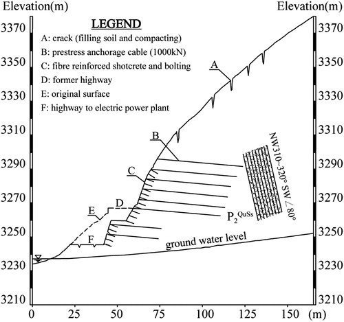
An example of a cutting slope in the Laohuzui Hydropower Station in Tibet of China will be used to illustrate the reliability analysis process using the methods introduced in this study. The Laohuzui Hydropower Station is located on the Bahe River, a branch of the Yalu Tsangpo River in Tibet. The Himalaya Mountains are at the southwest side of the hydropower station. The heights of the natural valley slopes near the hydropower station are over 500 m. The lithologies in the cutting slope studied in this study are metamorphic quartz sandstone and sandy slate, and the sandy slate accounts for ∼9.4% of the total thickness of the formation. The bedding surface of the rock is nearly vertical. Because of earthquake shaking, tectonic uplift, rapid stream erosion, steepening of valley sides, and removal of the lateral support by the glaciers now melted near the Himalaya Mountains, rock joints are widely distributed in the rock masses of natural slopes. Furthermore, toppling failures occur near the surfaces of natural slopes.

The cutting slope example (Figure 4) is located near the outlets of the diversion and spillway tunnels. Geological investigations show that the slope has suffered intensive unloading activities in the geologic evolution process. As rock joints are widely distributed in the cutting slope, it is reasonable to assume the numerical model as homogeneous. The blast damage and stress relaxation owing to excavation have significant influences on the slope stability. During excavation, a series of cracks occur at the slope shoulder of the former highway slope. Furthermore, small rockfall events occur frequently (Figure 4). To guarantee the construction safety and long-time stability of the cutting slope, the reinforcement measures mainly include two steps: (1) applying pre-stressed anchorage bolts to the former highway slope; (2) cutting the rock masses below the former highway according to the design plan (Figure 5). The above-mentioned method is adopted to assess its stability reliability and demonstrate the length of the anchorage cable. The typical section is shown in Figure 5.

Figure 4. Photograph near the outlets of the diversion and spillway tunnels and failure features.

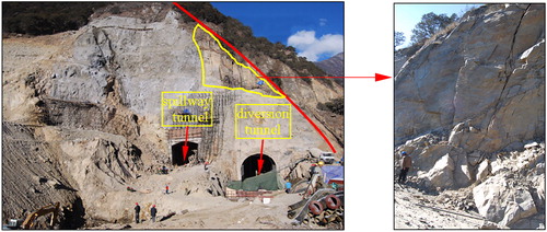
Figure 5. Typical section of the cutting slope.

According to the test results and geological investigations, the mean and standard deviation of each variable in Equation (27)(27) $$Z=F_{\text{sm}in}(\text{GSI},D,{\sigma }_{\text{ci}},m_{\mathrm{i}},\mu ,\gamma )-1.0$$(27) is obtained. The geological strength index is GSI =40.0 ± 2.5, disturbance factor is D = 0.859 ± 0.076, uniaxial compressive strength of intact rock is σ_ci = 124.88 ± 18.69 MPa, material parameter of intact rock is m_i = 19.04 ± 3.02, Poisson’s ratio is μ = 0.28 ± 0.02, and natural unit weight of rock is γ = 2.69 ± 0.05 kN/m³. It should be noted that the mean and standard deviation of each variable are denoted as “mean ± standard deviation”. The two-dimensional numerical model is considered to be homogeneous, and only the gravitational stress field is taken into account. The horizontal displacements are fixed for the nodes along the left- and right-hand side boundaries, whereas both the horizontal and the vertical displacements are fixed along the bottom boundary. The factor of safety of the element in the numerical model is assumed to be normal, and the reliability index of the element is calculated by Equation (31)(31) $${\beta }_{\mathrm{N}}=\frac{({\mu }_{\mathrm{F}}-1)}{{\sigma }_{\mathrm{F}}}$$(31) .

4.2. Results

According to the methods introduced in this study, the reliability index, probability of failure, and factor of safety of the element in the numerical model are calculated, and their respective contour distributions are plotted in Figures 6–8. The factor of safety shown in Figure 8 is the mean based on the probability theory. To compare with Figure 8, the basic variables are also considered to be deterministic. Here, the basic viabilities are taken at their respective mean, and the factor of safety is also calculated and plotted in Figure 9.

Figure 6. Reliability index.

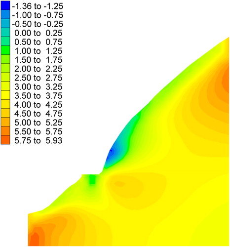
Figure 7. Probability of failure.

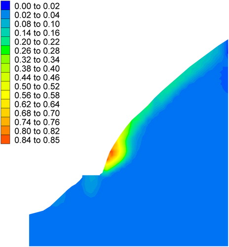
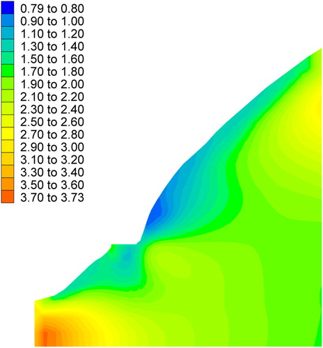
Figure 8. Mean of factor of safety based on the probability theory.

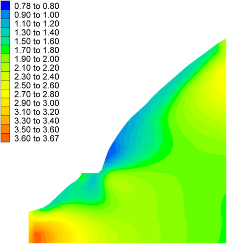
Figure 9. Factor of safety based on the deterministic analysis.

4.3. Analysis and discussion

From the analysis of the computational results, we can see that the reliability index in the toe and near the surface of the former highway slope is lower than that in other positions (Figure 6). Furthermore, the probability of failure in the toe and near the surface of the former highway slope is larger than that in other positions (Figure 7). The computational result is very consistent with the slope failure that occurred (Figure 4). Although the contour distributions of the factor of safety (Figure 9) based on the deterministic analysis is consistent with those of the factor of safety (Figure 8) based on the probability theory, the probability of failure and the risk level can be known well through the reliability analysis.

According to the Chinese Design Specification (Power Trade Criterion of P. R. China 2006), the designed grade of the cutting slope is the 5th grade. As there are few local residents and the harmfulness of the cutting slope is low, the designed probability of failure is <0.1% and the corresponding reliability index is 3.10. The computational results show that the maximum depths of potential failure to the surface above and below the former highway are ∼40 and 35 m, respectively. Therefore, the maximum anchorage depth (50 m) can meet the design requirements (Figures 6 and 7).

5. Conclusion

1. The quantitative assessment method for the disturbance factor, based on the longitudinal wave velocity measured by sonic or seismic methods, is rational and can be used to estimate the disturbance degree of a non-excavated rock mass, such as natural valley slopes. In the application of the method presented in this study, measuring sonic or seismic wave velocities and testing other physical and mechanical parameters of rock or rock mass should be carried out in the same grade rock masses with similar engineering properties.

2. The performance function, established based on the factor of safety of the element, contains the basic variables of the Hoek–Brown empirical formulas and embodies their basic features. Furthermore, it is realized that the reliability analysis of rock mass stability is implemented directly starting with the basic variables of the Hoek–Brown empirical formulas.

3. The method deriving the factor of safety of the element from the Hoek–Brown criterion is also applicable to the other non-linear strength criteria. The quantitative assessment method for the disturbance factor and the reliability assessment method based on the Hoek–Brown empirical formulas can be used in slopes, foundations, and underground caverns related to rock mass.

Acknowledgments

The authors thank Elsevier’s Webshop for editing and polishing this article. The authors also thank the anonymous reviewers for the valuable comments and time devoted to improving this article.

Disclosure statement

No potential conflict of interest was reported by the authors.

Additional information

Funding

This study was supported by The National Nature Science Foundation of China [Grant No. 41772321], the Basic Geological Survey Project of China Geological Survey [Grant No. DD20160272], and the International Cooperation Project of Sichuan Province [Grant No. 2018HH0082].

Appendix A

Derivation of Equations (14) and (15)

When a micro-unit is just in the state of critical failure, the normal and shear stresses of failure are given by (A.1) $$\{\begin{array}{l}{\sigma }_{\mathrm{n}}=\frac{{\sigma }_1+{\sigma }_3}{2}-\frac{{\sigma }_1-{\sigma }_3}{2}\text{cos}\hspace{0.17em}2\theta \\ {\tau }_{\mathrm{s}}=\frac{{\sigma }_1-{\sigma }_3}{2}\text{sin}\hspace{0.17em}2\theta \end{array}$$(A.1) where σ_n and τ_s are the normal and shear stresses of the failure plane, respectively; ${{\sigma }^{\prime }}_1$ and ${{\sigma }^{\prime }}_3$ are the major and minor effective principal stresses at failure, respectively (note that the compressive stress is taken as positive); and θ is the angle between the failure plane and the plane on which the minor principal stress acts.

As shown in Figure 1(b), Equation (A.1)(A.1) $$\{\begin{array}{l}{\sigma }_{\mathrm{n}}=\frac{{\sigma }_1+{\sigma }_3}{2}-\frac{{\sigma }_1-{\sigma }_3}{2}\text{cos}\hspace{0.17em}2\theta \\ {\tau }_{\mathrm{s}}=\frac{{\sigma }_1-{\sigma }_3}{2}\text{sin}\hspace{0.17em}2\theta \end{array}$$(A.1) is rewritten as follows (the symbol φ_i is shown in Figure 1(b)): (A.2) $$\{\begin{array}{l}{\sigma }_{\mathrm{n}}=\frac{{\sigma }_1+{\sigma }_3}{2}-\frac{{\sigma }_1-{\sigma }_3}{2}\text{sin}\hspace{0.17em}{\varphi }_i\\ {\tau }_{\mathrm{s}}=\frac{{\sigma }_1-{\sigma }_3}{2}\text{cos}\hspace{0.17em}{\varphi }_i\end{array}$$(A.2)

According to the Mohr–Coulomb criterion, $\frac{d{\sigma }_1}{d{\sigma }_3}=\frac{1+\hspace{0.17em}\text{sin}\hspace{0.17em}{\varphi }_i}{1-\hspace{0.17em}\text{sin}\hspace{0.17em}{\varphi }_i}$ can be derived, and $\text{sin}\hspace{0.17em}{\varphi }_i=\frac{d{\sigma }_1/d{\sigma }_3-1}{d{\sigma }_1/d{\sigma }_3+1}$ is obtained. According to the trigonometric functions, $\text{cos}\hspace{0.17em}{\varphi }_i=\frac{2\sqrt{d{\sigma }_1/d{\sigma }_3}}{d{\sigma }_1/d{\sigma }_3+1}$ is also obtained. Substituting them into Equation (A.2)(A.2) $$\{\begin{array}{l}{\sigma }_{\mathrm{n}}=\frac{{\sigma }_1+{\sigma }_3}{2}-\frac{{\sigma }_1-{\sigma }_3}{2}\text{sin}\hspace{0.17em}{\varphi }_i\\ {\tau }_{\mathrm{s}}=\frac{{\sigma }_1-{\sigma }_3}{2}\text{cos}\hspace{0.17em}{\varphi }_i\end{array}$$(A.2) , then (A.3) $$\{\begin{array}{l}{\sigma }_{\mathrm{n}}=\frac{{\sigma }_1-{\sigma }_3}{1+d{\sigma }_1/d{\sigma }_3}+{\sigma }_3\\ {\tau }_{\mathrm{s}}=\frac{{\sigma }_1-{\sigma }_3}{1+d{\sigma }_1/d{\sigma }_3}\sqrt{d{\sigma }_1/d{\sigma }_3}\end{array}$$(A.3) $\text{tan}\hspace{0.17em}\alpha =\frac{{\tau }_{\mathrm{s}}}{{\sigma }_{\mathrm{n}}-{\sigma }_3}$ is derived directly from Figure 1(b), and substituting it into Equation (A.3)(A.3) $$\{\begin{array}{l}{\sigma }_{\mathrm{n}}=\frac{{\sigma }_1-{\sigma }_3}{1+d{\sigma }_1/d{\sigma }_3}+{\sigma }_3\\ {\tau }_{\mathrm{s}}=\frac{{\sigma }_1-{\sigma }_3}{1+d{\sigma }_1/d{\sigma }_3}\sqrt{d{\sigma }_1/d{\sigma }_3}\end{array}$$(A.3) , then (A.4) $$\text{tan}\hspace{0.17em}\alpha =\sqrt{d{\sigma }_1/d{\sigma }_3}$$(A.4) $\text{tan}\hspace{0.17em}2\alpha =\hspace{0.17em}\text{tan}\hspace{0.17em}\left({\varphi }_i+\frac{\pi }{2}\right)=-\text{cot}{\varphi }_i$ is also derived directly from Figure 1(b). According to the trigonometric functions, $\text{tan}\hspace{0.17em}2\alpha =\frac{2\hspace{0.17em}\text{tan}\hspace{0.17em}\alpha }{1-{\hspace{0.17em}\text{tan}\hspace{0.17em}}^2\alpha }$ is obtained. Thus, Equation (A.5)(A.5) $$\text{tan}\hspace{0.17em}\alpha =\frac{1+\hspace{0.17em}\text{sin}\hspace{0.17em}{\varphi }_i}{\hspace{0.17em}\text{cos}\hspace{0.17em}{\varphi }_i}$$(A.5) is derived, (A.5) $$\text{tan}\hspace{0.17em}\alpha =\frac{1+\hspace{0.17em}\text{sin}\hspace{0.17em}{\varphi }_i}{\hspace{0.17em}\text{cos}\hspace{0.17em}{\varphi }_i}$$(A.5)

Solving simultaneously Equations (A.4)(A.4) $$\text{tan}\hspace{0.17em}\alpha =\sqrt{d{\sigma }_1/d{\sigma }_3}$$(A.4) and (A.5)(A.5) $$\text{tan}\hspace{0.17em}\alpha =\frac{1+\hspace{0.17em}\text{sin}\hspace{0.17em}{\varphi }_i}{\hspace{0.17em}\text{cos}\hspace{0.17em}{\varphi }_i}$$(A.5) , then (A.6) $$\frac{1+\hspace{0.17em}\text{sin}\hspace{0.17em}{\varphi }_i}{\hspace{0.17em}\text{cos}\hspace{0.17em}{\varphi }_i}=\sqrt{d{\sigma }_1/d{\sigma }_3}$$(A.6)

Differentiating Equation (1)(1) $${{\sigma }^{\prime }}_1={{\sigma }^{\prime }}_3+{\sigma }_{\text{ci}}{\left(m_{\mathrm{b}}\frac{{{\sigma }^{\prime }}_3}{{\sigma }_{\text{ci}}}+s\right)}^{\alpha }$$(1) with respect to σ₃, Equation (A.7) is derived, (A.7) $$\frac{d{\sigma }_1}{d{\sigma }_3}=1+m_{\mathrm{b}}a{\left(m_{\mathrm{b}}\frac{{\sigma }_3}{{\sigma }_{\text{ci}}}+s\right)}^{a-1}$$(A.7)

Equation (1)(1) $${{\sigma }^{\prime }}_1={{\sigma }^{\prime }}_3+{\sigma }_{\text{ci}}{\left(m_{\mathrm{b}}\frac{{{\sigma }^{\prime }}_3}{{\sigma }_{\text{ci}}}+s\right)}^{\alpha }$$(1) can be rewritten as (A.8) $$m_{\mathrm{b}}\frac{{\sigma }_3}{{\sigma }_{\text{ci}}}+s={\left(\frac{{\sigma }_1-{\sigma }_3}{{\sigma }_{\text{ci}}}\right)}^{\frac{1}{a}}$$(A.8)

Substituting Equation (A.8)(A.8) $$m_{\mathrm{b}}\frac{{\sigma }_3}{{\sigma }_{\text{ci}}}+s={\left(\frac{{\sigma }_1-{\sigma }_3}{{\sigma }_{\text{ci}}}\right)}^{\frac{1}{a}}$$(A.8) into Equation (A.7)(A.7) $$\frac{d{\sigma }_1}{d{\sigma }_3}=1+m_{\mathrm{b}}a{\left(m_{\mathrm{b}}\frac{{\sigma }_3}{{\sigma }_{\text{ci}}}+s\right)}^{a-1}$$(A.7) , then (A.9) $$\frac{d{\sigma }_1}{d{\sigma }_3}=1+m_{\mathrm{b}}a{\left(\frac{{\sigma }_1-{\sigma }_3}{{\sigma }_{\text{ci}}}\right)}^{\frac{a-1}{a}}$$(A.9)

Rewriting the expression of τ_s in Equation (A.3)(A.3) $$\{\begin{array}{l}{\sigma }_{\mathrm{n}}=\frac{{\sigma }_1-{\sigma }_3}{1+d{\sigma }_1/d{\sigma }_3}+{\sigma }_3\\ {\tau }_{\mathrm{s}}=\frac{{\sigma }_1-{\sigma }_3}{1+d{\sigma }_1/d{\sigma }_3}\sqrt{d{\sigma }_1/d{\sigma }_3}\end{array}$$(A.3) , then (A.10) $$\frac{{\sigma }_1-{\sigma }_3}{{\sigma }_{\text{ci}}}=\frac{{\tau }_{\mathrm{s}}\left(1+d{\sigma }_1/d{\sigma }_3\right)}{{\sigma }_{\text{ci}}\sqrt{d{\sigma }_1/d{\sigma }_3}}$$(A.10)

According to Equation (A.6)(A.6) $$\frac{1+\hspace{0.17em}\text{sin}\hspace{0.17em}{\varphi }_i}{\hspace{0.17em}\text{cos}\hspace{0.17em}{\varphi }_i}=\sqrt{d{\sigma }_1/d{\sigma }_3}$$(A.6) , $\frac{\left(1+d{\sigma }_1/d{\sigma }_3\right)}{\sqrt{d{\sigma }_1/d{\sigma }_3}}$ at the right-hand side of Equation (A.10)(A.10) $$\frac{{\sigma }_1-{\sigma }_3}{{\sigma }_{\text{ci}}}=\frac{{\tau }_{\mathrm{s}}\left(1+d{\sigma }_1/d{\sigma }_3\right)}{{\sigma }_{\text{ci}}\sqrt{d{\sigma }_1/d{\sigma }_3}}$$(A.10) is expressed as a function related to φ_i, as follows: (A.11) $$\frac{1+d{\sigma }_1/d{\sigma }_3}{\sqrt{d{\sigma }_1/d{\sigma }_3}}=\frac{1+{\left(\frac{1+\hspace{0.17em}\text{sin}\hspace{0.17em}{\varphi }_i}{\hspace{0.17em}\text{cos}\hspace{0.17em}{\varphi }_i}\right)}^2}{\frac{1+\hspace{0.17em}\text{sin}\hspace{0.17em}{\varphi }_i}{\hspace{0.17em}\text{cos}\hspace{0.17em}{\varphi }_i}}=\frac{2}{\hspace{0.17em}\text{cos}\hspace{0.17em}{\varphi }_i}$$(A.11)

Substituting Equation (A.11)(A.11) $$\frac{1+d{\sigma }_1/d{\sigma }_3}{\sqrt{d{\sigma }_1/d{\sigma }_3}}=\frac{1+{\left(\frac{1+\hspace{0.17em}\text{sin}\hspace{0.17em}{\varphi }_i}{\hspace{0.17em}\text{cos}\hspace{0.17em}{\varphi }_i}\right)}^2}{\frac{1+\hspace{0.17em}\text{sin}\hspace{0.17em}{\varphi }_i}{\hspace{0.17em}\text{cos}\hspace{0.17em}{\varphi }_i}}=\frac{2}{\hspace{0.17em}\text{cos}\hspace{0.17em}{\varphi }_i}$$(A.11) into Equation (A.10)(A.10) $$\frac{{\sigma }_1-{\sigma }_3}{{\sigma }_{\text{ci}}}=\frac{{\tau }_{\mathrm{s}}\left(1+d{\sigma }_1/d{\sigma }_3\right)}{{\sigma }_{\text{ci}}\sqrt{d{\sigma }_1/d{\sigma }_3}}$$(A.10) , and substituting Equation (A.10)(A.10) $$\frac{{\sigma }_1-{\sigma }_3}{{\sigma }_{\text{ci}}}=\frac{{\tau }_{\mathrm{s}}\left(1+d{\sigma }_1/d{\sigma }_3\right)}{{\sigma }_{\text{ci}}\sqrt{d{\sigma }_1/d{\sigma }_3}}$$(A.10) into Equation (A.9)(A.9) $$\frac{d{\sigma }_1}{d{\sigma }_3}=1+m_{\mathrm{b}}a{\left(\frac{{\sigma }_1-{\sigma }_3}{{\sigma }_{\text{ci}}}\right)}^{\frac{a-1}{a}}$$(A.9) again, then (A.12) $$\frac{d{\sigma }_1}{d{\sigma }_3}=1+m_{\mathrm{b}}a{\left(\frac{{\tau }_{\mathrm{s}}}{{\sigma }_{\text{ci}}}\times \frac{2}{\hspace{0.17em}\text{cos}\hspace{0.17em}{\varphi }_i}\right)}^{\frac{a-1}{a}}$$(A.12)

Substituting Equation (A.6)(A.6) $$\frac{1+\hspace{0.17em}\text{sin}\hspace{0.17em}{\varphi }_i}{\hspace{0.17em}\text{cos}\hspace{0.17em}{\varphi }_i}=\sqrt{d{\sigma }_1/d{\sigma }_3}$$(A.6) into Equation (A.12)(A.12) $$\frac{d{\sigma }_1}{d{\sigma }_3}=1+m_{\mathrm{b}}a{\left(\frac{{\tau }_{\mathrm{s}}}{{\sigma }_{\text{ci}}}\times \frac{2}{\hspace{0.17em}\text{cos}\hspace{0.17em}{\varphi }_i}\right)}^{\frac{a-1}{a}}$$(A.12) , then (A.13) $${\left(\frac{1+\hspace{0.17em}\text{sin}\hspace{0.17em}{\varphi }_i}{\hspace{0.17em}\text{cos}\hspace{0.17em}{\varphi }_i}\right)}^2-1=m_{\mathrm{b}}a{\left(\frac{{\tau }_{\mathrm{s}}}{{\sigma }_{\text{ci}}}\times \frac{2}{\hspace{0.17em}\text{cos}\hspace{0.17em}{\varphi }_i}\right)}^{\frac{a-1}{a}}$$(A.13)

Equation (A.13)(A.13) $${\left(\frac{1+\hspace{0.17em}\text{sin}\hspace{0.17em}{\varphi }_i}{\hspace{0.17em}\text{cos}\hspace{0.17em}{\varphi }_i}\right)}^2-1=m_{\mathrm{b}}a{\left(\frac{{\tau }_{\mathrm{s}}}{{\sigma }_{\text{ci}}}\times \frac{2}{\hspace{0.17em}\text{cos}\hspace{0.17em}{\varphi }_i}\right)}^{\frac{a-1}{a}}$$(A.13) can be rewritten as (A.14) $$\frac{{\tau }_{\mathrm{s}}}{{\sigma }_{\text{ci}}}=\left(\frac{\hspace{0.17em}\text{cos}\hspace{0.17em}{\varphi }_i}{2}\right)\times {\left(\frac{2}{m_{\mathrm{b}}a}\right)}^{\frac{a}{a-1}}\times {\left(\frac{\hspace{0.17em}\text{sin}\hspace{0.17em}{\varphi }_i}{1-\hspace{0.17em}\text{sin}\hspace{0.17em}{\varphi }_i}\right)}^{\frac{a}{a-1}}$$(A.14)

Rewriting the expression of σ_n in Equation (A.3)(A.3) $$\{\begin{array}{l}{\sigma }_{\mathrm{n}}=\frac{{\sigma }_1-{\sigma }_3}{1+d{\sigma }_1/d{\sigma }_3}+{\sigma }_3\\ {\tau }_{\mathrm{s}}=\frac{{\sigma }_1-{\sigma }_3}{1+d{\sigma }_1/d{\sigma }_3}\sqrt{d{\sigma }_1/d{\sigma }_3}\end{array}$$(A.3) , then (A.15) $${\sigma }_3={\sigma }_{\mathrm{n}}-\frac{{\tau }_{\mathrm{s}}}{\sqrt{d{\sigma }_1/d{\sigma }_3}}$$(A.15)

Equation (A.7)(A.7) $$\frac{d{\sigma }_1}{d{\sigma }_3}=1+m_{\mathrm{b}}a{\left(m_{\mathrm{b}}\frac{{\sigma }_3}{{\sigma }_{\text{ci}}}+s\right)}^{a-1}$$(A.7) can be rewritten as (A.16) $$\frac{{\sigma }_1-{\sigma }_3}{{\sigma }_{\text{ci}}}={\left(m_{\mathrm{b}}\frac{{\sigma }_3}{{\sigma }_{\text{ci}}}+s\right)}^a$$(A.16)

Substituting Equations (A.10)(A.10) $$\frac{{\sigma }_1-{\sigma }_3}{{\sigma }_{\text{ci}}}=\frac{{\tau }_{\mathrm{s}}\left(1+d{\sigma }_1/d{\sigma }_3\right)}{{\sigma }_{\text{ci}}\sqrt{d{\sigma }_1/d{\sigma }_3}}$$(A.10) and (A.15)(A.15) $${\sigma }_3={\sigma }_{\mathrm{n}}-\frac{{\tau }_{\mathrm{s}}}{\sqrt{d{\sigma }_1/d{\sigma }_3}}$$(A.15) into Equation (A.16)(A.16) $$\frac{{\sigma }_1-{\sigma }_3}{{\sigma }_{\text{ci}}}={\left(m_{\mathrm{b}}\frac{{\sigma }_3}{{\sigma }_{\text{ci}}}+s\right)}^a$$(A.16) , then (A.17) $$\frac{{\tau }_{\mathrm{s}}}{{\sigma }_{\text{ci}}}\left(\frac{1+d{\sigma }_1/d{\sigma }_3}{\sqrt{d{\sigma }_1/d{\sigma }_3}}\right)={\left[m_{\mathrm{b}}\left(\frac{{\sigma }_{\mathrm{n}}}{{\sigma }_{\text{ci}}}-\frac{{\tau }_{\mathrm{s}}}{{\sigma }_{\text{ci}}}\times \frac{1}{\sqrt{d{\sigma }_1/d{\sigma }_3}}\right)+s\right]}^a$$(A.17)

Substituting Equations (A.6)(A.6) $$\frac{1+\hspace{0.17em}\text{sin}\hspace{0.17em}{\varphi }_i}{\hspace{0.17em}\text{cos}\hspace{0.17em}{\varphi }_i}=\sqrt{d{\sigma }_1/d{\sigma }_3}$$(A.6) and (A.14)(A.14) $$\frac{{\tau }_{\mathrm{s}}}{{\sigma }_{\text{ci}}}=\left(\frac{\hspace{0.17em}\text{cos}\hspace{0.17em}{\varphi }_i}{2}\right)\times {\left(\frac{2}{m_{\mathrm{b}}a}\right)}^{\frac{a}{a-1}}\times {\left(\frac{\hspace{0.17em}\text{sin}\hspace{0.17em}{\varphi }_i}{1-\hspace{0.17em}\text{sin}\hspace{0.17em}{\varphi }_i}\right)}^{\frac{a}{a-1}}$$(A.14) into Equation (A.17)(A.17) $$\frac{{\tau }_{\mathrm{s}}}{{\sigma }_{\text{ci}}}\left(\frac{1+d{\sigma }_1/d{\sigma }_3}{\sqrt{d{\sigma }_1/d{\sigma }_3}}\right)={\left[m_{\mathrm{b}}\left(\frac{{\sigma }_{\mathrm{n}}}{{\sigma }_{\text{ci}}}-\frac{{\tau }_{\mathrm{s}}}{{\sigma }_{\text{ci}}}\times \frac{1}{\sqrt{d{\sigma }_1/d{\sigma }_3}}\right)+s\right]}^a$$(A.17) , then (A.18) $$\frac{{\sigma }_{\mathrm{n}}}{{\sigma }_{\text{ci}}}=\frac{1}{m_{\mathrm{b}}}\times {\left(\frac{2}{m_{\mathrm{b}}a}\right)}^{\frac{1}{a-1}}\times {\left(\frac{\hspace{0.17em}\text{sin}\hspace{0.17em}{\varphi }_i}{1-\hspace{0.17em}\text{sin}\hspace{0.17em}{\varphi }_i}\right)}^{\frac{1}{a-1}}\times \left(\frac{\hspace{0.17em}\text{sin}\hspace{0.17em}{\varphi }_i}{a}+1\right)-\frac{s}{m_{\mathrm{b}}}$$(A.18)

Equation (A.19)(A.19) $${\left(\frac{m_{\mathrm{b}}\frac{{\sigma }_{\mathrm{n}}}{{\sigma }_{\text{ci}}}+s}{\frac{\hspace{0.17em}\text{sin}\hspace{0.17em}{\varphi }_i}{a}+1}\right)}^a={\left(\frac{2}{m_{\mathrm{b}}a}\right)}^{\frac{a}{a-1}}\times {\left(\frac{\hspace{0.17em}\text{sin}\hspace{0.17em}{\varphi }_i}{1-\hspace{0.17em}\text{sin}\hspace{0.17em}{\varphi }_i}\right)}^{\frac{a}{a-1}}$$(A.19) can be rewritten as (A.19) $${\left(\frac{m_{\mathrm{b}}\frac{{\sigma }_{\mathrm{n}}}{{\sigma }_{\text{ci}}}+s}{\frac{\hspace{0.17em}\text{sin}\hspace{0.17em}{\varphi }_i}{a}+1}\right)}^a={\left(\frac{2}{m_{\mathrm{b}}a}\right)}^{\frac{a}{a-1}}\times {\left(\frac{\hspace{0.17em}\text{sin}\hspace{0.17em}{\varphi }_i}{1-\hspace{0.17em}\text{sin}\hspace{0.17em}{\varphi }_i}\right)}^{\frac{a}{a-1}}$$(A.19)

Substituting Equation (A.19)(A.19) $${\left(\frac{m_{\mathrm{b}}\frac{{\sigma }_{\mathrm{n}}}{{\sigma }_{\text{ci}}}+s}{\frac{\hspace{0.17em}\text{sin}\hspace{0.17em}{\varphi }_i}{a}+1}\right)}^a={\left(\frac{2}{m_{\mathrm{b}}a}\right)}^{\frac{a}{a-1}}\times {\left(\frac{\hspace{0.17em}\text{sin}\hspace{0.17em}{\varphi }_i}{1-\hspace{0.17em}\text{sin}\hspace{0.17em}{\varphi }_i}\right)}^{\frac{a}{a-1}}$$(A.19) into Equation (A.14)(A.14) $$\frac{{\tau }_{\mathrm{s}}}{{\sigma }_{\text{ci}}}=\left(\frac{\hspace{0.17em}\text{cos}\hspace{0.17em}{\varphi }_i}{2}\right)\times {\left(\frac{2}{m_{\mathrm{b}}a}\right)}^{\frac{a}{a-1}}\times {\left(\frac{\hspace{0.17em}\text{sin}\hspace{0.17em}{\varphi }_i}{1-\hspace{0.17em}\text{sin}\hspace{0.17em}{\varphi }_i}\right)}^{\frac{a}{a-1}}$$(A.14) , the relationship between the normal and the shear stress is given by (A.20) $$\frac{{\tau }_{\mathrm{s}}}{{\sigma }_{\text{ci}}}=\left(\frac{\hspace{0.17em}\text{cos}\hspace{0.17em}{\varphi }_i}{2}\right)\times {\left(\frac{m_{\mathrm{b}}\frac{{\sigma }_{\mathrm{n}}}{{\sigma }_{\text{ci}}}+s}{\frac{\hspace{0.17em}\text{sin}\hspace{0.17em}{\varphi }_i}{a}+1}\right)}^a$$(A.20)

References

- Balmer G. 1952. A general analytical solution for Mohr’s envelope. Am Soc Test Mater. 52:1260–1271.
- Dai SH, Wang MO. 1992. Reliability analysis in engineering applications. New York: Van Nostrand Reinhold.
- Duncan JM. 2000. Factors of safety and reliability in geotechnical engineering. J Geotech Geoenviron Eng. 126(4):307–316.
- Edelbro C. 2004. Evaluation of rock mass strength criteria. Lulea: Lulea Tekniska Universitet.
- Fernandez-Rodriguez R, Gonzalez-Nicieza C, Lopez-Gayarre F, Amor-Herrera E. 2014. Characterization of intensely jointed rock masses by means of in situ penetration tests. Int J Rock Mech Mining Sci. 72:92–99.
- Gao D. 2012. Implications of the Fresnel-zone texture for seismic amplitude interpretation. Geophysics. 77(4):35–44.
- Harr ME. 1987. Reliability-based design in civil engineering. New York: McGraw-Hill Book Company.
- Hoek E. 1998. Reliability of Hoek-Brown estimates of rock mass properties and their impact on design. Int J Rock Mech Mining Sci. 35(1):63–68.
- Hoek E, Carranza-Torres C, Corkum B. 2002. Hoek-Brown criterion – 2002 edition. In: Hammah RE, et al., editors. Proceedings of the 5th North American Rock Mechanics Symposium and the 17th Tunnelling Association of Canada: NARMS-TAC 2002; Vol. 1. Toronto, Canada: University of Toronto Press. p. 267–273.
- Hoek E, Karakas A. 2008. Practical rock engineering. Environ Eng Geosci. 14(1):55–57.
- Johari A, Fazeli A, Javadi AA. 2013. An investigation into application of jointly distributed random variables method in reliability assessment of rock slope stability. Comp Geotech. 47(47):42–47.
- Kayabasi A, Gokceoglu C. 2018. Deformation modulus of rock masses: an assessment of the existing empirical equations. Geotech Geol Eng. 36(4):2683–2699.
- Lin H, Xiong W, Cao P. 2013. Stability of soil nailed slope using strength reduction method. Eur J Environ Civil Eng. 17(9):872–885.
- Lu Q, Chan CL, Low BK. 2013. System reliability assessment for a rock tunnel with multiple failure modes. Rock Mech Rock Eng. 46(4):821–833.
- Lu Q, Xiao ZP, Ji J, Zheng J, Shang YQ. 2017. Moving least squares method for reliability assessment of rock tunnel excavation considering ground-support interaction. Comp Geotech. 84:88–100.
- Power Trade Criterion of P. R. China. 2006. Design specification for slope of hydropower and water conservancy project (DL/T 5353-2006). BeiJing: Power Construction Corporation of China. (In Chinese).
- Priest SD. 2005. Determination of shear strength and three-dimensional yield strength for the Hoek-Brown criterion. Rock Mech Rock Eng. 38(4):299–327.
- Rajesh S, Umrao RK, Singh TN. 2013. Probabilistic analysis of slope in Amiyan landslide area, Uttarakhand. Geomat Nat Hazard Risk. 4(1):13–29.
- Rosenblueth E. 1981. Two-point estimates in probabilities. J Appl Math Model. 5(5):329–335.
- Taheri A, Tani K. 2010. Characterization of a sedimentary soft rock by a small in-situ triaxial test. Geotech Geol Eng. 28(3):241–249.
- U.S. Army Corps of Engineers. 1997. Engineering and design introduction to probability and reliability methods for use in geotechnical engineering. Engineering Technical Letter No. 1110-2-547. Washington, DC: Department of the Army.
- Vasarhelyi B, Kovacs D. 2016. Empirical methods of calculating the mechanical parameters of the rock mass. Period Polytech Civil Eng. 61(1):38–50.
- Wang XG, Zhao YF, Lin XC. 2011. Determination of mechanical parameters for jointed rock masses. J Rock Mech Geotech Eng. 3(s1):398–406.
- Wei YF, Xia M, Ye F, Fu WX. 2018. Effect of drag force on stability of residual soil slopes under surface runoff. Geomat Nat Haz Risk. 9(1):488–500.
- Wiles TD. 2006. Reliability of numerical modelling predictions. Int J Rock Mech Mining Sci. 43(3):454–472.
- Wolff TF. 1996. Probabilistic slope stability in theory and practice. In: Conference on Uncertainty in the Geologic Environment – from Theory to Practice. Madison, USA: American Society of Civil Engineers. p. 419–433.