Accuracy evaluation of flood monitoring based on multiscale remote sensing for different landscapes

Abstract

Floods are one of the most widespread and severe natural disasters. Then, evaluating the accuracy of multiscale remote sensing for flood monitoring is an essential research topic. In this study, floodwater boundary was obtained for application of the mechanism-based upscaling method and NDWI water extraction method. Floodwater extraction was simulated and its accuracy was analyzed for different spatial extents, spatial resolutions, landscape patterns and water body proportions at eight floodplains in China. The regional accuracy gradually increased with the spatial extent when the spatial resolution was constant and decreased with the spatial resolution when the spatial extent was constant. The water extraction accuracy showed a significant correlation with the water body proportion and water landscape pattern indices. The relative error of the water extraction had a strong positive correlation with the complexity of the patch shape and a strong negative correlation with the patch aggregation and connectivity and the water body proportion. Therefore, it may be concluded that different spatial resolutions of remotely sensed images should be selected according to differences in the water landscape patterns of regions to obtain results with the required water body extraction accuracy for regional flood monitoring in China.

Keywords:

• Flood disaster
• multiscale remote sensing
• water extraction
• landscape pattern
• accuracy

1. Introduction

Floods are one of the most widespread and severe natural disasters. From 2000 to 2010 in China, averages of 1,283,500 people and 10.579 million hm² of farmland were affected by floods annually (Zhang et al. 2011). According to statistics from China’s National Commission for Disaster Reduction (NCDR), more than 80% of China’s counties were stricken by disaster from 2011 to 2015. The number of deaths, missing persons and collapsed houses caused by floods exceeded that caused by other disasters by more than 60% (NCDR 2016). Flood disasters have become one of the main factors that affect and restrict the sustainable development of China’s national economy. Rapid and accurate monitoring and assessment of flood expansion in disaster areas can provide valuable information for disaster mitigation, disaster relief and post-disaster reconstruction by the government and other organizations.

Compared with the traditional flow measurement methods for flood monitoring, remote sensing technology can quickly access a wide range of land surface spatial information in real-time for effective disaster prediction. Water information extraction is one of the most important uses of remote sensing for fast and accurate flood hazard assessment because satellites provide vast instantaneous coverage and periodic repeatability (Haibo et al. 2011; Wang et al. 2011). Multiple water information extraction methods have been developed, including the thematic classification, single-band threshold, inter-spectrum relation, and water index methods. For multispectral sensors, because of the significant spectral reflectance characteristics of water, many scholars have developed water indices for extracting water information such as the normalized differential water index (NDWI) (Mcfeeters 1996), improved normalized difference water index (MNDWI) (Xu 2006a), and automated water extraction index (AWEI) (Feyisa et al. 2014). These methods have been widely applied to extract floodwater information and have achieved excellent results (Rango and Anderson 1974; Yamagata and Akiyama 1988; Ji et al. 2009; Rahman and Di 2017).

Synthetic aperture radar (SAR) is also suitable for flood monitoring because of its ability to operate full-time and under all weather conditions. A complete technical process for identifying and extracting the flood submergence range has been developed that is based on the filtering, threshold segmentation, and change detection of SAR images (Wei and Wang 1998; Li et al. 2010; Zhang et al. 2016; Chen 2017; Leng and Li 2017).

Evaluating the accuracy of remote sensing monitoring for flood disasters is difficult (Takeuchi et al. 1999; Orman 2001; Biggin 2010). When the temporal and spatial resolutions of the observation change, the obtained flood disaster information also change on the temporal and spatial scales. The accuracy of flood disaster information suffers from a severe discrepancy in scale between data sources, the methods used, and extent monitored (Hatfield 2001; Raptis et al. 2003).

At present, the spatial resolution of remote sensing data is in the kilometre to sub-metre range, and multiple spatial scales are available for a flood disaster area. However, when a flood disaster occurs, obtaining reference data is difficult because of meteorological and safety conditions, especially regarding onsite measurement data. Most studies have not evaluated the accuracy of flood disaster monitoring results. Even when some groups did so, they often only considered two different resolutions of the remote sensing data. In other words, the high-resolution monitoring results were used as a reference to evaluate the accuracy of the low-resolution monitoring results. However, the satellite data acquisition times of different spatial resolutions are usually different, which will affect the accuracy of the evaluation (Horritt et al. 2001; Gianinetto et al. 2005; Zhang 2005). The accuracy of remote sensing classification, including water bodies, is determined by the spatial resolution of the image, number of mixed pixels, internal spectral variation of the category, and target landscape pattern (Woodcock and Strahler 1987; Townshend and Justice 1988; Moody and Woodcock 1995; Marceau and Hay 1999; Hlavka and Dungan 2002; Li et al. 2018). The landscape pattern generally refers to the spatial pattern, which includes the spatial structural characteristics and refers to the spatial arrangement of landscape units with different sizes and shapes (Lv et al. 2007; Fu et al. 2010). Previous studies on land cover mapping using multiscale remote sensing data showed that the extraction accuracy of feature types is closely related to the landscape pattern (Moody and Woodcock 1994, 1995; Benson and MacKenzie 1995b; Read and Lam 2002; Smith et al. 2003). Landscape pattern analysis has gradually gained attention and application for disaster risk assessment and prevention (Bilskie et al. 2014; Amiri et al. 2018; de Andrade and Szlafsztein 2018).

There is an urgent need for a systematic study on the relationship between multiscale remote sensing monitoring and accuracy for regional flood disasters (Marceau and Hay 1999; Aplin 2004). This study explored how suitable remote sensing data sources can be selected for flood monitoring according to the limitations of different landscape patterns and accuracy requirements. Water boundary data with different extents and different image resolutions for China were obtained, and the relationship between the water extraction accuracy and multiscale remote sensing monitoring was evaluated for the scaling method and water extraction method. This work can provide useful guidance on coordinated planning, dispatching, and emergency decision-making for remote sensing resources to monitor flood disasters in China.

2. Study area

China has many flood-prone areas. Based on statistics of China’s major flood events and primary geographic data, we selected eight areas that have suffered from heavy floods that caused severe casualties and property losses in the last decade: (A) the intersection between Heilongjiang River and Songhua River, (B) the Huaihe River downstream canal zone, (C) the Huaihe River Huainan region, (D) the East Taihu Lake region, (E) the Yangtze River Hukou below the mainstream region, (F) the North Poyang Lake region, (G) the South Poyang Lake region, and (H) the Huizhou Dongjiang region. The eight study areas are distributed in the southern and northern regions of China with diverse topographical characteristics and spatial landscape patterns (e.g. the size and shape of water patches). Table 1 and Figure 1 present information on the eight study areas.

Figure 1. Location and satellite data of the study area: (A) the intersection between the Heilongjiang River and Songhua River; (B) the Huaihe River downstream canal zone; (C) the Huaihe River Huainan region; (D) the East Taihu Lake region; (E) the Yangtze River Hukou below the mainstream region; (F) the North Poyang Lake region; (G) the South Poyang Lake region; and (H) the Huizhou Dongjiang region.

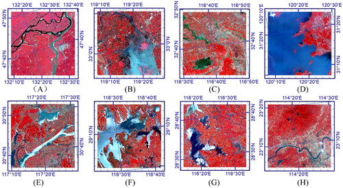
Table 1. Selected eight study areas and GF-1 satellite images.

Study areas	Landforms	Centre coordinates	Province	Regional flood year	Product serial number	Acquisition time
A: The intersection between Heilongjiang River and Songhua River	Low-altitude alluvial fan plain	132.4000E47.6895N	Heilongjiang	2013	953736	1 August 2015
B: Huaihe River downstream canal zone	Low-altitude alluvial lake plain	119.2880 E33.0237 N	Jiangsu	2007	2497326	20 July 2017
C: Huaihe River Huainan region	Low altitude alluvial plain	116.6770 E32.6732 N	Anhui	2007	2304107	13 April 2017
D: East Taihu Lake region	Low-altitude alluvial lake plain	120.3140 E31.2759 N	Jiangsu	2016	2526241	5 August 2017
E: Yangtze River Hukou below the mainstream region	Low-altitude alluvial fan plain	117.3420 E30.7299 N	Anhui	2017	2386983	28 May 2017
F: North Poyang Lake region	Low-altitude alluvial lake plain	116.5590 E29.1420 N	Jiangxi	2017	2386757	28 May 2017
G: South Poyang Lake region	Low altitude alluvial platform	116.4190 E28.5847 N	Jiangxi	2017	2386755	28 May 2017
H: Huizhou Dongjiang region	Low altitude hills& Low altitude alluvial plain	114.3510 E23.1984 N	Guangdong	2017	2217762	3 March 2017

Source: China's 1:1 million landform type data set is provided by Data Centre for Resources and Environmental Sciences, Chinese Academy of Sciences (RESDC) (http://www.resdc.cn). (Data Centre for Resources and Environmental Sciences).

3. Data

The spatial resolution, revisit cycle, scan width in satellite sensors, and flexibility in application and quality of the image data were considered. We selected GF-1 multispectral data with a spatial resolution of 8 m for the experimental data. GF-1 is the first optical satellite launched by the China High-Resolution Earth Observation System (CHEOS); it is equipped with two multispectral scanners with 2-m (panchromatic) and 8-m resolutions and a swath of over 60 km with two-camera stitching as well as four multispectral scanners with a 16-m resolution and swath of over 800 km with four-camera stitching. The multispectral data contain four bands: blue (0.45–0.52 µm), green (0.52–0.59 µm), red (0.63–0.69 µm), and near-infrared (0.77–0.89 µm). The data are characterized by a high spatial resolution, multiple spectra, a high temporal resolution, and broad coverage. Since its launch in 2013, with a revisit cycle of 4/2 days, GF-1 has provided fast, reliable, and stable optical remote sensing data for disaster mitigation in China. We selected GF-1 satellite imagery of the eight study areas from 2015 to 2017, and the data acquisition time was mainly concentrated in the flood season. Table 1 presents the product serial number and acquisition time information of the GF-1 dataset.

4. Methods

4.1. Selection and implementation of the scaling method

The scale is a fundamental and critical research issue for remote sensing and image analysis. Many scholars have used various scaling techniques depending on the type of remotely sensed images and geospatial data used. Scaling techniques affect image analysis such as object recognition and change detection (Goodchild and Quattrochi 1997; Wu and Li 2009; Weng 2014).

Different research fields define the term ‘scale’ in different ways. In ecology, the scale mainly refers to the amplitude (i.e. observation extent) and granularity (i.e. spatial resolution) (O'Neil 1998). In geography, scale primarily concerns space. However, the domains of temporal and thematic scale are also crucial (Mason 2001). Whether spatial, temporal, or thematic, the scale has several meanings in geography. The cartographic scale refers to the scale of a map. The geographic scale represents the geospatial extent of a study area. The operational scale represents the spatial extent of a particular geologic phenomenon. The measurement scale means the spatial resolution. (Quattrochi 1997; Quattrochi and Lam 2010). In this study, two scale aspects were considered: the spatial extent and spatial resolution.

Scaling techniques are divided into upscaling and downscaling. The former is the inference of low-resolution information from high-resolution variables, and the latter is the opposite (Hatfield 2001). In order to analyze the influence of different spatial extents and resolutions on the extraction accuracy of water areas, we upscaled the extent and resolution of the images to eliminate the influence of other factors and maintain consistency for the accuracy evaluation.

Remote sensing image upscaling methods are mainly statistics-based and mechanism-based. The former only considers the spatial or spectral information of the image data and does not involve the physical mechanism of the sensor imaging. Depending on the analysis unit of the image, statistics-based methods can be pixel-based (Benson and Mackenzie 1995a; Bian and Butler 1999; He et al. 2002) or object-oriented (Wu et al. 2002; Lee et al. 2011). Although a statistical model is simple and fast, it requires a large amount of sample data, and the physical meaning of the parameters is not clear (Bian and Butler 1999), which limits its practicality. In contrast, mechanism-based methods require the construction of a transformation model with multiple variables to predict the pixel values of low-resolution images from high-resolution images. Although this method is more complicated to implement than a statistics-based method, it usually has a clearer physical meaning and finer scale conversion accuracy.

One mechanism-based method for image upscaling is to simulate a point spread function (PSF) (Cracknell 1998; Stewart et al. 1998; Huang et al. 2002; Ponzoni et al. 2002). A PSF indicates the information transfer, exchange, and connection between the object space and image space in an optical system. During sensor imaging, the received signal is affected by the instantaneous field of view (IFOV) and neighbouring pixels, which are determined by the PSF effect of the sensor (Townshend 1981; Forster and Best 1994). The existence of a PSF is one of the main causes of image blurring and quality degradation (Du and Voss 2004). Therefore, a PSF can be used as a template for simulating the conversion of different scales of remote sensing images by convolution with the original image.

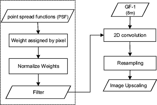
In order to maintain the intrinsic information of the original fine resolution data and match the actual effect of imaging as much as possible when the image data are converted to a coarse-resolution scale, we chose the PSF method to convert different image resolutions in the study areas. Figure 2 shows a flowchart for upscaling based on a PSF. The PSF was modelled with a Gaussian function (Stewart et al. 1998; Huang et al. 2002). A Gaussian convolution filter window was generated with the central pixel at 50% weight. The cell aggregation method was used for resampling after convolution.

Figure 2. Flow chart of scaling method based on mechanism.

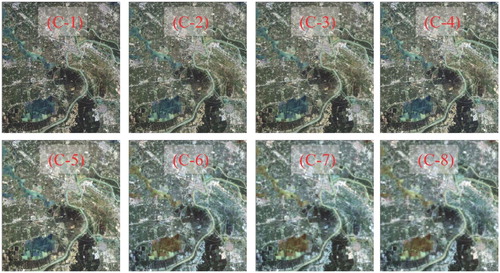
Based on the selected upscaling method, the 8 m resolution multispectral data from GF-1 were upscaled to generate a series of coarser-resolution datasets with resolutions of 24, 40, 56, 120, 152, 200, and 248 m for the study areas. The scale parameter of the different spatial resolutions was mainly selected according to two considerations: the scale parameter was an integer multiple of the original image resolution (8 m) to simplify scaling operations and ensure the same scope of the study area; and the coarse resolution obtained by the scale parameter was similar to the resolution of the existing satellite sensor data, so the findings can be applied directly to guide flood disaster monitoring. Figure 3 shows a series of datasets with different spatial resolutions for study area C (i.e. the Huaihe River Huainan floodplain) as an example.

Figure 3. Different spatial resolution series images of study area C (C-1: 8 m, C-2: 24 m, C-3: 40 m, C-4: 56 m, C-5: 120 m, C-6: 152 m, C-7: 200 m, and C-8: 248 m).

4.2. Selection of flood extraction methods

We conducted a sensitivity analysis and accuracy evaluation on different water index models for ALOS AVNIR-2 data from study area H (the Huizhou Dongjiang region): near-infrared (NIR), normalized vegetation index (NDVI), normalized differential water index (NDWI), and ratio vegetation index (RVI). The results showed that the application effects decreased in the order of NDWI, NIR, NDVI, and RVI. The overall accuracy with NDWI was close to 98% (Xiong et al. 2010). Some scholars have used the GF-1 wide field view (WFV) data for automated water classification of the Tibetan Plateau. Their results showed that using global–local segmentation with thresholds from the Otsu method (Otsu 1979) provided high quality and efficiency (Zhang et al. 2017). NDWI is the most widely used method for distinguishing between water and non-water information (Mcfeeters 1996; Xu 2006b). We used NIR, NDVI, and NDWI to extract water information for the eight study areas from the GF-1 8-m resolution data and upscaled images with different resolutions. NDWI provided better water classification than NIR and NDVI with a classification accuracy of over 98% for each study area.

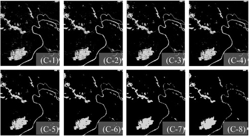
There are two considerations for water extraction. First, the thresholds of NDWI for distinguishing between water and non-water units will differ because of the different sediment concentrations in different study areas. The optimal segmentation threshold can be automatically selected for each water unit with the Otsu algorithm (Otsu 2007). Second, automatic water extraction with NDWI may include building shadows, which needs to be manually corrected by visual interpretation for the final water extraction results. As an example, Figure 4 shows a series of water body extraction results of study area C from GF-1 image data and different spatial resolutions for subsequent analysis.

Figure 4. The results of water extraction from different spatial resolution images of C study area (C-1: 8 m, C-2: 24 m, C-3: 40 m, C-4: 56 m, C-5: 120 m, C-6: 152 m, C-7: 200 m, and C-8: 248 m).

4.3. Establishment of sampling datasets with different scales

In order to study the influence of different spatial resolutions for images on the accuracy of water extraction to different extents, a series of datasets was generated through the following process. First, the water boundaries from image datasets of the eight study areas at the GF-1 8-m resolution and seven coarser spatial resolutions (24, 40, 56, 120, 152, 200, and 248 m) extracted by the upscaling and NDWI methods were used as sampling datasets. Second, the extent of the study area was changed from smaller to larger. The extent of 30 km × 30 km was divided into a series of sample grids with seven extents (0.25, 1, 4, 9, 15, 25, and 36 km² of the entire study area). Third, in each study area, the water area and proportion of the water body (PW) extracted from each coarse-resolution image in the sampling grids of different extents were counted.

4.4. Establishment of accuracy evaluation indicators

One of the objectives of this study was to examine the influence of the accuracy with the scales of the monitoring extent and spatial resolution on the extraction of regional floodwater areas by remote sensing. For this purpose, three relative accuracy indicators were adopted: the regional accuracy, average regional accuracy, and relative error.

4.4.1. Regional accuracy

The regional accuracy ($P_{\left(s,i\right)}$) was used as an indicator of the influence of the total regional accuracy on the spatial resolution. The total water area ($A_0$）extracted from the GF-1 8-m resolution multispectral data was used as the reference value (true value). The water area ($A_i$) extracted from a series of coarser-resolution ($i$) data obtained by upscaling was compared with（$A_0$）to obtain the extraction accuracy of the total water area in the region and analyze the influence of different spatial resolutions. (1) $$P_{\left(s,i\right)}=\left(1-\frac{|A_i-A_0|}{A_0}\right)\times 100\%$$(1)

4.4.2. Average regional accuracy

The average regional accuracy is the arithmetic average of the regional accuracy for all sampling grids in the sampled dataset: (2) $${\overline{P}}_{\left(s,i\right)}=\sum _{j=1}^n\raisebox{1ex}{$P_{\left(s,i\right)}$}\!\left/ \!\raisebox{-1ex}{$n$}\right.$$(2) where $s$ is a given spatial extent, $n$ is the number of sampling grids in the spatial extent dataset, $j$ is the $j$th grid, $P_{\left(s,i\right)}$ is the regional accuracy, and ${\overline{P}}_{\left(s,i\right)}$ is the average regional accuracy.

4.4.3. Relative error

The relative error (RE) measures the regional accuracy and is the ratio of the absolute error of a measurement to the measurement being taken (Golub and Van Loan 2012): (3) $$\mathrm{RE}=\frac{|A_i-A_0|}{A_0}\times 100\%$$(3)

4.5. Division of the proportion of the water body

The proportion of the water body (PW) is the percentage of the water body covering a particular spatial extent. Within the spatial extent of a study area, the PW differs for each sampling grid. This impacts the regional accuracy of the water body extraction. In order to study the variation in regional accuracy of floodwater body extraction with the spatial resolution and observation extent under different PW conditions, sampling grids of 1 km × 1 km and 2 km × 2 km were selected to calculate the PW extracted from coarser image resolutions at different spatial scales. The PW of different spatial extents was divided into five grades (<20%, 20–40%, 40–60%, 60–80%, and 80–100%) to generate a new PW dataset. The average regional accuracy of each PW dataset relative to the reference value (i.e. water body extraction results with the 8-m resolution images) was calculated for subsequent analysis.

4.6. Selection of landscape pattern indices

The landscape pattern index is an indicator for landscape patterns. It is one of the most widely used methods for quantitative analysis of the structural composition and spatial allocation of landscape patterns (Haines-Young and Chopping 1996; Fu et al. 2010). Many scholars have proposed hundreds of landscape pattern indices from different perspectives (O'Neil and Krummel 1988; McGarigal 2014); some have been used to quantify the spatial structural characteristics of water landscapes (Li et al. 2001; Wiens 2002; Tockner et al. 2010).

In order to analyze the influence of the landscape pattern on flood extraction accuracy, 18 landscape pattern indices were selected (Table 2) and calculated for 8 and 56 m resolution data with a 3 km × 3 km sampling grid of the eight study areas. Water landscape indices of 554 sampling grids were obtained in study areas A (59), B (89), C (64), D (33), E (80), F (91), G (92), and H (46). The sampling grids of non-water and all-water bodies were deleted. A correlation analysis was carried out on the relative error between the water extraction and 18 landscape pattern indices for images with 8- and 56-m resolutions in the eight study areas. Meanwhile, the 18 landscape pattern indices were calculated for image data with an 8-m resolution and 30 km × 30 km spatial extent in the eight study areas.

Table 2. Descriptions and broad definitions of selected 18 landscape pattern indices.

ID	Landscape pattern indices	Index description/definition
1	Total Water Area (TA)	TA > 0, TA equals the total area (m^2) of the corresponding water patch type
2	Total Edge (TE)	TE ≥ 0, without limit. The total length of all edges; may or may not including landscape boundary
3	Perimeter Area Ratio (PARA)	PARA >0. PARA is the ratio of total patch circumference to total patch area. It reveals the degree of patch type segmentation by the boundary and is a direct reflection of landscape fragmentation. In general, the more complex plaque shape, the higher the value of PARA
4	Number of Patches (NP)	NP ≥ 1, without limit. NP equals the number of patches of the corresponding patch type (class)
5	Largest Patch Index (LPI)	0 < LPI ≤ 100, LPI equals the area (m^2) of the largest patch of the corresponding patch type divided by total landscape area (m^2), multiplied by 100 (to convert to a percentage); in other words, LPI equals the percentage of the landscape comprised by the largest patch
6	Edge Density (ED)	ED ≥ 0, without limit. ED equals the sum of the lengths (m) of all edge segments in the landscape, divided by the total landscape area (m2), multiplied by 10,000 (to convert to hectares). Regardless of whether a landscape border is present or not, ED includes a user-specified proportion of internal background edge
7	Landscape Shape Index (LSI)	LSI ≥ 1, without limit. LSI equals the total length of edge (or perimeter) involving the corresponding class, given in number of cell surfaces, divided by the minimum length of class edge (or perimeter) possible for a maximally aggregated class, also given in number of cell surfaces, which is achieved when the class is maximally clumped into a single, compact patch
8	Patch Area Mean (AREA_MN)	AREA_MN (Mean) equals the sum, across all patches of the corresponding patch type, of the corresponding patch metric values, divided by the number of patches of the same type. MN is given in the same units as the corresponding patch metric
9	Perimeter Area Ratio Mean (PARA_MN)	PARA_MN (Mean) equals the sum, across all patches in the landscape, of the corresponding patch metric values, divided by the total number of patches. MN is given in the same units as the corresponding patch metric
10	Total Core Area (TCA)	TCA ≥ 0, without limit. TCA equals the sum of the core areas of each patch (m^2), divided by 10,000 (to convert to hectares)
11	Number of Disjunct Core Area (NDCA)	NDCA ≥ 0, without limit. NDCA equals the sum of the number of disjunct core areas contained within each patch of the corresponding patch type; that is, the number of disjunct core areas contained within the landscape
12	Clumpiness Index (CLUMPY)	−1 ≤ CLUMPY ≤1. It represents the degree of aggregation of different patch types in the landscape. It equals 0 when the patches are distributed randomly, and approaches 1 when the patch type is maximally aggregated
13	Proportion of Like Adjacency (PLADJ)	0 ≤ PLADJ ≤ 100. The percentage of cell adjacencies involving the corresponding patch type that are like adjacencies. When the patch type is the largest dispersion, and there is no similar adjacency, the PLADJ value is the smallest. When the landscape is composed of only one patch, and all adjacency is the same type, the PLADJ value is the largest
14	Patch Cohesion Index (COHESION)	0 ≤ COHESION < 100. It is the index of measuring the spatial connectivity of landscape types. The larger the COHESION, the higher the spatial connectivity of the landscape
15	Landscape Division Index (DIVISION)	0 ≤ DIVISION < 1. DIVISION equals one minus the sum of patch area (m^2) divided by total landscape area (m^2), quantity squared, summed across all patches of the corresponding patch type. Note, total landscape area (A) includes any internal background present
16	Effective Mesh Size (MESH)	the ratio of cell size to a landscape area ≤ MESH ≤ total landscape area (A). MESH equals the sum of patch area squared, summed across all patches of the corresponding patch type, divided by the total landscape area (m^2), divided by 10,000 (to convert to hectares)
17	Splitting Index (SPLIT)	1 ≤ SPLIT ≤ number of cells in the landscape squared. SPLIT equals the total landscape area (m^2) squared divided by the sum of patch area (m^2) squared, summed across all patches in the landscape
18	Normalized Landscape Shape Index (NLSI)	0 ≤ NLSI < 1.NLSI = 0 when the landscape consists of a single square or maximally compact almost square, it increases when the patch types become increasingly disaggregated and are 1 when the patch type is maximally disaggregated

Source: Gustafson (1998), Haines-Young and Chopping (1996), Kim and Pauleit (2007), McGarigal (2014), McGarigal et al. (2012), McGarigal and Marks (1995), O'Neil and Krummel (1988), O'neill et al. (1996), Turner et al. (1989).

5. Results and analysis

5.1. Influence of the spatial scale and changes in extent on the floodwater extraction accuracy

5.1.1. Effect of different spatial resolutions

The method described in Section 4.2 was used to extract the water boundary from the GF-1 8-m resolution images and images at seven other spatial resolutions. Then, the method described in Sections 4.3–4.4 was used to obtain the regional accuracy index and analyze the influence of different spatial resolutions on the extraction accuracy of the flood area. The trend of the regional accuracy index curve was similar for each study area. Table 3 presents the results of study area C as an example.

Table 3. Influence of different spatial resolution on the regional accuracy of water extraction.

Resolution (M)	8	24	40	56	120	152	200	248
Water area $A_0$ (km^2)	94.43	88.72	85.14	82.57	74.78	70.93	68.16	63.41
Regional accuracy $P_{\left(s,i\right)}$ (%)	–	93.96	90.16	87.44	79.19	75.11	72.18	67.15

For an extent of 30 × 30 km², the total area of the extracted water body gradually decreased with the spatial resolution of the data, and the regional accuracy decreased accordingly. Figure 4 compares the water extraction results of different image resolutions; the water extraction from coarse-resolution images missed some smaller water bodies and narrow rivers and ditches compared with the results using the GF-1 8-m resolution images.

5.1.2. Influence of different spatial extents

The method described in Sections 4.3–4.4 was used to obtain the average regional accuracy index, and the influence of different spatial extents and image resolutions on the extraction accuracy of the flood area was analyzed. As an example, Figure 5 shows the relationship between the average regional accuracy and different spatial extents and spatial resolutions for study area C.

Figure 5. The change of average regional accuracy with different spatial resolutions and spatial extents.

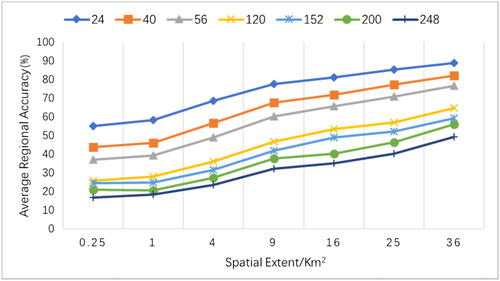
The average regional accuracy was obviously affected by the spatial resolution and spatial extent. When the spatial resolution of the image remained unchanged, the average regional accuracy increased with the spatial extent (i.e. sampling grid) of the study area. When the same spatial extent remained unchanged, the average regional accuracy decreased gradually with the spatial resolution of the image. This is consistent with the results given in Table 3.

5.1.3. Influence of different proportions of the water body

The method described in Section 4.5 was used to calculate the average regional accuracy ${\overline{P}}_{\left(s,i\right)}$ of each PW dataset relative to the reference value. The variations in the average regional accuracy of the two different spatial extents $\left(s\right)$, the seven different spatial scales ($i$), and five different PW were analyzed. The trends of the indicator curves were roughly similar in each study area. As an example, Figure 6 shows the variation in the average regional accuracy for study area C.

Figure 6. Average regional accuracy changes with different proportion of water body. (a) The average regional accuracy of 1 km². (b) the average regional accuracy of 4 km².

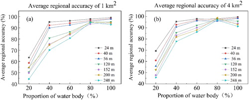
When the PW was constant, the average regional accuracy $\overline{P}$ increased with the image resolution. $\overline{P}$ generally increased with the PW at different sampling grids$\mathrm{}\left(s\right)$ and resolutions ($i$). At different resolutions, $\overline{P}$ was lowest when the PW was less than 20%. $\overline{P}$ significantly improved by about 30% when the PW rose from 20% to 40%. When the PW was at 60%–80%, $\overline{P}$ was relatively stable at spatial resolutions of 24, 40, and 56 m and reached about 95%. When PW increased to more 80%, $\overline{P}$ decreased slightly at spatial resolutions of 120, 152, 200, and 248 m to about 92%.

5.2. Influence of the landscape pattern on the floodwater extraction accuracy

5.2.1. Correlation analysis between the landscape pattern indices and relative error of the water extraction

The method described in Section 4.6 was used to calculate the landscape pattern indices for the 8- and 56-m resolution data, and the correlation with the relative error of the water extraction was analyzed. As listed in Table 4, the landscape pattern indices with a strong correlation with the relative error (i.e. an absolute value greater than 0.7) were PARA, PLADJ, COHESION, NLSI, and CLUMPY.

Table 4. Correlation between RE and landscape pattern indices with different resolution.

Landscape pattern indices	Correlation between RE and landscape index of 8 m	Correlation between RE and landscape index of 56 m
Perimeter area ratio (PARA)	0.89	0.91
Normalized landscape shape index (NLSI)	0.81	0.86
Proportion of like adjacency (PLADJ)	−0.89	−0.91
Patch cohesion index (COHESION)	−0.86	−0.91
Clumpiness (CLUMPY)	−0.74	−0.80

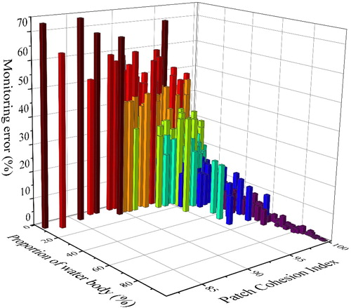
With regard to the landscape pattern, the water extraction error of the coarse-resolution (56 m) images was positively correlated with the complexity of the patch shape (i.e. PARA, NLSI) and negatively correlated with patch aggregation (i.e. PLADJ, CLUMPY) and patch connectivity (i.e. COHESION). This conclusion was verified by three-dimensional mapping of the water extraction error, PW, and landscape pattern indices such as PARA, PLADJ, and COHESION, as shown in Figures 7–9.

Figure 7. The relationship among water extraction error and proportion of water body and PARA.

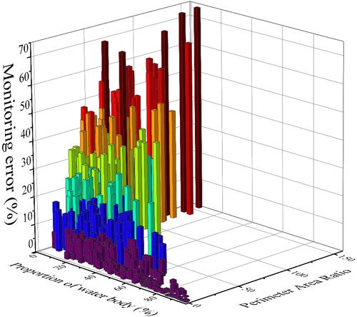
Figure 8. The relationship among water extraction error and proportion of water body and PLADJ.

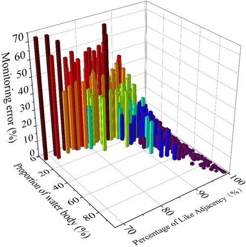
Figure 9. The relationship among water extraction error and proportion of water body and COHESION.

5.2.2. Improving the floodwater extraction accuracy with the landscape pattern index

Based on the correlation analysis between the landscape pattern indices and relative error of the floodwater surface extraction, PARA was selected as the standard because it had the strongest correlation with the relative error. K-means cluster analysis was used to classify the water patches extracted from the 8-m and 56-m resolution images of the 554 sampling grids into three categories according to the complexity of the patch shape: low, medium and high. The total water area was also calculated at the 8- and 16-m resolutions. Table 5 clearly indicates that the relative error of the water extraction increased significantly as the complexity of the water patch shape increased in the study areas.

Table 5. Results of water body area with different patch shape complexity.

Patch shape complexity	Number of grids	$A_0$	$A_{56}$	Relative error (%)
Low	298	1105.82	1073.6	−2.91
Medium	197	227.36	183.95	−19.09
High	59	35.57	20.58	−42.14

The landscape pattern has a significant impact on the floodwater extraction accuracy. A multivariate regression equation was established between the floodwater extraction for different levels of patch shape complexity in the coarse-resolution images and the landscape pattern indices to simulate the water extraction from finer resolution images. The purpose was to improve the accuracy of water extraction from coarse-resolution image data.

Because the two measurement variables (i.e. the water area extraction results from the 8- and 56-m resolution images) did not fit a normal distribution, the square-root transformation (Bartlett 1936) was applied so that they would conform to a normal distribution test. The transformed 8-m resolution results for the water extraction were taken as the dependent variable, and the transformed 56-m resolution results for the water extraction and the corresponding 18 landscape pattern indices were taken as independent variables. The stepwise method (forward) (Hocking 1976; Hinton et al. 2004) was used to screen out significant factors affecting the dependent variable, and a corresponding multiple regression model was established. Table 6 presents the regression model parameters of three different patch complexities. In contrast with the simple linear regression model that used only the water area at a 56-m resolution as the variable, landscape pattern indices were used as the variables for the multiple regression analysis. For regions with highly complex patch shapes, the correlation coefficient (R) of the regression equation increased from 0.85 to 0.94, and the correlation coefficient (R) for regions with patch shapes of medium and low complexity stayed at 0.99. The results showed that the water extraction accuracy for highly complex patch shapes could be significantly improved by using the landscape index as an independent variable for coarse-resolution data.

Table 6. A multivariate regression equation parameters.

	Low patch complexity				Medium patch complexity				High patch complexity
	B	Std. err	t	Sig.	B	Std. err	t	Sig.	B	Std. err	t	Sig.
Constant	−452.27	71.66	−6.31	0.00	68.02	23.42	2.90	0.00	213.72	21.06	10.15	0.00
water area with 56M	0.98	0.003	302.48	0.00	0.88	0.03	31.93	0.000	0.72	0.05	15.34	0.00
Number of plaques	1.82	0.25	7.29	0.00	3.24	0.34	9.62	0.000	6.77	0.78	8.71	0.00
PARA	5.87	1.18	4.98	0.00	–	–	–	–	–	–	–	–
PLADJ	2.12	1.02	2.08	0.04	4.11	2.03	2.03	0.04	–	–	–	–
COHESION	3.10	0.90	3.45	0.00	–	–	–	–	–	–	–	–
Boundary perimeter	0.00	0.00	−2.97	0.00	–	–	–	–	–	–	–	–
PARA_mean	–	–	–	–	0.18	0.03	5.68	0.00	–	–	–	–
Average patch area	–	–	–	–	2.29	0.66	3.48	0.00	–	–	–	–
CLUMPY	–	–	–	–	−410.54	172.40	−2.38	0.02	–	–	–	–

5.3. Data selection for regional flood monitoring by remote sensing of different landscape patterns

The analysis presented in the above sections showed that the spatial resolution of the remote sensing data, PW, and the landscape pattern had a significant impact on the accuracy of the water body extraction at a given spatial extent. Table 7 presents the PW, five significant landscape pattern indices (i.e. PARA, NLSI, PLADJ, COHESION, and CLUMPY), and the regional accuracy of the water body extraction at seven spatial resolutions of a spatial extent of 30 km × 30 km in each of the eight study areas. A comparative analysis was performed to find the optimal spatial resolution of the water body extraction for remote sensing of regional flood disasters in the study areas.

Table 7. Regional accuracy of water extraction with the proportion of water body, the landscape pattern indices, and different spatial resolution images.

Study area（30 km × 30 km）	Proportion of water	PARA	NLSI	COHESION	PLADJ	CLUMPY	Regional accuracy of different spatial resolution（%）
	(%)			(%)	(%)		24 m	40 m	56 m	120 m	152 m	200 m	248 m
A: Intersection between Heilongjiang River and Songhua River	10.02	17.32	0.03	99.86	96.53	0.96	96.73	93.56	90.13	77.06	72.37	65.89	60.27
B: Huaihe River downstream canal zone	31.09	21.13	0.04	99.69	95.76	0.94	96.93	94.55	92.46	85.95	83.39	81.13	76.50
C: Huaihe River Huainan region	10.49	28.31	0.06	99.33	94.31	0.94	93.96	90.16	87.44	79.19	75.11	72.18	67.15
D: East Taihu Lake region	70.33	2.06	0.01	99.94	99.57	0.99	99.53	99.29	99.20	97.82	97.44	96.55	95.67
E: Yangtze River Hukou below main stream region	17.23	41.04	0.07	99.13	92.93	0.92	94.78	91.39	88.46	80.43	77.64	75.11	72.54
F: North Poyang Lake region	43.80	9.12	0.02	99.92	98.16	0.97	99.30	98.64	98.09	95.61	94.58	93.17	92.16
G: South Poyang Lake region	24.30	15.48	0.03	99.73	96.90	0.96	97.70	95.62	93.80	87.85	84.97	81.71	77.55
H: Huizhou Dongjiang River	5.93	35.77	0.07	98.06	92.83	0.92	89.95	82.87	77.27	64.09	60.17	55.12	52.51

The three landscape pattern indices (i.e. COHESION, PLADJ, and CLUMPY) did not significantly differ for the eight study areas, whereas the PW, PARA, and NLSI significantly differed. Study areas A, B, and D had a low PW (<11%), study areas E, G, and B had a medium PW (17–32%), and study areas D and F had a high PW (>43%). Study areas D and F had the lowest shape complexity, study areas G, A, and B had low shape complexity, and study areas C, H, and E had higher shape complexity.

The PW and shape complexity of the patches differed in the eight study areas. Therefore, the spatial resolution differed under certain regional accuracy constraints. For example, if the regional water extraction accuracy must be no less than 80% for flood emergency monitoring, an extraction accuracy of >90% can be achieved for study areas D and F (i.e. high PW and low shape complexity) at a coarse spatial resolution of 248 m. In contrast, study areas G and B require a spatial resolution of 200 m, study area E requires a spatial resolution of 120 m, study areas A and C require a spatial resolution of 56 m, and study area H requires a spatial resolution of 40 m.

6. Conclusion

In this study, the water extraction accuracy from multiscale remote sensing monitoring of flood disasters with different landscape patterns was simulated and analyzed. Based on GF-1 8-m resolution multispectral satellite data from eight study areas in China, a series of coarse-resolution image datasets was generated with the mechanism-based upscaling method. The water boundary from images of different resolutions was extracted with the NDWI method, and results for different extents and spatial resolutions were generated. Based on the regional water extraction accuracy and water landscape pattern indices, the influence of different spatial resolutions, spatial extents, and PW on the water body extraction accuracy was analyzed. The optimal spatial resolution was obtained for the eight study areas to obtain a fixed water extraction accuracy. The following conclusions were obtained:

1. The regional accuracy of the floodwater extraction decreased with the spatial resolution when the spatial extent was unchanged. The error of the water extraction area increased, and some small areas of water were neglected. In contrast, the average regional accuracy of the floodwater body gradually increased with the spatial extent when the spatial resolution was fixed.

2. The PW had a significant impact on the accuracy of the regional water extraction. The average regional accuracy generally increased with the PW for different spatial extents and resolutions.

3. The landscape pattern of the water body had a significant impact on regional floodwater extraction accuracy. There was a strong positive correlation between the water extraction error and complexity of the patch shape (i.e. PARA, NLSI) and a strong negative correlation with patch aggregation (i.e. PLADJ, CLUMPY), patch connectivity (i.e. COHESION), and the PW.

4. To monitor the floodwater bodies in the eight study areas, image data with different spatial resolutions should be selected according to differences in the water landscape patterns (e.g. PW and patch shape complexity) for a given water body extraction accuracy. For example, if the regional water body extraction accuracy should be no less than 80%, the spatial image resolutions should be at least 56 m for study areas A and C, 200 m for study areas B and G, 248 m for study areas D and F, 120 m for study area E, and 40 m for study area H.

For the remote sensing monitoring of regional flood disasters, the spatial scale, extent, and landscape pattern directly affect the accuracy of the flood area estimation. The main contribution of this study was to provide experimental conclusions on the relationship between water extraction accuracy and selected spatial resolution of remote sensing data for multiscale regional flood monitoring in China. Simulation data at coarse resolutions obtained by the scale expansion method were compared and analyzed. In the future, we will compare our findings with the regional water body extraction accuracy of existing commercial data with multiple spatial resolutions in order to verify the accuracy and reliability of our conclusions.

Acknowledgements

We thank the anonymous reviewers for their helpful comments on an earlier draft of this paper. Their thoughtful suggestions helped improve our work.

Disclosure statement

No potential conflict of interest was reported by the authors.

Additional information

Funding

This work was supported by the National Key Research and Development Program of China [2016YFC0803004, 2017YFB0504101], National Natural Science Foundation [41301501], and Youth Innovation Promotion Association of CAS [2015129].

References

- Amiri BJ, Gao JF, Fohrer N, Mueller F, Adamowski J. 2018. Regionalizing flood magnitudes using landscape structural patterns of catchments. Water Resour Manage. 32(7):2385–2403.
- Aplin P. 2004. Spatial variation in land cover and choice of spatial resolution for remote sensing. Int J Remote Sens. 25:3687–3702.
- Bartlett M. 1936. The square root transformation in analysis of variance. Suppl J Roy Stat Soci. 3(1):68–78
- Benson BJ, Mackenzie MD. 1995. Effects of sensor spatial resolution on landscape structure parameters. Landscape Ecol. 10(2):113–120.
- Bian L, Butler R. 1999. Comparing effects of aggregation methods on statistical and spatial properties of simulated spatial data. Photogrammet Eng Remote Sens. 65:73–84.
- Biggin DS. 2010. A comparison of ERS-1 satellite radar and aerial photography for river flood mapping. Water Environ J. 10:59–64.
- Bilskie MV, Hagen SC, Medeiros SC, Passeri DL. 2014. Dynamics of sea level rise and coastal flooding on a changing landscape. Geophys Res Lett. 41(3):927–934.
- Chen ZG. 2017. Flooded area classification by high resolution SAR images. Wuhan University.
- Cracknell AP. 1998. Review article Synergy in remote sensing – what's in a pixel? Int J Remote Sens. 19(11):2025–2047.
- Data Center for Resources and Environmental Sciences, C.R. The China's 1:1 million landform type data set. http://www.resdc.cn.
- de Andrade MMN, Szlafsztein CF. 2018. Vulnerability assessment including tangible and intangible components in the index composition: an Amazon case study of flooding and flash flooding. Sci Total Environ. 630:903–912.
- Du H, Voss KJ. 2004. Effects of point-spread function on calibration and radiometric accuracy of CCD camera. Appl Opt . 43(3):665–670.[InsertedFromOnline.
- Feyisa GL, Meilby H, Fensholt R, Proud SR. 2014. Automated water extraction index: a new technique for surface water mapping using Landsat imagery. Remote Sens Environ. 140:23–35.
- Forster BC, Best P. 1994. Estimation of SPOT P-mode point spread function and derivation of a deconvolution filter. Isprs J Photogrammet Remote Sens. 49:32–42.
- Fu BJ, Xu YD, Lv YH. 2010. Scale characteristics and coupled research of landscape pattern and soil and water loss. Adv Earth Sci. 25:673–681.
- Gianinetto M, Villa P, Lechi G. 2005. Postflood damage evaluation using Landsat TM and ETM + data integrated with DEM. IEEE Trans Geosci Remote Sens. 44:236–243.
- Golub GH, Van Loan CF. 2012. Matrix computations. JHU Press.
- Goodchild MF, Quattrochi DA. 1997. Scale, multiscaling, remote sensing, and GIS.
- Gustafson EJ. 1998. Quantifying landscape spatial pattern: what is the state of the art? Ecosystems. 1(2):143–156.
- Haibo Y, Zongmin W, Hongling Z, Yu G. 2011. Water body extraction methods study based on RS and GIS. Procedia Environ Sci. 10:2619–2624.
- Haines-Young R, Chopping M. 1996. Quantifying landscape structure: a review of landscape indices and their application to forested landscapes. Prog Phys Geogr. 20(4):418–445.
- Hatfield J. 2001. Upscaling and downscaling methods for environmental research. J Environ Qual. 30(3):1100.
- He HS, Ventura SJ, Mladenoff DJ. 2002. Effects of spatial aggregation approaches on classified satellite imagery. Int J Geogr Inform Sci. 16(1):93–109.
- Hinton PR, McMurray I, Brownlow C. 2004. SPSS explained. Routledge.
- Hlavka C, Dungan J. 2002. Areal estimates of fragmented land cover: effects of pixel size and model-based corrections. Int J Remote Sens. 23(4):711–724.
- Hocking RR. 1976. A biometrics invited paper. The analysis and selection of variables in linear regression. Biometrics. 32(1):1–49.
- Horritt MS, Mason DC, Luckman AJ. 2001. Flood boundary delineation from synthetic aperture radar imagery using a statistical active contour model. Int J Remote Sens. 22(13):2489–2507.
- Huang CQ, Townshend JRG, Liang SL, Kalluri SNV, DeFries RS. 2002. Impact of sensor's point spread function on land cover characterization: assessment and deconvolution. Remote Sens Environ. 80(2):203–212.
- Ji L, Zhang L, Wylie B. 2009. Analysis of dynamic thresholds for the normalized difference water index. Photogramm Eng Remote Sens. 75:1307–1317.
- Kim K-H, Pauleit S. 2007. Landscape character, biodiversity and land use planning: the case of Kwangju City Region, South Korea. Land Use Policy. 24(1):264–274.
- Lee S-H, Lim S-Y, Kim N, Park N-C, Yang H, Park K-S, Park Y-P. 2011. Increasing the storage density of a page-based holographic data storage system by image upscaling using the PSF of the Nyquist aperture. Opt Express. 19(13):12053. 12065
- Leng Y, Li N. 2017. Improved change detection method for flood monitoring. J Radars. 6:204–212.
- Li J, Zhou Q, Chen X, Ling Tian QL, Li TY. 2018. Spatial sale study on quantitative remote sensing of highly dynamic coastal/inland waters. Geomat Inform Sci Wuhan Univ. 43:937–942.
- Li JG, Huang SF, Li JR. 2010. Research on extraction of water body from ENVISAT ASAR images: a modified Otsu threshold method. J Nat Disasters. 19:139–145.
- Li X, Lu L, Cheng G, Xiao H. 2001. Quantifying landscape structure of the Heihe River Basin, north-west China using FRAGSTATS. J Arid Environ. 48(4):521–535.
- Lv YH, Chen LD, Fu BJ. 2007. Analysis of the integrating approach on landscape pattern and ecological processes. Prog Geogr. 26:1–10.
- Marceau DJ, Hay GJ. 1999. Remote sensing contributions to the scale issue. Can J Remote Sens. 25(4):357–366.
- Mason A. 2001. Unresolved issues. J Econ Perspect. 2:41–58.
- Mcfeeters SK. 1996. The use of the Normalized Difference Water Index (NDWI) in the delineation of open water features. Int J Remote Sens. 17(7):1425–1432.
- McGarigal K. 2014. Landscape pattern metrics. Wiley StatsRef: Statistics Reference Online.
- McGarigal K, Cushman SA, Ene E. 2012. FRAGSTATS v4: spatial pattern analysis program for categorical and continuous maps. Computer software program produced by the authors at the University of Massachusetts, Amherst. http://www.umass.edu/landeco/research/fragstats/fragstats.html.
- McGarigal K, Marks BJ. 1995. FRAGSTATS: spatial pattern analysis program for quantifying landscape structure. Gen. Tech. Rep. PNW-GTR-351. Portland, OR: US Department of Agriculture, Forest Service, Pacific Northwest Research Station. 122 p, 351
- Moody A, Woodcock CE. 1994. Scale-dependent errors in the estimation of land-cover proportions: implications for global land-cover datasets. Photogramm Eng Remote Sens. 60:585–596.
- Moody A, Woodcock CE. 1995. The influence of scale and the spatial characteristics of landscapes on land-cover mapping using remote sensing. Landscape Ecol. 10(6):363–379.
- NCDR. 2016. The action of China's Disaster Reduction during “12th Five-Year Plan” period. NCDR
- O'Neil R. 1998. Homage to St. Michael: or, why are there so many books on scale? Ecol Scale.
- O'Neil R, Krummel J. 1988. Indices of landscape pattern. Landscape Ecol. 1.
- O'Neill R, Hunsaker C, Timmins SP, Jackson B, Jones K, Riitters KH, Wickham JD. 1996. Scale problems in reporting landscape pattern at the regional scale. Landscape Ecol. 11:169–180.
- Orman US. 2001. Determination of flood inundated areas using RS techniques in the western Black Sea Region of Turkey. Turk J Eng Environ Sci. 25:379–389.
- Otsu N. 1979. A threshold selection method from gray-level histograms. IEEE Trans Syst Man Cybern. 9:62–66.
- Otsu N. 2007. A threshold selection method from gray-level histograms. IEEE Trans Syst Man Cybern. 9:62–66.
- Ponzoni J, Galvão F, Epiphanio LS, José CN. 2002. Spatial resolution influence on the identification of land cover classes in the Amazon environment. An Acad Bras Cienc. 74:196–198.
- Quattrochi CA. 1997. Scale in remote sensing and GIS. Lewis Publishers.
- Quattrochi DA, Lam NSN. 2010. On the issues of scale, resolution, and fractal analysis in the mapping sciences. Prof Geogr. 44:88–98.
- Rahman MS, Di LP. 2017. The state of the art of spaceborne remote sensing in flood management. Nat Hazards. 85(2):1223–1248.
- Rango A, Anderson AT. 1974. Flood hazard studies in the Mississippi river basin using remote sensing. J Am Water Resources Assoc. 10(5):1060–1081.
- Raptis V, Vaughan R, Wright G. 2003. The effect of scaling on land cover classification from satellite data. Comput Geosci. 29:705–714.
- Read JM, Lam SN. 2002. Spatial methods for characterising land cover and detecting land-cover changes for the tropics. Int J Remote Sens. 23(12):2457–2474.
- Smith JH, Stehman SV, Wickham JD, Yang L. 2003. Effects of landscape characteristics on land-cover class accuracy. Remote Sens Environ. 84(3):342–349.
- Stewart JB, Engman ET, Feddes RA, Kerr YH. 1998. Scaling up in hydrology using remote sensing: summary of a Workshop. Int J Remote Sens. 19(1):181–194.
- Takeuchi S, Konishi T, Suga Y, Kishi S. 1999. Comparative study for flood detection using JERS-1 SAR and Landsat TM data. Geoscience and Remote Sensing Symposium, 1999. IGARSS '99 Proceedings. IEEE 1999 International. Vol. 872. p. 873–875.
- Tockner K, Lorang MS, Stanford JA. 2010. River flood plains are model ecosystems to test general hydrogeomorphic and ecological concepts. River Res App. 26(1):76–86.
- Townshend JRG. 1981. Spatial resolution of satellite images. Prog Phys Geogr. 5.
- Townshend JRG, Justice CO. 1988. Selecting the spatial resolution of satellite sensors required for global monitoring of land transformations. Int J Remote Sens. 9(2):187–236.
- Turner MG, O'Neill RV, Gardner RH, Milne BT. 1989. Effects of changing spatial scale on the analysis of landscape pattern. Landscape Ecol. 3(3–4):153–162.
- Wang FT, Wang SX, Zhou Y. 2011. Application and prospect of multi-spectral remote sensing in major natural disaster assessment. Spectrosc Spect Anal. 31:577–582.
- Wei CJ, Wang SX. 1998. The role of remote sensing technology in monitoring and evaluation of flood disaster in China. Bull Chinese Acad Sci. 13:443–447.
- Weng Q. 2014. Scale issues in remote sensing. John Wiley & Sons.
- Wiens JA. 2002. Riverine landscapes: taking landscape ecology into the water. Freshwater Biol. 47(4):501–515.
- Woodcock CE, Strahler AH. 1987. The factor of scale in remote sensing. Remote Sens Environ. 21(3):311–332.
- Wu H, Li Z-L. 2009. Scale issues in remote sensing: a review on analysis, processing and modeling. Sensors. 9(3):1768–1793.
- Wu J, Shen W, Sun W, Tueller PT. 2002. Empirical patterns of the effects of changing scale on landscape metrics. Landscape Ecol. 17(8):761–782.
- Xiong JG, Wang SX, Zhou Y. 2010. A sensitivity analysis and accuracy assessment of different water extraction index models based on ALOS AVNIR-2 data. Remote Sens Land Resour. 22:46–50.
- Xu H. 2006. Modification of normalised difference water index (NDWI) to enhance open water features in remotely sensed imagery. Int J Remote Sens. 27(14):3025–3033.
- Yamagata Y, Akiyama T. 1988. Flood damage analysis using multitemporal Landsat Thematic Mapper data. Int J Remote Sens. 9(3):503–514.
- Zhang G, Zheng G, Gao Y, Xiang Y, Lei Y, Li J. 2017. Automated water classification in the Tibetan plateau using Chinese GF-1 WFV data. Photogramm Eng Remote Sens. 83(7):509–519.
- Zhang H, Xu XY, Zhang L, Wang HR. 2011. Comprehensive assessment of loss of flood and water logging disasters from 2000 to 2010 and analysis of their causes. J Econom Water Resour. 29:5–9.
- Zhang M, Li Z, Tian B, Zhou J, Tang P. 2016. The backscattering characteristics of wetland vegetation and water-level changes detection using multi-mode SAR: a case study. Int J Appl Earth Obs Geoinform. 45:1–13.
- Zhang SJ. 2005. Research on remote sensing monitoring and disaster evaluation of flood disaster. Nanjing University of Information Science and Technology.