
 ?Mathematical formulae have been encoded as MathML and are displayed in this HTML version using MathJax in order to improve their display. Uncheck the box to turn MathJax off. This feature requires Javascript. Click on a formula to zoom.
Abstract
This article puts forward an algorithm for estimating the detection efficiency (DE) of a lightning location system (LLS). The algorithm can be applied to lightning flash/stroke density correction and LLS performance evaluation. Fundamentally, the generalized extreme value (GEV) distribution was found to best fit the probability distribution of the signal strengths of the lightning observed by the ADvanced TOA and Direction system (ADTD) detectors in Beijing, China. With respect to this probability distribution, we estimated the single-station acceptance damped by the uneven underlying land surface conductivity, which is determined by overlapping the soil-type polygons with the propagating paths of electromagnetic lightning signals. Accounting for the multi-detector location modes supported by single-station acceptance, the iterative algorithm was applied for deducing the network DE. In this case study, the DE estimates were lower in the mountainous areas than in the plains. This can be due to the low underlying conductivity of the mountainous areas, which creates a high attenuation effect on the lightning electromagnetic signals, and the greater distances from the lightning detectors. The CG lightning flash/stroke density corrected for the DEs revealed that the CG lightning flash/stroke densities in the mountains are lower than that in the highly urbanized plains.
1. Introduction
Lightning location systems (LLSs) capture natural lightning electromagnetic signals and consequently locate lightning sources. LLS observations can be used to derive and retrieve lightning parameters that indicate lighting characteristics, e.g. the cloud-to-ground (CG) lightning flash density, the positive/negative CG flash/stroke density, the percent of positive/negative flashes, the first stroke negative and positive peak currents, and the multiplicity for negative and positive flashes (Orville et al. Citation2002; Citation2011; Rudlosky and Fuelberg Citation2010; Taszarek et al. Citation2015). These types of data have been widely used in weather forecasting, severe weather warning systems and climatological analysis, e.g. assimilation in weather forecasting models (e.g. Fierro et al. Citation2011; Fierro and Reisner Citation2011), synoptic analysis of thunderstorms (e.g. Changnon Citation1993; Cummins and Murphy Citation2009), presentations of lightning characteristics (e.g. Schulz et al. Citation2005; Drüe et al. Citation2007; Mäkelä et al. Citation2010), lightning climatology and climate pattern recognition (e.g. Antonescu and Burcea Citation2010; Williams Citation2005; Taszarek et al. Citation2015; Etherington and Perry Citation2017), and lightning risk assessment (Hu et al. Citation2014). However, a serious problem emerges when a LLS provides an inhomogeneous detection efficiency (DE) within the detectable distance or even a very low DE at the edges of the detectable distance (Naccarato and Pinto Citation2009), which greatly restricts the applicability of the LLS data (Hu et al. Citation2014; Yao et al. Citation2012).
DE is determined by the performance and sensitivity of the sensors, the sensor network geometry, the underlying ground conductivity (Schütte et al. Citation1988; Naccarato and Pinto Citation2009; Mäkelä et al. Citation2010), etc. The unevenly distributed DEs contribute to LLS data uncertainty and ruin data validity (Williams Citation2005; Yao et al. Citation2012; Hu et al. Citation2014). Thus, it is desirable to further develop algorithms to estimate the DE, which can be applied for correcting the lightning flash/stroke density derived from the LLS data.
Moreover, such an algorithm is useful in LLS performance evaluation and network deployment validation and would help to determine optimal detector deployment (Cummins et al. Citation1998; Idone et al. Citation1998; Schulz et al. Citation2005). This methodology was originally intended to test network deployment optimization and network performance and eventually became applicable to improve LLS data quality. Schütte et al. (Citation1987, Citation1988) suggested that the lightning impulse signal strength (LISS) weakens linearly with propagation distance and confirmed the Weibull probability distribution of LISSs received by a single station within a detectable distance. Naccarato and Pinto (Citation2009) estimated the DE of the Brazilian lightning detection network (BrasilDAT) based on the individual sensor DE probability functions, which were derived from a large amount of CG stroke data provided by the network.
Methodologically, Naccarato and Pinto (Citation2009) estimated the BrasilDAT DE based on the sensor individual DE probability functions, which are derived from a large amount of CG stroke data provided by the network considering different distances from the sensor and specific peak current ranges, and minimized the unrealistic enhancement of the DE closer to the network boundaries. Their method can be briefly described as: (1) One smaller region (450 × 450 km) region was chosen as the center quad (QUAD) area, which was used to assess the reference cumulative peak current distribution (PCD); (2) The coverage area of the LDN was divided into blocks and the number of CG lightning flashes was computed for each block. The PCD for each cell was computed individually and adjusted to the reference PCD. The ratio between the adjusted and the reference PCD at the 0 kA axis corresponded to the RFDE of the network in that cell. Schütte et al. (Citation1988) assumed that the distribution of lightning signal strengths is that of Weibull distribution, and the acceptance of each sensor in the network could be the cumulative probability of detected signal strength range. The damping model for signal propagation, considering the acceptance/distance relationship for different ground conductivities was also taken into account (Schütte et al. Citation1987). Then, the acceptance of lightning detectors can be calculated knowing the lightning signal-strength distribution, the receiver thresholds, and the damping conditions for the propagation of lightning pulses.
These applicable approaches obviously possess reference values in the aftermath of DE estimation. Note that the precedent work can be cited as a referential source; however, it is inappropriate to simply copy the methods of earlier researchers if considering different data resources and circumstances. For example, the Weibull distribution of LISSs identified by Schütte et al. (Citation1987, Citation1988) only reflected the lightning characteristics observed by the European LLS network at that time. However, our study revealed that the probability distribution of the LISSs detected by the ADTD sensors deployed around Beijing, China, would fit the generalized extreme value (GEV) distribution, rather than the Weibull distribution. This finding demonstrates the necessity of modifying the precedent methodology to estimate single-station acceptance.
Moreover, the DE and location accuracy of a LLS can be influenced by the lightning location mode, which is defined as the number of detectors synchronously receiving the lightning electromagnetic signal in one lightning location. The algorithm should consider the multi-detector location mode related to the number of detectors in the lightning location. Usually, at least two magnetic direction finder (MDF) detectors and three time-of-arrival (TOA) detectors are needed in each lightning location (Schütte et al. Citation1988). As observed by a LLS network with newly upgraded IMPACT detectors (combined MDF and TOA technology), a lightning source can be located with signals synchronously detected by two or more such detectors (Bourscheidt et al. Citation2012). With multi-detector location modes, here, an iterative algorithm is introduced to derive the DE from single-station acceptance.
Underlying surface conductivity plays an important role in damping lightning signals and eventually influences the DE (Honma et al. Citation1998; Rudlosky and Fuelberg Citation2010). Schütte et al. (Citation1987) suggested that land surface damping influences both the DE and location accuracy and that the TOA network appears more sensitive to land surface damping. At this point, the algorithm should consider the damping effect on signal strength, which is induced by land surface conductivity.
The algorithm was constructed by following the above mentioned fundamentals. In this methodology, the LISSs were calculated using a linear signal propagation model suggested by Cummins et al. (Citation1998). The damping coefficients in a grid system were estimated by addressing the land surface conductivity of specific land use and land cover (LULC) types. After correcting the signal strength magnitudes of the damping factor, we identified the GEV probability distribution of the LISSs. Based on this probability density function (PDF), we estimated the single-station acceptance of lightning source signals and ultimately calculated the grid DEs using an iterative algorithm. We corrected the CG lightning stroke density for the DEs and found an improvement in the estimates of the CG lightning stroke density in comparison with the uncorrected density.
Admittedly, the uncertainty cannot be reduced completely through DE estimation because the DE estimation fundamentals involve simulating signal attenuation propagated over certain distances and dampening due to land surface conductivity. The improvement in the LLS data quality (e.g., DE and location accuracy) basically depends on the implementation of optimal detector deployments and detector upgrading, and DE estimates are critical in promoting the applicability of the LLS data.
2. Data description
The LLS data collected from 2007–2016 by the ADTD (Advanced TOA and Direction system, where TOA denotes time-of-arrival) network deployed by the China Meteorology Administration (CMA) were used to (1) identify the probability distribution of the LISSs and (2) derive the CG flash/stroke density, which is corrected for the DE. These data include the time, location, amperage and polarity of the CG lightning strokes.
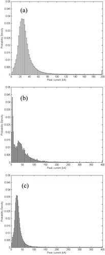
The ADTD consists of more than 301 sensors (as of March 2011) in China (Yao et al. Citation2012). In Beijing, 9-14 ADTD-1 sensors (improved IMPACT (combined MDF and TOA) sensors) can detect 1–450 kHz (very low-frequency (VLF)/low-frequency (LF) band) lightning sources (). The ADTD-1 sensors use the combined MDF and time-of-arrival (TOA) method for position retrieval (Ma Citation2015). In this method, if a lightning source is only detected by two ADTD-1 sensors, the algorithm uses one TOA hyperbolic curve and two MDF vectors to retrieve the position. If a lightning source is detected by three sensors in a non-duplicate region, the TOA algorithm is used to retrieve the position directly. In contrast, if the TOA is the first to find a duplicate location, then the MDF method is used to identify the true location. If a lightning event is detected by four or more sensors, a TOA least squares method is used to find a more precise location. Thus, a lightning location detected by four or more sensors is more precise than that detected by fewer sensors. In the ADTD data, the percentage of lightning sources reported by four or more sensors relative to the total number of detected sources is 63.3%. Meanwhile, the ADTD-observed + CG and –CG lightning peak currents are in the ranges of 0.08 kA to 995.9 kA and 0.258 kA to 992.6 kA, respectively (). Ma (Citation2015) concluded that the peak current estimates between 10 kA and 100 kA could be relatively consistent with ground truth currents, while the estimates (<10 kA or >100 kA) are 23% lower than ground truth peak current measurements.
Figure 1. Histogram of the peak current probability density of (a) the –CG lightning, (b) +CG lightning and + IC lightning identified from their peak currents less than 15 kA and (c) the total CG lightning.
The ADTD sensor manufacturers claim that the DE of the ADTD sensors could be 90% at distances between 300 and 600 km, with a median location accuracy error of 1 km. However, only the flash DE can be 90%, and the stroke detection efficiency (SDE) is lower. The first stroke peak current in a multiple-stroke CG flash can be greater than twice its subsequent stroke peak current (Rakov and Uman Citation1990). Thus, the sensors can capture the first larger peak stroke but miss the weaker subsequent stroke (Rudlosky and Fuelberg Citation2010). Moreover, some weak CG strokes (including single-stroke CG flashes) cannot be detected due to the signal attenuation induced by long-distance propagation and damping effects in lower conductivity mountainous regions (Schütte et al. Citation1988).
We estimated the SDEs of the ADTD in a grid system (1 km × 1 km, see ) and corrected the lightning stroke density using the SDE. The SDE estimates approximate those of the U.S. NLDN (National Lightning Detection Network) in 1998, which was reported to be 62% (Idone et al. Citation1998). Hence, the DE level of the ADTD is equivalent to that of the NLDN, at least in 1998, suggesting that a considerable potential for improvement remains in terms of network upgrades and that DE estimation is necessary for promoting the applicability of the ADTD data.
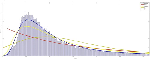
Figure 2. Fitted probability density function curves for (a) the Weibull (red line), (b) the log normal (light yellow line), (c) the extreme value (deep yellow line) and (d) the GEV (blue line) distributions of the LISSs with the histogram of the sample data.
3. Method
The probability distribution of the LISSs is critical in estimating single-station acceptance. Being prior probability distribution, it can be deduced using samples of lightning location data. The likely probability distribution of these data would be that of either the Weibull, generalized extreme value (GEV), lognormal (LN), extreme value (EV) or gamma distribution (Schütte et al. Citation1988; Evans et al. Citation1993). Hereinafter, the GEV distribution is primarily introduced (Refer to the literature of Evans et al. (Citation1993) to see the fundamentals of the other distributions). As we found in the latter, the GEV would provide the fittest probability distribution of the LISSs in the Beijing region.
3.1. GEV distribution
The GEV distribution has a cumulative distribution function (CDF)
(1)
(1)
for
where
is the location parameter,
is the scale parameter and
is the shape parameter. Thus, for
the CDF is only valid when
for
the CDF is valid and has a short-tailed Gumbel distribution when
For
the CDF is formally undefined and can be replaced by the result obtained by taking the limit as
Then,
(2)
(2)
with no restriction on x.
The density distribution function is consequently
(3)
(3)
When the density is positive over the entire real line and equal to the Weibull distribution:
(4)
(4)
3.2. Fundamentals of the GEV distribution applied for estimating single-station acceptance
Consider a normalized (for example, to a distance of 100 km), undamped reference signal-strength distribution with the frequency function f(s0) and an expression for the signal strength dependence on the distance s0 =D−1(s), where s0 is the signal strength normalized to a standard distance r0. The simplest case for an undamped radiation field is the inverse power law s= s0r0/r, expressing the signal-strength attenuation with distance r, where s is the signal-strength. The acceptance, A(r), defined as the percentage of detected cloud-to-ground lightning flashes (Schütte et al. Citation1987), can be calculated as a function of lightning signal strength distribution f(s0), the distance r and the lower and upper signal-strength thresholds smin and smax, respectively:
(5)
(5)
For undamped propagation, we can obtain
(6)
(6)
In the case of the GEV distribution, combined with EquationEqs. (1)(1)
(1) and Equation(6)
(6)
(6) , the acceptance is given by
(7)
(7)
where c is the signal bias and can be replaced by the minimum value of the signal samples.
The effective radius, describing the properties of a lightning counter or direction finder can be defined as
(8)
(8)
This definition means that an ideal lightning counter accepts all lightning signal s with and none with
When the signal strength is GEV distributed and the counter has as a sufficient dynamic range (smin ≪ smax), the effective radius can be calculated analytically:
(9)
(9)
By the substitution
the integral
(10)
(10)
becomes
(11)
(11)
Thus, the substitution does not include variable s and is integrable. The equation to calculate the effective radius can then be formulated as
(12)
(12)
Because Smin is far less than Smax, here, Smin can greatly influence the effective radius, while Smax has little influence on the effective radius.
3.3. Damping modes
The LISS, s, and return stroke peak current, are in a linear relationship:
(13)
(13)
where EquationEq. (13)
(13)
(13) is calculated using the coefficient k and the signal strength, has a non-parametric unit (a.u.). The empirical value of the coefficient k is 100/3, equivalent to a signal strength of 150 (a.u.) produced by a return stroke peak current of 45 kA over a distance of r0=100 km. The coefficient p is also an empirical value, and here, it is set to 1. EquationEq. (13)
(13)
(13) indicates a linear relationship between signal attenuation and the signal propagating distance. Some applications prefer a non-linear relationship; for example, Cummins et al. (Citation1998) attempted to determine an unbiased non-linear relationship to calculate the signal strength detected by the NLDN, in which p was set to 1.13. However, our application found that the non-linear and linear relationships were similar (not given) for our results.
The lightning electromagnetic signal will be attenuated when propagated over land and/or the ocean surface, and this attenuation is determined by the underlying surface conductivity. Based on a combination of experiments and calculation, Schütte et al. (Citation1988) drew an analytic approximation for the damping made by curve-fitting, which can be cited in estimates of signal attenuation.
Here, we introduce the parameter
(14)
(14)
where r is the distance and
is the ground conductivity. The damping, Dm, is expressed as (Schütte et al. Citation1988)
(15)
(15)
in which
The damping factor Dm is multiplied by the 1/r propagation law for the radiation fields in order to calculate the signal-strength
(16)
(16)
Therefore, in the damping modes, the single-station acceptance can be calculated as
(17)
(17)
3.4. Iterative algorithm for DE estimation
After the acceptance of each detector in a lightning location network is confirmed, the DE of the network can be estimated using an iterative algorithm. The numbers of detectors dedicated to locate lightning flashes/strokes are determined by lightning locating methods, e.g. MDF and TOA. The MDF method requires at least two detectors synchronously detecting one lightning return stroke (Schütte et al. Citation1987), while the TOA method requires four detectors since the signals received by two additional TOA detectors are needed to eliminate the falsely duplicated locations detected by the other two detectors. The IMPACT detector networks locate a lightning stroke using at least two detectors. Thus, an iterative algorithm is needed in the deduction of DEs, especially with respect to lightning locations that require three or more detectors in LLS network coverage.
The algorithm is expressed as follows.
This iterative algorithm is designed for DE estimation in two-detector networks:
(18)
In three-detector networks
In an n-detector network (n > 3),
In EquationEq. (20)(20)
(20) ,
(21)
(21)
4. Test and case study
4.1. Identifying the probability distribution and estimating parameters
The maximum likelihood method allows the determination of the most effective estimators, and the sample data histogram is helpful in identifying the probability distribution (Bishop Citation2006; Kotowski and Kaźmierczak Citation2013). The sample data of 240804 lightning CG strokes detected by the ADTD network from 2007 to 2016 were used to determine the probability distribution of the LISSs in Beijing and the parameters of the probability density function (PDF). To obtain the fittest probability distribution, which can be used to calculate the probability above a certain signal strength threshold, we estimated the parameters of the Weibull, the lognormal, the extreme value, the gamma, and the generalized extreme value (GEV) distributions from the sample data. In a comparison of the fitness of these probability distribution curves and the sample data histogram, the GEV curve is identified as the best fitted (). The parameters of these probability distribution functions are the maximum likelihood estimates (MLE) computed by the machinery learning iterative algorithm. The fitness of these PDFs can be indicated by the negative of the log-likelihood for these distributions (), which the magnitude is the smaller and the fitter. Obviously, the negative of the log-likelihood for the GEV distribution is the smallest. Therefore, the GEV probability distribution is regarded as the distribution with the best fit and is used in deducing single-station acceptance. The probability distribution of the LISSs is empirically established in certain regions, and it should be properly predefined before applying the results to deduce acceptance.
Table 3. Parameters estimated using maximum likelihood method and the negative of the log-likelihood nlogL for the listed distributions.
4.2. DE estimates
The ADTD system observes the lightning parameters of the CG lightning strokes, e.g. the peak current, current intense slope, and latitude and longitude of lightning stroke position. However, the CG lightning strokes were not grouped into lightning flashes by origin. We estimated the stroke DEs rather than the flash DEs.
Usually, if the first return stroke or one of its subsequent return strokes in a multiple lightning flash is located, that flash can be counted as detected (Naccarato and Pinto Citation2009). Therefore, the stroke DEs would be lower than the flash DEs. Naccarato and Pinto (Citation2009) confirmed that the ratio of the stroke DEs to the flash DEs in the Paraíba Valley, Brazil, should be 1.6, implying a larger magnitude of stroke DE.
Using the software of Matlab 2012b, we deduced the parameters of the GEV distribution of the LISSs using the sampled lightning electromagnetic signal data (): =97.449,
=0.5083,
=143.2815. Next, the single-station signal acceptance was deduced using EquationEq. (17)
(17)
(17) .
When dealing with the signal attenuation induced by underlying land surface conductivity, we used the soil-type distribution in the Beijing region to estimate the damping coefficient in the grids. The Beijing Bureau of Geology and Mineral Resources (BBGMR) provided the soil-type distribution maps, which had been digitized as GIS polygons of the soil type (not displayed here). These polygons can be overlapped with the propagating paths of electromagnetic lightning signals to obtain the path segments over different soil-type polygons, which exhibit different conductivities and attenuation signals. The predefined soil-type conductivities are listed in . Additionally, we generalized the LULC (Land use and land cover) as regions of mountains and plains where we lacked the detailed soil-type distribution. Accounting for the most extensively distributed bare rocks, gravels, and sands in the mountainous areas, which exhibit lower conductivity, the mountainous conductivity magnitude is simplified to be 1500 Ω m. On the other hand, the conductivity in the plains, which are mostly composed of loamy soil, is 60 Ω m. Therefore, using EquationEqs. (14)(14)
(14) to Equation(17)
(17)
(17) , we can estimate the signal strength influenced by the damping effects induced by the land surface conductivity.
Table 1. Lists of underlying soils conductivities.
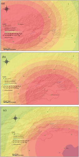
Using EquationEq. (17)(17)
(17) , we calculated the single-station acceptances A(r) of approximately 11 ADTD detectors around Beijing. The distribution maps indicate that the acceptances in areas closer to the detectors are clearly higher and that the acceptances rapidly decrease toward the mountainous areas (see ).
Figure 3. Distributions of the single-station acceptances of the detectors in (a) Zhangjiakou, (b) Guangxiangtai, and (c) Tanggu.
Subsequently, we deduced the ADTD network DE () using the iterative algorithm based on single-station acceptances. According to the recordings of the location modes in the ADTD data detected from 2007 to 2016, these CG lightning strokes were located after their signal sources were received synchronously by 2 to 7 detectors (see for the proportions of each location mode, indicating number of detectors dedicated to locate one lightning flash/stroke). Note that only 11 ADTD detectors in the Beijing region had been selected to estimate the DE for the case study, and thus, the results are only valid in this region. The results indicate that the DEs in the Beijing metropolitan area are relatively higher, almost all are above 60%, and the maximum is 78% (see ).
Figure 4. Deduced CG lightning stroke DE of the ADTD network around Beijing (a) not accounting for the land surface conductivity damping and (b) accounting for the land surface conductivity damping.
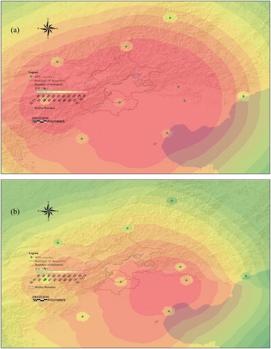
Table 2. Proportions of the ADTD location modes recorded in the lightning location data.
It is reasonable to expect that the CG lightning stroke DEs can reach 60% or higher. Based on a video observation, Idone et al. (Citation1998) found that from 1994 to 1996, the in-site NLDN stroke DEs were most likely between 47% and 67%, while the flash DEs reached between 72% and 86%. Regarding the Vaisala reports, Orville et al. (Citation2011) suggested that the flash DEs of the North American Lightning Detection Network (NALDN) in the contiguous U.S. and southern Canada should surpass 90%, while the overall stroke DEs would be between 60% and 80%.
According to the DE estimates of the ADTD network (), in contrast to the low DEs in the mountainous northern and western regions, the southern plains exhibit a higher DE. Relatively exceptionally low DEs can be found in parts of the Beijing district. These areas are closer to the detector at Guangxiangtai station but far away from the other closest detectors (e.g., Zhangjiakou), meaning that the signal would propagate a long distance over mountains before being received by these detectors; as a consequence, the signal would be attenuated.
We estimated the DEs of the ADTD network by both accounting and not accounting for the damping effects induced by the underlying conductivity. In the comparison of the DEs deduced in the damping and non-damping modes, the DE deduced in the non-damping mode is clearly higher than that in the damping mode, and this discrepancy is exaggerated in mountainous areas (see ), where the lower conductivity leads to a greater attenuation of lightning electromagnetic signals.
4.3. CG lightning stroke density corrected for the deduced DEs
The CG lightning stroke densities (stroke/yr km2) were derived from the ADTD lightning location data. The derivation was performed on the 1 1 km resolution grid, which is 182 km N–S and 181 km E–W and covers the entire Beijing district. The GIS “contain” operator is applied for counting the lightning CG stroke numbers in the grid cells. Then, the CG lightning stroke density Ngrid can be corrected for the grid DEs Fgrid, and the correction formula is
(22)
(22)
where N′grid (stroke/yr km2) is the corrected CG lightning stroke density.
The derivation indicated that the CG lightning stroke densities in the mountainous northern and western regions are clearly lower than that of the other areas (see ). This characteristic is similar to that of the DE estimates. In the mountainous regions, the elevated terrains and low conductivity of the underlying surface, as well as rough and non-flat ground configuration (Li et al. Citation2017), have a strong influence on signal attenuation (Cummins and Murphy Citation2009), which in turn reduces the DE and location accuracy of the ADTD network. However, this result does not convincingly prove that the low CG lightning stroke density in mountainous areas is determined by the low DEs.
Figure 5. Distributions of the ADTD-derived (a) non-corrected CG lightning stroke density and (b) CG lighting stroke density corrected for the DE.
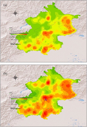
After the CG lightning stroke density was corrected for the DE, the densities in the mountainous northern and western regions increased slightly but remained lower than those of the other areas (see ). Higher densities are still present in the mountainous areas of eastern and southwestern Beijing and in the plains.
A high CG stroke density zone appears in the urban area and its downwind areas (see A in ), in agreement with the hypothesis that an increased urban land-surface roughness could intensify thunderstorm activities (Shepherd et al. Citation2002; Rose et al. Citation2008; Stallins et al. Citation2006; Stallins and Rose Citation2008; Hu et al. Citation2014; Hu Citation2015; Sun and Shu Citation2007).
Additionally, the aerosols serve as cloud condensation nuclei (CCN) and have a substantial effect on cloud properties and the initiation of precipitation (Steiger et al. 2002; Naccarato et al. Citation2003). The higher CG lighting strikes predicted in the plains agree with the hypothesis of the urban aerosol effects on lightning enhancement since the plains usually have more polluted air than the mountainous areas (Tie et al. Citation2015). Moreover, an urban heat island (UHI) can trigger an urban-to-rural thermal circulation and force a convection, which produces enhanced thunderstorms in the metropolitan regions (Jiang and Liu Citation2006; Sun and Shu Citation2007).
Therefore, it is justifiable that the corrected CG lightning stroke densities would be higher in the plains, almost twice (mostly above 2.0 stroke/yr km2) the density in the northern and northwestern areas. Therefore, the urbanization in the plains plays an important role in inducing thunderstorm enhancement that results in a higher CG lightning stroke density without accounting for the higher DEs in the plains.
5. Conclusion
The DE is determined by the LLS performance and sensitivity of the detectors, detector network geometry, and damping factors induced by the underlying land surface conductivity. For this reason, DEs vary due to the underlying land surface and become very low in some regions. This situation leads to a discrepancy between the derived and actual lightning flash/stroke density. This characteristic discounts the applicability of the LLS data. Therefore, we developed an algorithm to estimate DEs which can be used for lightning flash/stroke density correction. The method and its implementation in the CG lightning stroke density correction can be summarized as follows:
It is critical to identify a suitable probability distribution of the LISSs, which is determined for specific regions. In comparison with the lognormal, the Weibull, the extreme value (EV) and the GEV probability distributions, we found that the GEV distribution provides the best fit to the histogram of the sample data.
Based on formula derivations, it was verified that the GEV probability distribution fit would be suitable in estimating the DEs and that the single-station effective radius and acceptance would be determined by the minimum detectable signal strength (Smin).
To address the damping effects induced by the inconsistent underlying land surface conductivity, we estimated the single-station acceptance in the damping modes with respect to the GEV probability distribution of the LISSs.
The DEs of the ADTD network were deduced based on an iterative algorithm using single-station acceptances. According to the LLS location data in Beijing, the number of detectors required to locate the CG lightning strokes was generally between 2 and 7. Thus, the complexity of the iterative algorithm was low, and a convergent solution was found.
The damping effects induced by underlying land surface conductivity were considered in the DE estimates. Thus, the estimate results exhibit that the DEs in the mountains are clearly lower than that in the plains. This finding may be due to the lightning electromagnetic signals propagating over mountainous areas with low-conductivity underlying land surfaces, as well as rough and non-flat ground configuration, which considerably attenuates the signal.
The CG lightning stroke density corrections for the DEs reflected that although the densities in the mountainous northern and western areas increase to some degree, they are still lower than those in the highly urbanized plains. This phenomenon can be related to the increased urban land-surface roughness, the aerosols and the UHI effects on the thermodynamic activity in urban areas.
The DE estimates can be effectively used for correcting the CG lightning flash/stroke density derived from the LLS data. However, we suggest that the location error correction and uncertainty reduction in the lightning detection should be continued by adding new detectors and/or network upgrading and optimizing the network sensor deployment, which would vitally enhance the LLS performance and sensor sensitivity and achieve the goal of DE improvement.
Acknowledgements
This study has been supported by the Climate Change Research Projects of China Meteorological Administration (Project: CCSF201717) and the Research Projects of Institute of Urban Meteorology, CMA (Project: IUMKY201716).
References
- Antonescu B, Burcea S. 2010. A cloud-to-ground lightning climatology for Romania. Mon Weather Rev. 138(2):579.
- Bishop CM. 2006. Pattern recognition and machine learning (information science and statistics). Berlin: Springer-Verlag.
- Bourscheidt V, Cummins KL, Pinto Jr O, Naccarato KP. 2012. Methods to overcome lightning location system performance limitations on spatial and temporal analysis: Brazilian case. J Atmos Ocean Technol. 29(9):1304–1311.
- Changnon SA. 1993. Relationships between thunderstorms and cloud-to-ground lightning in the United States. J Appl Meteor. 32(1):88–105.
- Cummins KL, Murphy MJ. 2009. An overview of lightning locating systems: History, techniques, and data uses, with an in-depth look at the U.S. NLDN. IEEE Trans Electromagn Compat. 51(3):499–518.
- Cummins KL, Murphy MJ, Bardo EA, Hiscox WL, Pyle RB, Pifer AE. 1998. A combined TOA/MDF technology upgrade of the U.S. national lightning detection network. J Geophys Res. 103(D8):9035–9044.
- Drüe C, Hauf T, Finke U, Keyn S, Kreyer O. 2007. Comparison of a SAFIR lightning detection network in northern Germany to the operational BLIDS network. J Geophys Res Atmos. 112(D18114):1–10.
- Etherington TR, Perry GLW. 2017. Spatially adaptive probabilistic computation of a sub-kilometre resolution lightning climatology for New Zealand. Comput Geosci. 98:38–45.
- Evans M, Hastings N, Peacock B. 1993. Statistical distributions, 2nd ed. New York: John Wiley and Sons.
- Fierro AO, Reisner JM. 2011. High-resolution simulation of the electrification and lightning of hurricane Rita during the period of rapid intensification. J Atmos Sci. 68(3):477–494.
- Fierro AO, Mansell ER, Ziegler CL, Macgorman DR. 2011. Application of a lightning data assimilation technique in the WRF-ARW model at cloud-resolving scales for the Tornado outbreak of 24 May 2011. Mon Weather Rev. 140(8):2609–2627.
- Honma N, Suzuki F, Miyake Y, Ishii M, Hidayat S. 1998. Propagation effect on field waveforms in relation to time-of-arrival technique in lightning location. J Geophys Res. 103(D12):14141–14145.
- Hu H. 2015. Spatiotemporal characteristics of rainstorm-induced hazards modified by urbanization in Beijing. J Appl Meteorol Climatol. 54(7):150422143723004.
- Hu H, Wang J, Pan J. 2014. The characteristics of lightning risk and zoning in Beijing simulated by a risk assessment model. Nat Hazards Earth Syst Sci. 14(8):4115–4154.
- Idone VP, Davis DA, Moore PK, Wang Y, Henderson RW, Ries M, Jamason PF. 1998. Performance evaluation of the U.S. National Lightning Detection Network in eastern New York: 2. Location accuracy. J Geophys Res. 103(D8):9057–9069.
- Jiang X, Liu W. 2006. Numerical simulation on impacts of urbanization on heavy rain in Beijing using different land use data. Acta Meteorol Sin. 64(4):527–536 (in Chinese).
- Kotowski A, Kaźmierczak B. 2013. Probabilistic models of maximum precipitation for designing sewerage. J Hydrometeor. 14(6):1958–1965.
- Li D, Rubinstein M, Rachidi F, Diendorfer G, Schulz W, Lu G. 2017. Location accuracy evaluation of ToA-based lightning location systems over mountainous terrain. J Geophys Res Atmos. 122:11,760–11,775. DOI:10.1002/2017JD027520.
- Ma QM. 2015. Technology and fundamentals of lightning monitor. Beijing: Science Press (in Chinese).
- Mäkelä A, Tuomi TJ, Haapalainen J. 2010. A decade of high-latitude lightning location: effects of the evolving location network in Finland. J Geophys Res Atmos.. 115(D21124):1–15.
- Naccarato KP, Pinto Jr O, Pinto IRCA. 2003. Evidence of thermal and aerosol effects on the cloud-to-ground lightning density and polarity over large urban areas of Southeastern Brazil. Geophys Res Lett. 30(13):7–1.
- Naccarato KP, Pinto JO. 2009. Improvements in the detection efficiency model for the Brazilian lightning detection network (BrasilDAT). Atmos Res. 91(2–4):546–563.
- Orville RE, Huffines GR, Burrows WR, Cummins KL. 2011. The North American Lightning Detection Network (NALDN)—Analysis of Flash Data: 2001-09. Mon Weather Rev. 139(5):1305–1322.
- Orville RE, Huffines GR, Burrows WR, Holle RL, Cummins KL. 2002. The North American Lightning Detection Network (NALDN)—First results: 1998–2000. Mon Weather Rev. 130(8):2098–2109.
- Rakov VA, Uman MA. 1990. Some properties of negative cloud-to-ground lightning flashes versus stroke order. J Geophys Res. 95(D5):5447–5453.
- Rose LS, Stallins JA, Bentley ML. 2008. Concurrent cloud-to-ground lightning and precipitation enhancement in the Atlanta, Georgia (United States), Urban Region. Earth Interact. 12(11):1.
- Rudlosky SD, Fuelberg HE. 2010. Pre- and postupgrade distributions of NLDN reported cloud-to-ground lightning characteristics in the contiguous United States. Mon Weather Rev. 138(9):3623–3633.
- Schulz W, Cummins KL, Diendorfer G, Dorninger M. 2005. Cloud-to-ground lightning in Austria: a 10-year study using data from a lightning location system. J Geophys Res Atmos. 110(D09101):1–20.
- Schütte T, Cooray V, Israelsson S. 1988. Recalculation of lightning localization system acceptance using a refined damping model. J Atmos Oceanic Technol. 5:375–380.
- Schütte T, Salka O, Israelsson S. 1987. The use of the Weibull distribution for thunderstorm parameters. J Clim Appl Meteor. 26(4):457–463.
- Shepherd JM, Pierce H, Negri AJ. 2002. Rainfall modification by major urban areas: observations from spaceborne rain radar on the TRMM satellite. J Appl Meteor. 41(7):689–701.
- Stallins JA, Bentley ML, Rose LS. 2006. Cloud-to-ground flash patterns for Atlanta, Georgia (USA) from 1992 to 2003. Clim Res. 30(2):99–112.
- Stallins JA, Rose LS. 2008. Urban lightning: current research, methods, and the geographical perspective. Geogr Compass. 2(3):620–639.
- Steiger SM, Orville RE, Huffines G. 2001. Cloud-to-ground lightning characteristics over Houston, Texas: 1989–2000. J Geophys Res. 107(D11):ACL-1–ACL 2-12.
- Sun JS, Shu WJ. 2007. The effect of urban heat island on winter and summer precipitation in Beijing region. Chin J Atmos Sci. 31(2):311–320 (in Chinese).
- Taszarek M, Czernecki B, Kozioł A. 2015. A cloud-to-ground lightning climatology for Poland. Mon Weather Rev. 143(11):150904101551007.
- Tie X, Zhang Q, He H, Cao J, Han S, Gao Y, Li X, Jia XC. 2015. A budget analysis of the formation of haze in Beijing. Atmos Environ. 100:25–36.
- Williams ER. 2005. Lightning and climate: a review. Atmos Res. 76(1–4):272–287.
- Yao W, Zhang Y, Meng Q, Wang F, Lu W. 2012. A comparison of the characteristics of total and cloud-to-ground lightning activities in hailstorms. Acta Meteorol Sin. 27(2):282–293.