Source analysis of acoustic emissions during granite strain burst

Abstract

The acoustic emission (AE) location technique and fault-plane solution method were used to evaluate the temporal-spatial evolution, released energy variation of micro-cracks, and the difference in b-values for different types of micro-cracks during granite strain burst tests. Results show that AE locations coincide with the macroscopic cracks in the ejection zone. AE locations are scattered for the fracture zone after unloading. The fragment ejection was the results of the combined action of shear, tensile, and compressional micro-cracks; furthermore, the released energy from compressional micro-cracks was largest at the moment of strain burst. Additionally, compressional micro-cracks were the most common, and the tensile micro-cracks were the lease common. For compressional micro-cracks, the overall trend of the b-values was downward, while b-values for shear and tensile micro-cracks both increased. For the fracture zones, the b-value of the micro-cracks was decreased firstly and then increased, while b-values for the ejection zones decreased firstly and then fluctuated and increased.

Keywords:

• Fault-plane solution
• AE location
• event density
• strain burst
• b-value

1. Introduction

Rock burst is a common occurrence along deep mining roadways with high geo-stress environments. In recent years, rock burst phenomena have been investigated using theoretical, numerical, and experimental approaches (Hill et al. 1966; He et al. 2010; Manouchehrian and Cai 2016). Rock bursts are commonly associated with local underground geometry and geology (Ortlepp and Stacey 1994); the most common form of the phenomenon is a strain burst (Hoek et al. 2000).

Conventional research on strain burst mechanisms is based on static rock mechanics. The balance and release of energy during a strain burst was investigated using energy theory (Cook 1963; Salamon 1984), fracture failure theory (Nemat-Nasser and Horii 1982; Mansurov 2001), and damage theory (Xie et al. 2004). Responses to stress redistribution, such as crack propagation, strain energy accumulation, and excavation-induced release of the surrounding rock, are essential issues.

Laboratory tests play a key role in understanding a strain burst, and the damage, splitting, and ejection mechanisms have been explained using true tri-axial unloading strain burst experiments (He 2006). True-triaxial unloading tests can simulate the in-situ stress state and reproduce strain burst phenomenon. Additionally, acoustic emission (AE) technology is an effective method to study the process of fracture evolution for brittle materials. It can monitor the generation and expansion of micro-cracks within brittle materials continuously. Moreover, AE technology is an effective method to study strain burst mechanisms and reveal the AE precursor of strain bursts (He et al. 2010; Gong et al. 2017).

Currently, the study of AE signals during strain burst tests is primarily focused on AE parameters and wave analysis (Sun et al. 2016; Zhao and He 2016). However, a few reports discuss the spatial-temporal evolution of micro-cracks and the cracking mechanism, which was explained using scanning electron microscopy (SEM) images of rock fragments after a strain burst (Tan 1989). AE location technology and fault-plane solution methods were used to study rock mechanics, and fault-plane solutions are a useful quantitative approach for AE source analysis (Sato et al. 1990; Lei et al. 1992; Meglis et al. 1995).

AE locations and fault-plane solution method have been used in uniaxial compression experiments (Sondergeld and Estey 1982; Shah and Labuz 1995), biaxial compression experiments (Kuwahara et al. 1985; Fakhimi et al. 2002), Pseudo-triaxial experiment (Lei et al. 2003; Benson et al. 2008; Graham 2010), and tri-axial compression experiments (Satoh et al. 1986; Ishida et al. 2004). All these experiments have obtained the development of micro-cracks and the sources of rock fracture during the tests. However, the strain burst test is different from the above mentioned experiments, which unloading one direction abruptly after the true tri-axial loading. And the AE locations and fault-plane solution method have seldom used in strain burst simulation tests. Therefore, it is necessary to use the AE locations and fault-plane solution methods to obtain the development of micro-cracks and predict the process of rock failure which is helpful to understand rock burst mechanism better.

The negative slope (b-value) of Gutenberg–Richter (G–R) relation was widely used (as a statistical index) to estimate damage and predict the state of the specimen (Meredith et al. 1990; Lockner 1995; Carpinteri et al. 2012). A large number of experiments have been conducted to study the variation of b-values during the failure procession. Uniaxial compression (Li et al. 1992; Unander 2010), biaxial compression (Chen et al. 2003), and tri-axial compression experiments (Amitrano 2003; Lei et al. 2003) have proved that b-value would drop when the specimen is near failure. However, strain burst (accompanied ejection failure) is a complicated failure mode which is different from uniaxial, biaxial, and tri-axial compression. Hence, the b-value evolution of different types micro-cracks in different failure zones needs to be studied.

In this study, the granite strain burst tests were carried out by self-developed true tri-axial test equipment. Strain burst process is monitored by high speed camera and AE system. Firstly, specimen preparation, loading path, testing system and AE settings were described. Then the methods of AE location and fault-plane solution were introduced. Subsequently, the AE evolution characteristics during strain burst process was investigated. Finally, the spatial-temporal evolution, cracking mechanism, and b-value evolution of micro-cracks were investigated and discussed based on AE results. The aim of this study is to provide some reference for practical engineering design and prevention of strain burst.

2. Experimental procedure granite

2.1. Granite samples

Samples of monzonitic granite were collected from Laizhou, Shandong province in eastern China. The samples are dense and intact with a red meat colour. X-ray diffraction (XRD) analysis reveals the major minerals in the rock are quartz (36.6%), potash feldspar (28.9%), plagioclase (26.7%), and clay minerals (7.8%, kaolinite dominant). Three cylindrical specimens U1, U2, and U3, with nominal dimensions of 50 mm in diameter and 100 mm in length, were prepared for uniaxial compression tests (Table 1). The mean UCS value was 130.79 MPa. Table 1 also shows the P-wave and S-wave velocities of the granite; specifically, the mean P-wave velocity (3551.89 m/s) was used to determine the AE sources.

Table 1. Physical and mechanical properties of Laizhou granite samples.

Sample no.	Density (g/cm^3)	P-Wave velocity (m/s)	S-Wave velocity (m/s)	UCS (MPa)	Young’s modulus (GPa)	Poisson’s ration
U1	2.62	3563.67	2269.33	127.19	35.72	0.27
U2	2.63	3428.52	1857.35	134.23	36.83	0.24
U3	2.63	3663.49	1967.56	130.96	36.47	0.20
Mean	2.63	3551.89	2031.41	130.79	36.34	0.24
SD	0.01	96.29	213.28	2.88	0.57	0.04

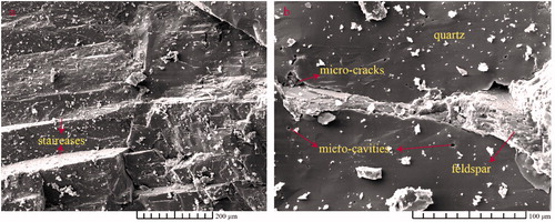
Figure 1 shows two photographs of the micro-scale structure of the granite samples obtained from SEM imagery. Staircase-shaped feldspar crystals are present (Figure 1a), and micro-cavities and cracks are present in the contact zone between quartz and feldspar crystals (Figure 1b). Minerals with different hardness along contact zones, micro-cavities, and cracks contribute to rock heterogeneity. The underlying causes of initiation and propagation of micro-cracks are the microscopic material and structural properties (Liu et al. 2004).

Figure 1. SEM photos of the Laizhou granite sample; (a) staircase-formed feldspar crystals and (b) micro-cavities and cracks exist in the contact zone between the quartz and feldspar.

2.2. Strain-burst test and AE settings

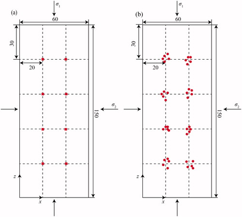
Granite blocks were machined into rectangular prism specimens approximately 150 mm in length, 60 mm in width, and 30 mm in thickness. Table 2 shows the experimental scheme of the three strain-burst tests. The initial stress state is determined using the geo-stress regression formula at the sampling area, which is approximately σ₁ = 35.5 MPa, σ₂ = 33.1 MPa, and σ₃ = 19.8 MPa for granite at 1000 m depth (Sun and Tan 1995).

Table 2. Experiment scheme and failure information.

Specimen	Dimension (mm*mm*mm)	Initial stress state (MPa)	Failure stress state (MPa)			Stress drop for σ1 (MPa)	Dimension* of burst pit (mm*mm*mm)
			σ1	σ2	σ3
G1	149.98*60.16*30.02	σ1=35.5 σ2=33.1 σ3=19.8	189.2	34.5	0.0	159.2	60*32*18
G2	150.02*60.09*30.02		184.4	33.8	0.0	153.2	60*55*18
G3	150.02*60.06*30.00		205.5	34.0	0.0	165.3	60*48*18

* Note: the dimension is the largest length of burst pit in each direction.

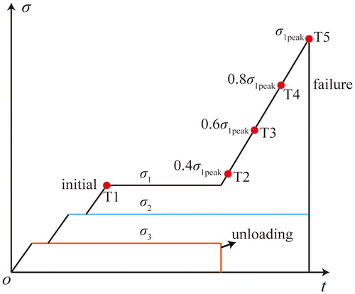
The stress path of the strain burst was divided into five parts (oa, ab, bc, cd, and de) (Figure 2). The critical points for T1 through T5 were the initial stress state at 40%, 60%, 80%, and 100% of the maximum σ₁, respectively. Stage oa is the initial loading stage, where the initial stresses were loaded gradually, and each level was held for a period to make the stress distributed uniformly. In stage ab, σ₃ was unloaded abruptly while σ₁ was loaded at a constant rate (0.25 MPa/s) to simulate stress concentration. Stages bc, cd, and de contained all the damage, and de was the strain burst stage.

Figure 2. Stress path of strain burst.

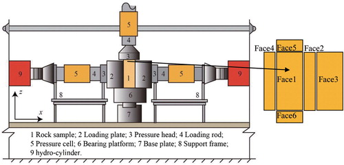
A modified true tri-axial apparatus was applied to our tests (Figure 3) (He et al. 2010). The specimen had six faces, and the orientation of ‘Face 1’ was in the positive y-axis direction as well as the unloading face. Tri-axial homogeneous stresses (σ₁ ≥ σ₂ ≥ σ₃) could be applied independently in the three mutually perpendicular directions. The horizontal loading rod representing σ₃ was detachable and could be removed quickly to mimic unloading on one face of the specimen. Loading plates on the other faces were held constant. Initial stresses were applied in a step-by-step manner, and each level was held constant for approximately 5 minutes to ensure a uniform stress distribution. When the initial stress state was applied for some minutes, σ₃ was unloaded abruptly, and σ₁ was increased to simulate stress concentration until a strain burst occurred.

Figure 3. Schematic of strain burst machine.

The PCI-2 system produced by the American Physical Acoustics Corporation (PAC) was used for AE monitoring. This system uses an 18-bit A/D switching technology that allows instantaneous time-waveform recording. In this study, AE signals were amplified to 40 dB, and the threshold, sampling frequency, and sampling length were set to 40 dB, 5 MHz, and 4096, respectively.

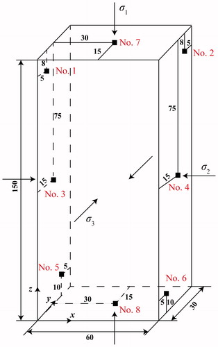
Eight Nano30 sensors with a response frequency of 100-400 kHz were used to acquire the AE signals (Figure 4). Six sensors (No. 1 to No. 6) were placed in the σ₂ direction. On the left side of the specimen, three sensors (No. 1, No. 3, and No. 5) were arranged on the diagonal of the specimen, and on the opposite face, another three sensors (No. 2, No. 4, and No. 6) were attached on the anti-diagonal. The No. 7 and No. 8 sensors were placed on the centre of the top and bottom faces of the specimen. All sensors were equipped with a 2/4/6 pre-amplifier. During testing, petroleum jelly was applied to the sensors to ensure good contact. Additionally, sensors were fixed on the cavities of the plate by a spring and antifriction plastic sheet, which was placed in the interface between the sensor and cavity.

Figure 4. Arrangement of AE sensors (unit: mm).

2.3. Location precision tests

Before loading, pencil-lead break tests were processed on the front face (Face 1) of the specimen to ensure location precision. The front face of the specimen was divided into 15 zones (Figure 5a), and the intersections (a total of 8) of the dotted lines mark all pencil-lead break positions. The tests were conducted 5 times for each point, and the mean value of the coordinates are in accordance with the hit position, which suggests that the precision (less than 15% of thickness) of the location meets the requirement for the temporal-spatial evolution of the micro-cracks (Figure 5b).

Figure 5. Pencil-lead breakage test and results (unit: mm), (a) pencil-lead break position and (b) location results.

3. AE location and fault-plane solution

3.1. Iterative location

The iterative localization algorithm used in this study is the most common method for 3D AE location. In this location method, the arrival time of each sensor is measured and used as the reference value for a calculated arrival time, which is computed from a trial location. The trial location is corrected using the residuals between the measured and calculated arrival time.

In this study, eight sensors were used, and the over-determined system had to ensure that the residuals for each sensor were minimized. In addition, convergence criteria could be set to terminate at a specific iteration according to the desired accuracy (Grosse and Ohtsu 2008).

3.2. Fault-plane solution method

The fault-plane solution method was commonly used in source mechanism studies in rock specimens and was introduced from earthquake seismology (Sondergeld and Estey 1982; Kuwahara et al. 1985; Zang et al. 1998). This method uses polarities and ray directions of the P-wave to constrain possible double-couple fault-plane solutions. For a located AE event, the polarity value pol was calculated by (1) $$\mathit{pol}=\frac{1}{k}\sum _{i=1}^k\mathit{sign}\left(A^i\right)$$(1)

Where k is the number of sensors which received the same event, and A is the first motion amplitudes. The polarity is used to separate type-S (shear) events (−0.25≤ pol ≤ 0.25) from type-T (tensile) (−1≤ pol < −0.25) and type-C (compression) sources (0.25≤ pol ≤ 1).

3.3. Determination of the first motion amplitude of the P-wave

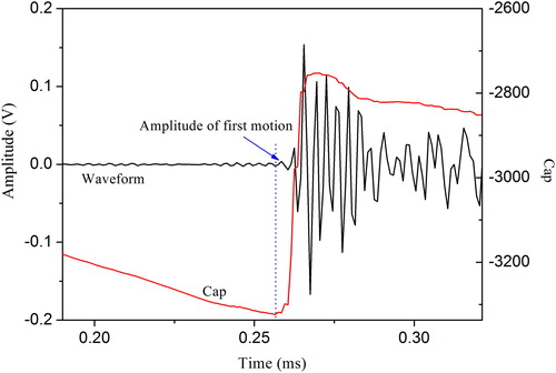
Determination of A(x) requires the P-wave onset times of the AE waveform. The exact onset is determined by calculating the Akaike information criterion (AIC) function directly from the signal (Katsuyama 1996). For an AE waveform during the granite strain burst test (Figure 6), the time series of n (n = 4096) data were divided into two portions, one with k number of points, and another with n−k points. For each value of k (k = 1, 2, …, 4096), the AR model for the k and n−k data was established, and the AIC was adopted to estimate the rationality of the models. The criterion C_ap is expressed as follows (Katsuyama 1996; Liu et al. 2015): (2) $${\mathrm{C}}_{\text{ap}}=\mathit{AI}{C}_1+\mathit{AI}{C}_2=k\hspace{0.17em}\text{log}\hspace{0.17em}{\delta }_1^2+(n-k)\hspace{0.17em}\text{log}\hspace{0.17em}{\delta }_2^2+n(\hspace{0.17em}\text{log}\hspace{0.17em}2\pi +1)+12$$(2) where δ₁ and δ₂ are the variances of the AR model of the k data and n−k data, respectively. The values of C_ap of each k from 1 to 4096 are calculated, and the time of the minimum value of C_ap can be observed as the P-wave onset time, (Figure 6). The minimum C_ap, which is represented by the dashed line, denotes the onset time of the signal, and the next waveform is the amplitude of the first motion.

Figure 6. Schematic of the P-wave onset time and amplitude of the first motion determination.

4. Results and discussion

4.1. Failure process of granite strain burst

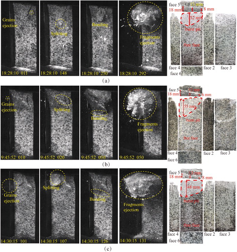
Strain burst loading paths for specimens G1, G2, and G3 were recorded (Figure 2), and the stress drops accompanying the strain burst were 159.2 MPa, 153.2 MPa, and 165.3 MPa for G1, G2, and G3, respectively. Additionally, Figure 7 shows the fragment ejection and images of the specimen after failure. The strain burst typical process includes grain ejection, fragment splitting, bending of the sample and rock fragment ejection. Furthermore, obvious burst pits were located in the upper side of the specimen, but burst pit dimensions were different for the three specimens. The volume of the burst pit for specimen G3 was largest. Moreover, the fracture after ejection was an inclined plane viewed from ‘face 5’, and the burst pit depths for the three specimens were same (18 mm). Furthermore, the cracks could be observed on ‘face 2’ and ‘face 4’, and the orientation of those cracks was similar that perpendicular to the free face (‘face 1’) approximately.

Figure 7. Failure process and photos of granite strain burst for specimen (a) G1, (b) G2, and (c) G3, respectively, the number in the bottom left corner of the photos is the physical time of the corresponding phenomena.

4.2. Spatial distribution of AE events

The spatial distribution of AE events was presented as hypocentre density contours on ‘face 4’. Figure 8 shows the non-accumulated event density contours for different key points (T1–T5) and also contains the corresponding photo of specimen G1 after failure. Additionally, failure zones on ‘face 4’ were divided into two zones, an ejection zone and fracture zone. The shapes of the ejection and fracture zones both were rectangular, and the length and width of the rectangle were determined using the actual damage dimension.

Figure 8. (a–e) Event density contours for T1–T5, respectively, and (f) failure photos of specimen G1. Note: events of each point were non-accumulated, for example, events of point T2 were events occurred from T1 to T2.

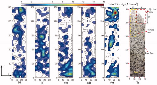
During the initial loading stage (point T1) for specimen G1, the maximum event density was approximately 9.3 AE·mm⁻³, and it was located in the upper side (z = 140 mm) of the specimen, additionally, in the middle-upper part (z = 105mm) and bottom of the specimen both had a concentration of AE events. After unloading (point T2), the new AE events centralized gradually to the middle of the specimen and focused on two position with z-axis coordinates of 85 mm and 45 mm. When the maximum principal stress increased to 60% (point T3) and 80% (point T4) of peak stress, new AE events were concentrated on the bottom (z = [8, 25 mm]) and top (z = [135, 145 mm]) of the specimen. The maximum event density was also located on the bottom (z = 8 mm) of the specimen. For the strain burst moment (point T5), the ejection zone corresponds to the maximum number of AE events. In addition, the middle (z = [60, 90 mm]) and bottom (z = [5, 25 mm]) of the specimen both contained concentrations of AE events.

For specimen G1, Figure 9(a) shows the variation in maximum event density for the key points and also contains the unloading moment. Figure 9(b and c) show the variation of accumulated percentage of events and the corresponding stress paths, respectively. Additionally, Table 3 lists the specific values for maximum event density and event percentage for the three samples. Maximum event density trends were similar, and the unloading point corresponded the minimum stress and the failure point corresponded to the largest stress value. After unloading, the maximum event density first increased, then decreased and then increased again.

Figure 9. (a) Maximum event density, (b) percentage of events number to total events and (c) three principal stress versus time for specimen G1.

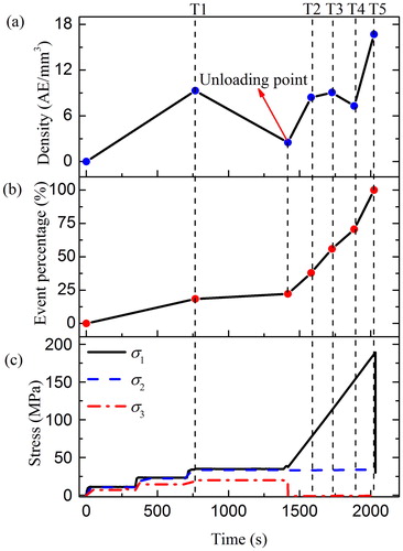
Table 3. Variation of maximum event density and accumulated event percentage for granite strain burst.

Specimen	Maximum event density (AE/mm^3)						Accumulated event percentage (%)
	T1	Unloading	T2	T3	T4	T5	T1	Unloading	T2	T3	T4	T5
G1	9.3	2.5	8.4	9.1	7.3	16.7	18.4	22.1	37.9	55.9	70.6	100
G2	15.9	4.0	12.9	5.0	16.1	19.9	16.0	18.4	23.7	49.8	77.2	100
G3	7.0	3.8	10.9	4.9	32.9	37.6	12.8	23.3	25.3	30.8	61.6	100

The event density contours for five different key points in specimen G2 and G3 were similar with key points from specimen G1. AE gathering sites, which occurred during the initial loading process, were distributed between three different positions in the specimen. Additionally, after unloading (point T2), the development of new AE events in specimens G2 and G3 was more scattered. Furthermore, during stress concentration (points T3 and T4), the number of new AE events decreased (T3) first and increased later (T4). At the moment of strain burst, the position of maximum density in both specimens G2 and G3 were located in the ejection zone, which was similar to specimen G1.

The percentages of AE events during initial loading were approximately 18.4%, 16.0%, and 12.8% for specimens G1, G2, and G3, respectively. There were a few new events caused by the unloading that account for approximately 3.7%, 2.4%, and 10.5% for the above three samples. After unloading, the number of AE events increased with increasing maximum principal stress. Additionally, the increments of AE events in the last stage (T4–T5) were largest and accounted for approximately 29.4%, 22.8%, and 38.4% for specimens G1, G2, and G3, respectively.

4.3. Spatial distribution of three types of micro-cracks

AE events can be regarded as micro-cracks in a specimen, and according to the fault plane solution method, these micro-cracks can be divided into three types. Figure 10 shows the spatial and temporal distribution of the shear, tensile, and compressional micro-cracks for specimen G1, and Table 4 lists the number and percentage of the three types of micro-cracks.

Figure 10. Spatial distribution of three types of micro-cracks for specimen G1, (a–e) for T1–T5, respectively.

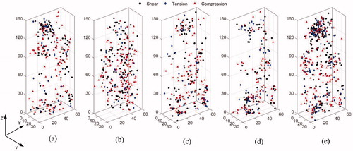
Table 4. Number and ratio of the three types of micro-cracks.

Specimen	Type-S number	Type-T number	Type-C number	Total number of micro-cracks	Ratio of Type-S (%)	Ratio of Type-T (%)	Ratio of Type-C (%)
G1	546	258	614	1418	38.5	18.2	43.3
G2	453	193	590	1236	36.7	15.6	47.7
G3	672	330	679	1681	40.0	19.6	40.4

Compressional micro-cracks are the most abundant in the specimens. Shear micro-cracks are present in a moderate amount, and tensile micro-cracks are a minimal proportion. For specimens G1, G2, and G3, the ratios of shear micro-cracks were 38.5%, 36.7%, and 40.0%, respectively, and the ratios of tensile micro-cracks were 18.2%, 15.6%, and 19.6%, respectively. In short, for strain burst testing, shear micro-cracks accounted for more than 35% of all micro-cracks. The tensile micro-cracks accounted for less than 20%, and mixed-mode micro-cracks comprised more than 40%.

During the initial loading stage, the most of shear micro-cracks are distributed in the upper left corner of specimen while tensile and compressional micro-cracks were more scattered (Figure 10). After unloading, the distribution of shear and compressional micro-cracks was similar in that both were scattered inside the specimen. Additionally, a few micro-cracks formed the top and bottom of the specimens. During stress concentration, micro-cracks centralized gradually in some local zones. When the maximum principal stress was increased to 60% and 80% of peak stress, shear and tensile micro-cracks concentrated in the bottom right corner and bottom left zone, respectively. However, compressional micro-cracks both concentrated in the middle and bottom of the specimens during the above two stages. For the strain burst stage, the three types micro-cracks all concentrated in the top and bottom left corner of the sample. The top left corner corresponds to the ejection zone. Furthermore, some compressional micro-cracks were located in the middle and left side of the specimens.

Figure 11 shows the maximum principal stress versus time and the accumulation and release of AE energy for specimen G1. The energy was taken as the average of the values received from each sensor. At the unloading moment, the released energy in shear and compressional micro-cracks both suddenly increased. Compressional cracks released more energy than shear cracks. During stress concentration, the amplitude of energy variations for the three types micro-cracks were all smaller. However, when the strain burst, the energy increment of the compression micro-cracks was largest and the energy released by the shear micro-cracks was smaller.

Figure 11. (a) evolution of accumulated energy for three types of micro-cracks with time elapses and (b) stress paths for specimen G1.

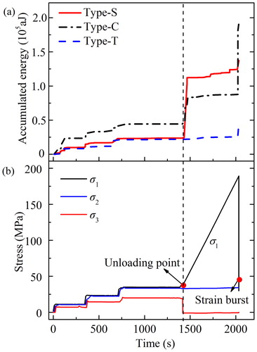
Table 5 lists the energy increments of the three types of micro-cracks at unloading as well as strain burst moments for three samples. At the moment of unloading, the energy released by the shear micro-cracks was largest. However, the released energy from compressional micro-cracks was largest at the moment of strain burst. Additionally, at this moment, the energy released by shear and tensile micro-cracks were equal approximately. Therefore, for unloading, the shear effect was dominant while compression was predominant stress in strain burst.

Table 5. Energy increment of three types of micro-cracks at unloading and strain burst moments.

Specimen	Energy increment for unloading (10^5aJ)			Energy increment for strain burst (10^5aJ)
	Type-S	Type-T	Type-C	Type-S	Type-T	Type-C
G1	0.88	0.02	0.28	0.11	0.10	0.86
G2	0.57	0.06	0.33	0.16	0.13	0.80
G3	0.65	0.05	0.30	0.15	0.16	0.77

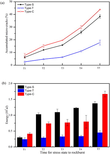
Figure 12 shows the mean accumulated percentage for the three types of micro-cracks and released AE energy in different stages for three granite samples. The total number of micro-cracks was 1418, 1236, and 1681 for specimen G1, G2, and G3, respectively. The percentages of shear and compressional micro-cracks were similar; furthermore, the specific percentage values of shear micro-cracks were slightly lower than values for compressional micro-cracks. Values for tensile micro-cracks were the smallest of the three types (Figure 12). The growth rate of tensile micro-cracks was the lowest. Additionally, increments of mean AE energy from the three types’ micro-cracks, accumulated from unloading to strain burst, were all minor. However, for the strain burst moment, the energy of each type micro-cracks all increased, and the increment of compressional micro-cracks was largest.

Figure 12. The mean accumulated (a) percentage of the three types of micro-cracks and (b) released AE energy of five key points (T1–T5) for three samples.

4.4. Evolution of b-values

The Gutenberg-Richter frequency-magnitude relationship for earthquake population was used to observe AE amplitude distributions (Mogi 2006). AE amplitudes increased before failure which is documented by a drop in negative slope (b-value) of cumulative amplitude-frequency distributions (Lockner et al. 1991). In this study, due to eight sensors used, the average focal amplitude is calculated as (Zang et al. 1998). (1) $$\overline{A}=\sqrt{\frac{1}{n}\sum _{i=1}^n{\left(\frac{r_i}{10}{A}_i\right)}^2}$$(1)

Where n is the number of channels which receive the same AE signal, n is from 4 to 8, r_i is the hypocentre distance to the corresponding sensor, A_i is the focal amplitude of the AE wave received by sensor i. Because the distances between the hypocentre and sensors are different, the amplitude A_i was adjusted to the equivalent event amplitude ($\frac{r_i}{10}{A}_i$) at a distance of 10 mm from the hypocentre.

4.4.1. Evolution of b-values for micro-cracks

Figure 13(a) shows the variation of the mean b-value for the total micro-cracks during granite strain burst tests. With the time elapse, b-value increases firstly and then decrease. According to the definition of b-value, it can be known that a small b-value corresponds to an increase in the proportion of large scale micro-cracks, and vice versa, a large b-value indicates that number of small scale micro-cracks is increase. From T1 to T2, the b-value increases, which means that the proportion of small scale events increases. However, from T2 to T3, the b-value decreases, which means that the proportion of large scale events increases, i.e. large-scale micro-cracks increases. Additionally, from T3 to T4, the changes of b-value is small which represents stable expansion. In the end, at the moment of strain burst (T5), the b-value decreases, representing the penetration of micro-cracks which is similar with the exist study (He et al. 2015).

Figure 13. Evolution of mean b-values of micro-cracks in different key points for three samples, (a) for total micro-cracks (b) compression, (c) shear and (d) tensile micro-cracks.

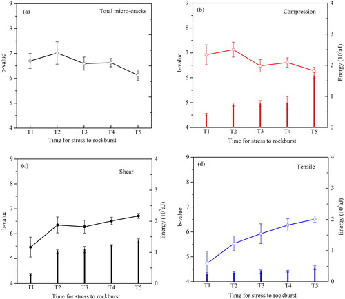
Figure 13(b–d) shows the variation of the mean b-values for the three micro-cracks during granite strain burst tests also gives the corresponding accumulated AE energy at five key points. For the compressional micro-cracks, the overall trend of b-values was downward, while b-values of shear and tensile micro-cracks were both generally increasing. The variation trend of the compressional micro-crack is the same as that for total micro-cracks. The b-value variation of shear, tensile and total micro-cracks is different. It is shown that compression micro-crack plays an important role in b-value variation, because the compressional micro-cracks occupy the highest proportion of energy during the process of strain burst.

4.4.2. Evolution of b-values for different zones

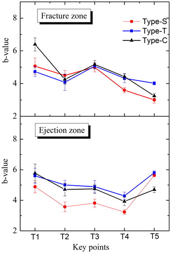
Figure 14 shows the variation of the b-values of three types micro-cracks during granite strain burst tests for the fracture and ejection zones that defined in Figure 8. For the fracture zone, the evolution of the b-value of the micro-cracks was decreased firstly and then increased and decreased to the minimal value in the end. However, the evolution of the b-value for ejection zone was different with the fracture zone that decreased firstly and then fluctuated and increased when strain burst occurred. The decrease of the b-value means the increase of the ratio of the large scale micro-cracks, i.e. the increase of the b-value means the small scale micro-cracks is domain. Therefore, in the ejection zone, the fragments ejection was caused by the accumulation of the small scale micro-cracks.

Figure 14. Evolution of mean b-values of micro-cracks in different zones.

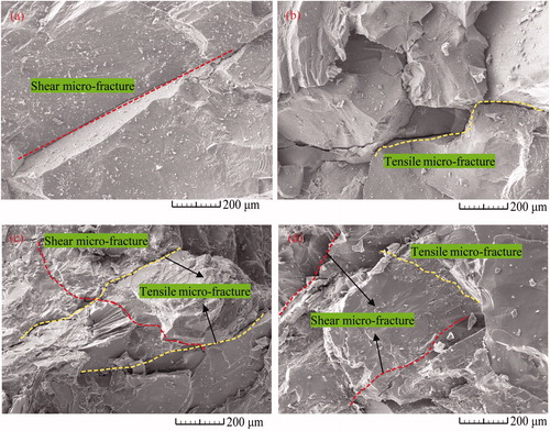
In order to verify micro fractures in fragments from the fracture and ejection zones, rock fragments from the above zones were collected and examined using an SEM (images were magnified 200 times). Figure 15 shows the state of the micro fractures. The number of micro fractures in the ejection zone was more than the number of micro fractures in the fracture zone; however, the scale of the micro fractures in fracture zone was larger. Moreover, micro fractures in the ejection fragments had obvious flaked features. Therefore, at the moment of strain burst, the accumulation of many shear and tensile micro-cracks lead to block ejection. Micro-crack penetration caused the final failure of the specimens.

Figure 15. SEM photos of the fragments which taken from (a–b) fracture zone to (c–d) ejection zone.

5. Conclusions

In this article, the fault-plane solution method was used to analyse granite strain burst AE location results. We examined the temporal-spatial evolution of micro-cracks, variation of three types of micro-cracks, released energy evolution process in different stages, and the difference in b-values for different types of micro-cracks and different zones. Specific conclusions are listed as follows:

1. AE locations are consistent with the macroscopic failure for the ejection zone, while AE locations are more scattered for the fracture zone after unloading.

2. The ejected fragments were the result of the combined action of the shear, tensile, and compressional micro-cracks; furthermore, the released energy from compressional micro-cracks was largest at the moment of strain burst.

3. Compressional micro-cracks made up the largest proportion of micro-cracks, shear micro-cracks were secondary, and the tensile micro-cracks make up the smallest proportion. In short, for the strain burst test, the shear micro-cracks accounted for more than 35% of all micro-cracks, the tensile micro-cracks accounted for less than 20%, and mixed-mode micro-cracks comprised more than 40%.

4. For the total and compressional micro-cracks, the overall trend of the b-values was downward, while b-values for shear and tensile micro-cracks both increased generally. For the fracture zones, the b-value of the micro-cracks was decreased firstly and then increased, while b-values for the ejection zones decreased firstly and then fluctuated and increased.

Disclosure statement

No potential conflict of interest was reported by the author(s).

Additional information

Funding

Financial support from the National Key Research and Development Program (Grant No. 2016YFC0600901) and National Natural Science Foundation of China (Grant No. 51704298) are gratefully acknowledged.

References

- Amitrano D. 2003. Brittle-ductile transition and associated seismicity: experimental and numerical studies and relationship with the b value. J Geophys Res Solid Earth. 108(B1):2044.
- Benson PM, Vinciguerra S, Meredith PG, Young RP. 2008. Laboratory simulation of volcano seismicity. Science. 322(5899):249–252.
- Carpinteri A, Corrado M, Lacidogna G. 2012. Three different approaches for damage domain characterization in disordered materials: fractal energy density, b-value statistics, renormalization group theory. Mech Mater. 53:15–28.
- Chen SC, Zhaoyong XU, Runhai Y, Jinming Z. 2003. Features of acoustic emission during fracturing process of granite block with v-shaped structure under biaxial compression. Seismol Geol. 25(2):317–326. (in Chinese)
- Cook NGW. 1963. The basic mechanics of rockbursts. J South Afr Inst Min Metall. 64:71–81.
- Fakhimi A, Carvalho F, Ishida T, Labuz JF. 2002. Simulation of failure around a circular opening in rock. Int J Rock Mech Min Sci. 39(4):507–515.
- Gong Y, Song Z, He M, Gong W, Ren F. 2017. Precursory waves and eigenfrequencies identified from acoustic emission data based on singular spectrum analysis and laboratory rock-burst experiments. Int J Rock Mech Min Sci. 91:155–169.
- Grosse C, Ohtsu M. 2008. Acoustic emission testing. Berlin, Germany: Springer Berlin Heidelberg.
- Graham CC. 2010. Comparison of polarity and moment tensor inversion methods for source analysis of acoustic emission data. Int J Rock Mech Min Sci. 47(1):161–169.
- He M. 2006. Rock mechanics and hazard control in deep mining engineering in China. Proceedings of the 4th Asian Rock Mechanics Symposium. Singapore: World Scientific Publishing Co., Ltd.
- He M, Miao J, Feng J. 2010. Rock burst process of limestone and its acoustic emission characteristics under true-triaxial unloading conditions. Int J Rock Mech Min Sci. 47(2):286–298.
- He M, Zhao F, Cai M, Du S. 2015. A novel experimental technique to simulate pillar burst in laboratory. Rock Mech Rock Eng. 48(5):1833–1848.
- Hill FG, Cook NGW, Hoek E, Ortlepp WD, Salamon MDG. 1966. Rock mechanics applied to study of rockbursts. Johannesburg: South African Institute of Mining and Metallurgy.
- Hoek E, Kaiser P, Bawden WF. 2000. Support of underground excavations in hard rock. In E. Hoek, P. K. Kaiser, W. F. Bawden, editors. Dimensionnement. Boca Raton, FL: CRC Press.
- Ishida T, Chen Q, Mizuta Y, Roegiers J-C. 2004. Influence of fluid viscosity on the hydraulic fracturing mechanism. J Energy Resour Technol. 126(3):190–200.
- Katsuyama K. 1996. Application of AE techniques. Translated by Feng XT. Beijing:Metallurgy Industry Press.
- Kuwahara Y, Kyamamoto, M. Kosuga I, Hirasawa T. 1985. Focal mechanisms of acoustic emissions in abukuma-granite under uniaxial and biaxial compressions. Science Reports of the Tohoku University Fifth, p. 30.
- Lei X, Nishizawa O, Kusunose K, Satoh T. 1992. Fractal structure of the hypocenter distributions and focal mechanism solutions of acoustic emission in two granites of different grain sizes. J Phys Earth. 40(6):617–634.
- Lei X, Kusunose K, Satoh T, Nishizawa O. 2003. The hierarchical rupture process of a fault: an experimental study. Phys Earth Planet Inter. 137(1–4):213–228.
- Li H, Yin X, Li S, Li J. 1992. The experimental research on b value of ae for the rock specimens with pre-existing crack or notch under uniaxial compression. Acta Seismol Sin. 5(4):867–875.
- Liu HY, Roquete M, Kou SQ, Lindqvist PA. 2004. Characterization of rock heterogeneity and numerical verification. Eng Geol. 72(1–2):89–119.
- Liu J-P, Li Y-h, Xu S-D, Xu S, Jin C-y, Liu Z-S. 2015. Moment tensor analysis of acoustic emission for cracking mechanisms in rock with a pre-cut circular hole under uniaxial compression. Eng Fract Mech. 135:206–218.
- Lockner DA. 1995. Rock failure. Washington, D.C.: American Geophysical Union.
- Lockner DA, Byerlee JD, Kuksenko V, Ponomarev A. 1991. Observations of quasistatic fault growth and shear fracture energy in granite. Nature. 350:39–42.
- Manouchehrian A, Cai M. 2016. Simulation of unstable rock failure under unloading conditions. Can Geotech J. 53(4):150617143612000.
- Mansurov VA. 2001. Prediction of rockbursts by analysis of induced seismicity data. Int J Rock Mech Min Sci. 38(6):893–901.
- Meglis IL, Chows TM, Young RP. 1995. Progressive microcrack development in tests in Lac du Bonnet granite—I. Acoustic emission source location and velocity measurements. Int J Rock Mech Min Sci. 32(8):741–750.
- Meredith PG, Main IG, Jones C. 1990. Temporal variations in seismicity during quasi-static and dynamic rock failure. Tectonophysics. 175(1–3):249–268.
- Mogi K. 2006. Experimental rock mechanics. London: Taylor & Francis.
- Nemat-Nasser S, Horii H. 1982. Compression‐induced nonplanar crack extension with application to splitting, exfoliation, and rockburst. J Geophys Res. 87(B8):6805–6821.
- Ortlepp W, Stacey T. 1994. Rockburst mechanisms in tunnels and shafts. Tunn Undergr Sp Tech. 9(1):59–65.
- Salamon MDG. 1984. Energy considerations in rock mechanics: fundamental results. J S Afr I Min Metall. 84(8):233–246.
- Sato T, Nishizawa O, Kusunose K. 1990. Fault development in Oshima granite under triaxial compression inferred from hypocenter distribution and focal mechanism of acoustic emission. Sci Rep Tohoku Univ. 33:241–250.
- Satoh T, Idehara O, Nishizawa O, Kusunose K. 1986. Hypocenter distribution and focal mechanisms of AE events under triaxial compression: focal mechanisms of AE Events in Yugawara Andesite. 39(3):351–360.
- Sondergeld CH, Estey LH. 1982. Source mechanisms and microfracturing during uniaxial cycling of rock. PAGEOPH. 120(1):151–166.
- Shah KR, Labuz JF. 1995. Damage mechanisms in stressed rock from acoustic emission. J Geophys Res. 100(B8):15527–15539.
- Sun XM, Xu HC, Zheng LG, He MC, Gong WL. 2016. An experimental investigation on acoustic emission characteristics of sandstone rockburst with different moisture contents. Sci China Technol Sci. 59(10):1549–1558.
- Sun Y, Tan CX. 1995. An analysis of present-day regional tectonic stress field and crustal movement trend in China. J Geomech. 1(3):1–12. (in Chinese)
- Tan Y. 1989. Analysis of fractured face of rockburst with scanning electron microscope and its progressive failure process. J Chin Electr Microsc Soc. 8(2):41–48. (in Chinese)
- Unander TE. 2010. Analysis of acoustic emission waveforms in rock. Res Nondestruct Eval. (3):119–148.
- Xie H, Peng R, Yang J. 2004. Energy dissipation of rock deformation and fracture. Chin J Rock Mech Eng. 23(21):3565–3570. (in chinese)
- Zang A, Wagner FC, Stanchits S, Dresen G, Andresen R, Haidekker MA. 1998. Source analysis of acoustic emissions in Aue granite cores under symmetric and asymmetric compressive loads. Geophys J Royal Astron Soc. 135(3):1113–1130.
- Zhao F, He MC. 2016. Size effects on granite behavior under unloading rockburst test. Bull Eng Geol Environ. 76:1183–1197.