Comparative study of the possible lower ionospheric anomalies in very low frequency (VLF) signal during Honshu, 2011 and Nepal, 2015 earthquakes

Abstract

We present perturbations in very low frequency (VLF) signals received at Ionospheric & Earthquake Research Centre (IERC) (Lat. 22.50${}^{°}$N, Long. 87.48${}^{°}$E) during and prior to two earthquakes, one on 11 March 2011 at 11:16:24 LT (M = 9) in Honshu, Japan and another on 12 May 2015 at 12:35:19 LT (M = 7.3) in Kodari, Nepal. The VLF signal transmitted from JJI (22.2 kHz) in Japan (Lat. 32.05${}^{°}$N, Long. 131.51${}^{°}$E) showed strong shift in VLF-sunrise terminator times towards night-time few days prior to both the earthquakes. These two earthquakes took place near the transmitter JJI and receiver IERC respectively. We simulated the VLF sunrise terminator time shifts using the long wavelength propagation capability (LWPC) code. To effectively represent the D-region ionospheric variabilities, we assumed a mean dynamic perturbation over the path and presented them with a set of effective Wait’s parameters (β_eff, $h_{\mathit{eff}}^{\prime }$). We have successfully reproduced the temporal trend of the normalized VLF signal amplitude at VLF sunrise terminators for a few days around both the earthquakes. We used Wait’s exponential model for estimating the altitude profile of D-region electron density ($N_e(h)$) at VLF sunrise terminator times around both the earthquakes and quantified the changes of those $N_e(h)$ profiles.

Keywords:

• Earthquake
• VLF
• terminator shift
• modeling
• LWPC

1. Introduction

Earthquake is a very complex and multi-parametric physical process that involves a wide range of crustal movement from microscopic to macroscopic scale. The generation mechanism of earthquake and its outbursts are well connected with several geo-chemical and geo-physical processes which are also interlinked. Scientific community has proposed numerous methods to study the pre-seismic phenomena but there is significant dearth of successful prediction. In 1960s, a new idea came up to identify the seismic mechanism where instead of study of solid earth, its atmosphere was thought to be the useful tool. Solar and Cosmic rays are the main sources of ionization of the earth’s ionosphere and its variabilities. In this new thought of seismic mechanism, earthquake was treated as a source of direct and indirect ionization. Starting from the ground surface and lithosphere, it is believed that earthquake mechanism techniques can couple the lithosphere, atmosphere and ionosphere via various channels, such as (a) thermal, (b) chemical, (c) acoustics and (d) electromagnetic channels (Pulinets and Boyarchuk 2004; Molchanov 2009; Pulinets and Ouzounov 2011). This mechanism plays the key role to study the pre-seismic phenomena and is commonly known as the Lithospheric-Atmospheric-Ionospheric Coupling (LAIC) mechanism (Pulinets and Ouzonov 2011).

LAIC contains several modelling approaches for various channels. For the coupling through acoustic channel, Atmospheric Gravity Wave (AGW) generates several days before the earthquake and propagates along the upward direction (Korepanov et al. 2009). During seismo-gravitational vibrations, the Earth’s surface can affect the atmosphere as a piston and can cause variations in temperature, conductivity and pressure resulting in AGW generation in the atmosphere. Movements of the Earth’s crust, unstable thermal anomalies and unstable release of lithospheric gases into the atmosphere (Gokhberg et al. 1996) can be the leading factors to generate the AGW which in turn perturb the ionospheric plasma neutral component and charged particle density. Several models were proposed with variety of approaches starting from seismo-gravitation vibrations which generates waves with periods of 30 minutes to 4 hours during seismological measurements (Lin’kov et al. 1990). Pressure of atmospheric gases due to pre-seismic Joule heating (Hegai et al. 2006), AGW Spectrum Full-Wave Model (SFWM) (Hickey et al. 2009), neutral atmosphere-ionosphere-coupling (Longnonne 2010), Radar and Digisonde observation and normal modes summation techniques (Hegai et al. 2006) etc. are the significant model approaches of this study. Electric field modulation is the major source of electromagnetic channel which is caused due to the emission of radioactive gases (Pulinets 1998; Pulinets et al. 2000; Pulinets and Boyarchuk 2004; Pulinets and Liu 2004; Pulinets et al. 2006). Radon causes ionization and results in the production of positive and negative ions and more complex hydrated ions (ion clusters) near the Earths surface. Concept of origination of quasi constant local electric field above earthquake preparation regions was developed by (Sorokin and Yashchenko 1999; Sorokin and Chmyrev 2002). It was reported that ions are captured by aerosols, and the stationary system of oppositely charged aerosols is formed. The non-stationary effect at high atmospheric altitudes was considered in Liperovsky et al. (2007). In another model, the non-stationary electric fields with the characteristic times about an hour before earthquakes were observed and analyzed in the cycle of works (Mikhailov et al. 2004, 2005). In the electromagnetic channel, sub-ionospheric very low frequency (VLF) signal has significant contribution to understand the subject. Unusuality in VLF amplitude and phase has been observed and modelled through numerous works (Gokhberg et al. 1989; Hayakawa and Fujinawa 1994; Hayakawa and Sato 1994; Baba and Hayakawa 1996; Rodger et al. 1996; Hayakawa et al. 1996a,b; Molchanov et al. 1998; Molchanov and Hayakawa 1998; Clilverd et al. 1999; Hayakawa 1999; Rodger et al. 1999; Hayakawa and Molchanov 2002; Shvets et al. 2004; Hayakawa et al. 2005, 2010; Rozhnoi et al. 2007; Horie et al. 2007a,b; Nemec et al. 2009).

In our past publications, the anomalies became evident from the received VLF signal amplitude/phase almost $0-4$ days prior to the main event (Chakrabarti et al. 2005, 2007, 2010; Sasmal and Chakrabarti 2009, 2010; Ray et al. 2010, 2011, 2012; Ray and Chakrabarti 2013; Sasmal et al. 2014; Pal et al. 2017). The methods that were used where VLF signal anomalies were detected before and during earthquakes are as follows: (a) The sunrise and sunset terminator time (SRT and SST) which are the minima in the signal amplitude when the D-layer is almost generated in the morning due to solar flux and it starts to disappear in the evening respectively executes shift towards night-time thereby increasing overall VLF day-length (Chakrabarti et al. 2005; Sasmal and Chakrabarti 2009, 2010; Chakrabarti et al. 2012; Chakraborty et al. 2017), (b) unusual enhancements of D-Layer Preparation Time (DLPT) and D-Layer Disappearance Time (DLDT) (Chakrabarti et al. 2007, 2010; Sasmal and Chakrabarti 2010) during earthquake and (c) unusual night-time fluctuations (both positive and negative) before earthquakes (Ray et al. 2011, 2012). In the case-wise studies, effects of a particular earthquake event on different VLF propagation paths (transmitter-receiver) have been presented (Ray and Chakrabarti 2013; Sasmal et al. 2014). Ray and Chakrabarti (2013) presented the seismo-ionospheric influences during the 2011 Pakistan earthquake (M = 7.2) on four different propagation paths: DHO-IERC (Sitapur), VTX-Pune, VTX-ICSP (Indian Centre for Space Physics, Kolkata) and NWC-IERC. They mainly concentrated on shifts in SRT and found its significant shifts towards night-time for the paths DHO-IERC (2 days before EQ day), VTX-Pune (1 day before EQ day) and VTX-Kolkata (4 days before EQ day). For NWC propagation path, no such significant shift in SRT was observed which may be due to the fact that the path was far away from the earthquake epicentre. Sasmal et al. (2014) studied the effect of the 2011 Honshu, Japan earthquake (M = 9.0) on two propagation paths: JJI-IERC and NWC-IERC. For JJI-IERC propagation path, significant shifts in SRT was seen 2 days prior to the EQ day and the shift was beyond $3\sigma$ level. In addition, unusual enhancements in DLDT was also observed. For NWC-IERC path, the signal was affected by several solar flares and so such observation could not be achieved.

In the present study, contrary to the previous works, we tried to find the effects of two different earthquakes on a single propagation path and tried to model the VLF anomalies. Our primary focus is to reproduce the trend of VLF signal variation during the earthquake days: both before and after the main event. For this, we chose the JJI-IERC propagation path and the two earthquakes are the 2011 Honshu earthquake (M = 9.0) and the 2015 Nepal earthquake (M = 7.3). Hereafter, we will use the abbreviations H-Eq for Honshu earthquake case and N-Eq for Nepal earthquake case for simplicity. The H-Eq is located at the transmitter (JJI) end while the N-Eq is at the receiver (IERC) end. For these two earthquakes, the receiving location is within the earthquake preparation zones as prescribed by Dobrovolsky (Dobrovolsky et al. 1979). This choice of locations of these two epicentres facilitated us in monitoring the VLF signal modulations owing to two different scenarios: one when the signal was highly perturbed initially (transmitting end) and went through a continuous seismically perturbed earth-ionosphere wave-guide towards the receiver; and second when the signal initially travelled through an unperturbed region and then suffered strong seismo-ionospheric perturbation near the receiving end. This propagation path has a special characteristics that the solar illumination over the entire path is not homogeneous, rather variable due to its high longitudinal extent. So to replicate the true variation of solar illumination over the entire path at a particular time instant, we considered an ‘effective’ ionospheric condition defined by the parameters $h{\prime }_{\mathit{eff}}$ (effective ionospheric reflection height) and β_eff (effective steepness parameter). These parameter values were then fed into the RANGE subprogram of the well known Long Wavelength Propagation Capability (LWPC) code (Ferguson 1998) to obtain the VLF signal amplitude at that instant. The same process was repeated over a definite time interval around SRT to obtain the desired signal variation for a single day. Finally, the whole method was repeated to reproduce the trend of signal for few days both before and after the Eq days. We also calculated the electron density profile from the well known Wait’s formula (Wait 1962; Wait and Spies 1964).

The plan of the paper is as follows: In Section 2 we present our observations, in Section 3 we present the methods of numerical simulation, in Section 4 we present the results, in Section 5 we discuss our results and finally in Section 6 we make the concluding remarks.

2. Observation

The unusual behaviour of VLF signal amplitude variation is observed during two major earthquakes in the VLF signal transmitted by JJI at 22.2 kHz at a power of 200 W (32${}^{°}$05$\prime$N; 131${}^{°}$51$\prime$E) received at IERC (22${}^{°}$30$\prime$N; 87${}^{°}$48$\prime$E), Sitapur. The two seismic events chosen were the 11 March 2011 Honshu, Japan earthquake and the 12 May 2015 Kodari, Nepal earthquake whose details are given in Table 1. As mentioned in the introduction, the two earthquakes were so chosen that one (H-Eq) was located near the transmitter end and the other (N-Eq) was located near the receiver end. Figure 1 shows the position of JJI (blue triangle), IERC (black circle), the wave paths and the location of the two earthquake epicentres (red circle). The distance between JJI and IERC is 4355 km.

Figure 1. The locations of the transmitter (blue triangle), receiver (black circle) and the propagation path between them. The earthquake epicentres are marked by red circles.

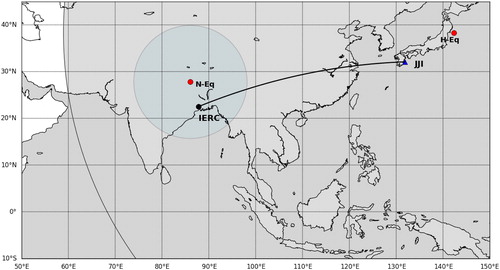
Table 1. Basic earthquake information.

Eq	Location of epicenter	Richter scale magnitude	Depth (km)	Date and time (IST)	Distance (km) from JJI	Distance (km) from IERC	Radius (km) of preparation zone
H-Eq	${38.322}^{°}N,$ ${142.369}^{°}E$	9.0	29	11/03/2011 11:16:24	1180	5438	7413
N-Eq	${27.89}^{°}N,$ ${86.17}^{°}E$	7.3	10	12/05/2015 12:35:19	4392	621	1377

The plate tectonic structure of Japan and surrounding areas is very complex. The Pacific plate, Eurasian plate, North American plate and Philippine plate are the major plates that influence the tectonic structure of Japan. There are also several micro plates that contribute in the plate tectonics of Japan, namely the Okhotsk microplate in northern Japan, the Okinawa microplate in southern Japan, the Yangzee microplate in the area of the East China Sea and the Amur microplate in the area of the Sea of Japan. On 11 March 2011, the Honshu earthquake occurred where the Pacific plate subduct beneath the North American plate at a rate of 83 to 90 millimeter per year. The motion pushes the upper plate and causes a seismic slip-rupture event. The break causes the rise of sea floor by several metres. The seismic moment (M_o) energy, as calculated by the USGS is around 3.9 × 10²² Joules and the surface energy of the seismic waves is around 1.9 × 10¹⁷ Joules. Seismic activity in the Himalayan region is the result from the continental collision of the Indian and Eurasian plates. These two plates are converging at a rate of 40 to 50 millimeter per year. The Indian plate moving northward beneath the Eurasian plate generates numerous number of earthquakes. The surface expression of the plate boundary is marked by the foothills of the north-south trending Sulaiman Range in the west, the Indo-Burmese Arc in the east and the east-west trending Himalaya Front in the north of India. The narrow Himalaya Front has the highest rate of seismic activity and largest earthquakes. The main reason behind the highest rate of seismic activity in this region is the movement on thrust faults. The epicentre of 12 May 2015 Nepal earthquake is also on the same fault. The seismic moment (M_o) energy, is around 1.1 × 10²⁰ Joules and the surface energy of the seismic waves is around 5.6 × 10¹⁵ Joules.

In this study, we have used the VLF data recorded by the SoftPAL (Software Phase and Amplitude Logger) VLF antenna/receiver system. We used electric field antenna coupled with pre-amplifier and service unit. The service unit provides the electrical power to the pre-amplifier and the global positioning system (GPS) unit. The data are being stored by a USB dongle and Lab-chart software with a time stamped by the GPS unit.

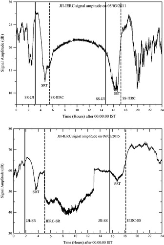
In Figure 2(a,b), we present a typical diurnal variation of JJI-IERC signal amplitude as a function of time in hours as recorded on 5 March 2011, 6 days prior to H-Eq and 9 May 2015, 3 days prior to N-Eq as the receiver is out of order from 22 April 2015 to 7 May 2015 due to technical problems. Our prime focus is the movement of the unperturbed Sunrise Terminator Time (SRT) during the two seismic events. In Figure 2(a,b), the minimum after the actual sunrise is noted as SRT. The second VLF terminator (Sunset Terminator Time or SST) is also indicated in the Figures. The signal shows clear day and night-time usual variation with true sunrise and sunset phenomena.

Figure 2. Diurnal variation of VLF signal amplitude as a function of time (in hours) as received at IERC along the path JJI-IERC for 5 March 2011 (a) and for 9 May 2015 (b). The SRT and SST are the sunrise and sunset terminator time respectively. This signal is treated as seismically quiet as the date is far from the earthquake day and the value of the SRT is treated as unperturbed value.

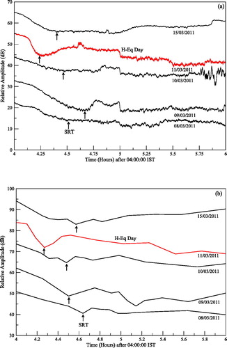
To understand the gradual or sudden movements of the SRTs during and prior to earthquakes, we present the variation of SRT during both the earthquakes in Figures 3 and 4. In Figure 3, the SRT variation for H-Eq is presented from 8 March to 15 March 2011. After the earthquake occurred, the JJI transmitter was turned off during 12 March to 14 March 2011. The signals are stacked with an amplitude shift of 10 dB for a better understanding of the SRT shifts (Figure 3). The red colour plot represents the earthquake day. The value of SRT on May 9 has been taken as the normal or unperturbed value. On the next day, there is a shift of SRT towards daytime and after that small gradual shifts occurred towards night-time from May 10. On May 11, the SRT shift is maximum. After that it again started to come to normal or unperturbed condition on 15th. This can be due to the effects of aftershocks which followed the main shock and continued up to March 16. The effect is most prominent on March 11 which is itself the day of the quake.

Figure 3. Daily variation of sunrise terminator time (SRT) as a function of time in hours from 8 March 2011 to 15 March 2011. Along X-axis time is plotted in hours starting from 03:00:00 IST to 06:00:00 IST and along Y-axis relative amplitude in dB is plotted. The signal amplitudes are stacked with a shift by 10 dB each. The SRTs are indicated by arrows. The earthquake that occurred 11 March 2011 is marked with red colour. The shift of SRT is maximum on the day of the earthquake.

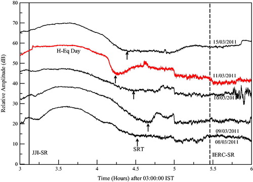
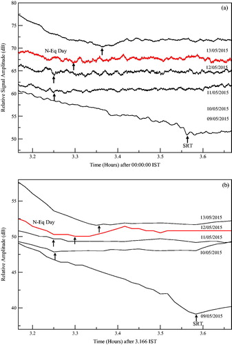
Figure 4. Daily variation of sunrise terminator time (SRT) as a function of time in hours from 9 May 2015 to 13 May 2015. Along X-axis time is plotted in hours starting from 02:00:00 IST to 05:00:00 IST and along Y-axis relative amplitude in dB is plotted. The signal amplitudes are stacked with a shift by 10 dB each. The SRTs are indicated by arrows. The earthquake that occurred on 12 May 2015 is marked with red colour. The shift of SRT is maximum on 1 day before the earthquake.

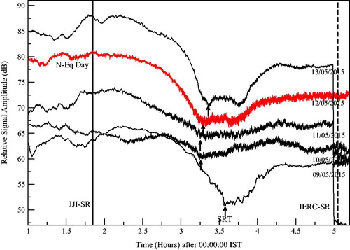
In a similar way, we present the SRT variation for N-Eq in Figure 4 for the duration from 9 May to 13 May 2015. The signals are similarly stacked and the red colour data is for the earthquake day. On the contrary to H-Eq, for N-Eq the SRT shifts are quite gradual and unidirectional towards night-time. The shift started on May 10 and it became maximum on May 11 which is one day before the earthquake. It started returning to the normal position on May 12 but did not reach it which may be due to the similar reasons of aftershocks. For both the cases, the SRT shift is highly prominent. The difference due to seismic perturbation for N-Eq is that the change is more gradual than H-Eq. Also the major effects are pre-seismic for N-Eq whereas for H-Eq it is co-seismic, that is, it happens on the day of the earthquake.

3. Numerical simulation

To reproduce the observed VLF signal variation during both the earthquakes, we coupled our observational data of VLF signal amplitude with the LWPC code (Ferguson 1998). The LWPC code is based on wave-guide mode theory of radio wave propagation. It is a collection of programmes which is used to estimate the VLF signal profile corresponding to the given D-region conditions for which one has to provide the suitable boundary conditions for the lower and upper wave-guide boundaries. The lower boundary parameters related to the wave-guide propagation, that is, the grid based global map of permittivity and conductivity (σ) of the earth are embedded in the code itself. It is chosen according to the characteristics of a baseline. The upper wave-guide boundary, that is, the D-region ionosphere is specified by the two component-exponential Wait’s model having its major components, such as, electron density $N_e(h)$ and the electron-neutral collision frequency (σ_h) (Wait and Spies 1964; Pal and Chakrabarti 2010). In the Wait’s exponential lower ionosphere model, the electron density is related to the steepness parameter (β) and reference height ($h\prime$) as given by the equation, (1) $$N_e(h,h\prime ,\beta )\sim e^{\left(0.15h^{\prime }\right)}{e}^{\left[\right(\beta -0.15\left)\right(h-h^{\prime }\left)\right]}.$$(1)

In this paper, we used RANGE model of LWPM programme (which is incorporated in LWPC) and the subprogram EXPONENTIAL. First, we supplied the transmitter, receiver and propagation path information to RANGE as input. The JJI-IERC propagation path is a typical example of mid-latitude path (${22.5}^{°}$N to ${32}^{°}$N), where it is justified to neglect the latitude variation of D-region ionospheric characteristics. On the other hand, this path is significantly spreaded over longitude (${87}^{°}$E to ${130}^{°}$E). Hence, a notable contrast of solar irradiation induced net D-region ionization and electron content are present over the entire path, especially during sunrise and sunset terminator movements across it. To accommodate all these dynamic path variations of ionosphere using the Wait’s exponential ionospheric model, we replaced it with a dynamic mean D-region ionospheric variation and accordingly it was represented by a set of ‘$h_{\mathit{eff}}^{\prime }$ and β_eff’. We normalized the observed VLF amplitude to the values corresponding to the unperturbed ionospheric condition as defined by LWPC. Second, we ran the RANGE to reproduce the temporal trend of the observed VLF amplitude for a single day by supplying suitable values of these β_eff and $h_{\mathit{eff}}^{\prime }$ values in the EXPONENTIAL. Third, we repeated this simulation procedure to reproduce the temporal trend of the normalized VLF amplitude for a few days around both the earthquake days, especially around the VLF-SRT and estimated the effective parameters. Fourth, we calculated the altitude profile of D-region electron density ($N_e(h)$) from those effective parameters using Wait’s model (see Equation (1)(1) $$N_e(h,h\prime ,\beta )\sim e^{\left(0.15h^{\prime }\right)}{e}^{\left[\right(\beta -0.15\left)\right(h-h^{\prime }\left)\right]}.$$(1) ) particularly at the respective VLF-SRTs of those days. According to LWPC, the $h_{\mathit{eff}}^{\prime }=74$ km and ${\beta }_{\mathit{eff}}=0.3$ km⁻¹ represents the total ionospheric-day condition and $h_{\mathit{eff}}^{\prime }=87$ km and ${\beta }_{\mathit{eff}}=0.6k{m}^{-1}$ represents a complete night. During this simulation, the β_eff and $h_{\mathit{eff}}^{\prime }$ varied within 0.4 to 0.55 km⁻¹ and 78 to 82.5 km for N-Eq. For the case of H-Eq, the same varied within 0.35 to 0.6 km⁻¹ and 76 to 80 km. Practically, β_eff and $h_{\mathit{eff}}^{\prime }$ values in these ranges effectively represent the mixed day-night conditions over the path.

4. Results and interpretation

We present the observed and simulated temporal variation of VLF-SRTs during both the earthquakes. In Figure 5(a,b), we present the observational VLF signal amplitude as a function of time starting from 04:00:00 to 06:00:00 IST and the corresponding simulated amplitude (lower panel) for the same time period for H-Eq. In both the figures, the black curves and the red curve indicate the signal on the normal days and the earthquake day, respectively. The VLF signal amplitudes are stacked in a similar manner as presented in Section 2. The arrows indicate corresponding VLF-SRTs. From Figure 5(a,b), we can clearly see that the SRTs are shifted towards night-time and reaches the maxima on 11 March 2011, that is, the H-Eq day which satisfies our observation. The net shift of VLF-SRT observed on March 11 compared to March 8 (normal day) is ∼18.4 minutes, whereas the same obtained from simulation is ∼20.2 minutes.

Figure 5. Comparison of observed (upper panel) and simulated (lower panel) amplitude variation around the SRTs during the H-Eq. Both the observed and simulated signal amplitudes are plotted as a function of time in hours for an interval of 04:00:00 to 06:00:00 IST. The black curves and the red curve denote the seismic quiet and active days respectively. The VLF-SRTs are marked with arrows. The simulated signal and especially the shift of the SRTs matches quite satisfactorily with the observed values. The shift in VLF-SRTs is maximum on the day of the H-Eq.

Figures 6(a,b) present the similar works, but for N-Eq. Here, we present the observational VLF signal amplitude for the duration from 03:09:57 to 03:40:60 IST. We choose the time span in such a way that the position of the VLF-SRT is in the middle and the temporal variation is clearly understandable. We also present the simulated counterpart of it for the same time period in Figure 6(b). We can clearly see that the shift of VLF-SRT towards night-time is more gradual than H-Eq. Here, it reaches the maxima on 11 May 2015, that is, a day before the N-Eq which is also evident from our observation. The net shift of VLF-SRT observed on May 11 compared to May 9 is ∼19.1 minutes, whereas the same computed from simulation is ∼20.4 minutes. The net observed VLF-SRT shift on the earthquake day, that is, May 12 as compared to May 9 is 16.2 minutes, whereas the same obtained from simulation is 16.6 minutes. It can be clearly seen that the shift is decreased by (19.1–16.2)= 2.9 minutes which indicates that the D-region ionospheric recovery processes have already been initiated and the VLF-SRT started returning to its original value right from the earthquake day. This phenomenon is in contrary to the H-Eq case, where the same recovery mechanism started 2–3 days after the day of the earthquake (Figure 5(a,b)). The possible reason behind this contradiction may be associated with the location of the two epicentres in reference to the receiving location, IERC.

Figure 6. Comparison of observed (upper panel) and simulated (lower panel) amplitude variation around the SRTs during the N-Eq. Both the observed and simulated signal amplitudes are plotted as a function of time in hours for an interval of 03:09:57 to 03:40:60 IST. The black curves and the red curve denote the seismic quiet and active day respectively. The VLF-SRTs are marked with arrows. The simulated signal and especially the shift of the SRTs matches quite satisfactorily with the observed values. The shift in VLF-SRTs is maximum on one day prior to the N-Eq.

In Figures 7 and 8, we present the altitude profile of electron densities ($N_e(h)$) in $m^{-3}$ in logarithmic scale obtained from Wait’s ionospheric model at VLF-SRTs on the days of and around H-Eq and N-Eq respectively. In Figure 7, the $N_e(h)$s are calculated at VLF-SRT of 8 March 2011, which is treated as a quiet day for H-Eq. For altitudes above 78 km, the $N_e(h)$ decreases as one approaches the day of H-Eq. The $N_e(h)$ change is sudden from March 9 to March 10 by an amount of ∼40% at a height of 82 km and interestingly the corresponding VLF-SRT change is also comparatively higher (∼20.4 minutes). The $N_e(h)$ does not change much from 11 March 2011 to 15 March 2011 possibly due to a series of aftershocks that took place at that time and it did not allow the ionosphere to return to the so called quiet or unperturbed state.

Figure 7. The height profile of electron density (logarithmic scale) in $m^{-3}$ for a duration of 8 March to 11 March and 15 March 2011 as calculated from effective ionospheric parameters and Wait’s exponential formula. To understand the variation more clearly, the graphs are redrawn in the inset. The values are calculated for the time of SRT of March 8 which is treated as normal day. For altitude above 78 km, the electron density decreases as one approaches to the earthquake day. The change is sudden from March 10 to March 11 and the value of N remains in almost same level after March 11 due to a series of aftershocks that followed the main shock.

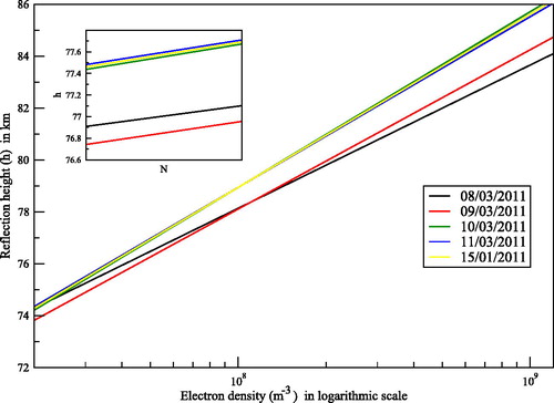
Figure 8. The height profile of electron density (logarithmic scale) in $m^{-3}$ for a duration of 9 May to 13 May 2015 as calculated from effective ionospheric parameters and Wait’s exponential formula. The values are calculated for the time of SRT of May 9 which is treated as normal day. For a particular height, the electron density decreases gradually as one approaches to the earthquake day. It became minimum on May 11. After that it stated increasing and on May 13 reaches almost the same level from where it started initially. The change is quite gradual rather than the H-Eq.

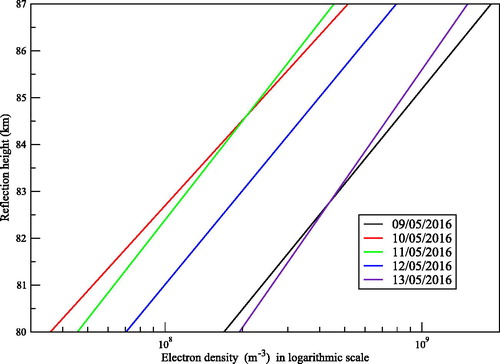
In Figure 8, the electron density profile $N_e(h)$ as a function of reflection height is presented at the time of VLF-SRT of 9 May 2015, which is treated as normal day for N-Eq. In a similar manner, for altitudes above 80 km, the electron density decreases gradually as one approaches the earthquake day. The value of $N_e(h)$ became minimum on May 11. After that it started increasing and on May 13, it reached almost the same level from where it started initially. The maximum change of $N_e(h)$ from May 9 to May 11 is around 76%.

To highlight the solar geo-magnetic effects in our results, we checked the solar geo-magnetic k_p index during our observation. For H-Eq, the k_p values were moderate (${\mathrm{k}}_{p}5$). For N-Eq, it was found geo-magnetically quiet for almost the entire duration of our study (${\mathrm{k}}_{p}3$) except on May 13 when it was moderate with ${\mathrm{k}}_{p}5.$

5. Discussion

In this paper, our prime focus was to study the VLF signal anomalies related to possible ionospheric perturbations due to two earthquakes whose epicentres were far away and situated on the same VLF propagation path in such a way that one was closer to the transmitter and the other to the receiver. The two earthquakes chosen were the Honshu earthquake that occurred on 11 March 2011 and the Nepal earthquake that occurred on 12 May 2015. These two earthquakes were in the vicinity of the transmitter JJI and the receiver IERC respectively. We observed significant shift in VLF-SRTs towards night-time for both the quakes. We numerically reproduced the temporal profile of signal amplitude which includes the shifts in SRT by using LWPC model. We computed the normal and seismically perturbed electron density profiles during these events using Wait’s formula. We found significant differences in the behaviour of VLF signals for these two earthquakes. For H-Eq, which was closer to the transmitter, the study showed sudden change in the SRT shift and the effect is co-seismic in nature, that is, the maximum shift occurred on the day of the earthquake. On the other hand, for N-Eq, the shifts are quite gradual and pre-seismic, that is, the maximum effects in the signal is one day prior to the earthquake. This is also reflected in the simulation and we found the expected sudden and gradual trend in the $N_e(h)$ profile for H-Eq and N-Eq, respectively. There are notable quantitative differences present in the change of $N_e(h)$ profile at 82 km and the change is larger for the N-Eq (76%) than H-Eq (40%). For the two earthquakes, the JJI signal propagated through two distinct conditions. For, H-Eq, it travelled from a higher seismically perturbed region to a lower one but for N-Eq just the opposite situation happened where it went from an unperturbed zone to a highly perturbed one. These differences in signal anomalies can be connected with these relative locations of the epicentres of the two earthquakes and the characteristics of the propagation path.

6. Conclusion

The LAIC mechanism relates properties of apparently distant and distinct components of Earth system science ranging from lithosphere, lower ionospheric D-layer to upper F2 layer. Starting from the tropospheric thermal anomalies, lower ionospheric electron density variation to upper ionospheric critical frequency modulation, LAIC takes into account a wide range of geo-chemical and geo-physical phenomena which could be affected simultaneously. As yet, there is no concrete idea of how and why exactly the lithospheric variabilities percolate into ionospheric irregularities. However, our study proves that such changes do occur. Study of physical mechanisms behind the LAIC, implementing acquired knowledge for future earthquake prediction and regular monitoring of such parameters is absolutely essential to achieve our goal. Study of VLF wave propagation for multiple paths and also for various earthquakes at the same time can reveal more easy way of understanding the exact cause-effect scenario of seismo-ionospheric coupling.

Acknowledgements

SG, SS, TB and SKC acknowledge Govt. of West Bengal, India for supporting the research. SC acknowledges the Post-doctoral fellowship of the S. N. Bose National Centre for Basic Sciences for providing financial support towards completion of this research.

Disclosure statement

No potential conflict of interest was reported by the authors.

References

- Baba K, Hayakawa M. 1996. Computational results of the effect of localized ionospheric perturbations on subionospheric VLF propagation. J Geophys Res. 101(A5):10985–10993.
- Chakrabarti S, Sasmal S, Saha M, Khan M, Bhowmik D, Chakrabarti SK. 2007. Unusual behavior of D-region ionization time at 18.2 kHz during seismically active days. Indian J. Phys. 81:531–538.
- Chakrabarti SK, Saha M, Khan R, Mandal S, Acharyya K, Saha R. 2005. Possible detection of ionospheric disturbances during Sumatra-Andaman Islands earthquakes in December. Indian J Radio Space Phys. 34:314–317.
- Chakrabarti SK, Sasmal S, Chakrabarti S. 2010. Ionospheric anomaly due to seismic activities-Part 2: evidence from D-layer preparation and disappearance times. Nat Hazards Earth Syst Sci. 10(8):1751–1757.
- Chakrabarti SK, Sasmal S, Ray S. 2012. Short term earthquake prediction using VLF observations: an ICSP initiative. In: Hayakawa M, editor. Indian sub-continent, frontier of earthquake prediction. Nihon-senmon-Tosho Pub. Comp, Tokyo.
- Chakraborty S, Sasmal S, Basak T, Ghosh S, Palit S, Chakrabarti SK, Ray S. 2017. Numerical modeling of possible lower ionospheric anomalies associated with Nepal earthquake in May, 2015. Adv Space Res. 60(8):1787–1796.
- Clilverd MA, Rodger CJ, Thomson NR. 1999. Investigating seismo-ionospheric effects on a long subionospheric path. J Geophys Res. 104(A12):28171–28179.
- Dobrovolsky IP, Zubkov SI, Miachkin VI. 1979. Estimation of the size of earthquake preparation zones. PAGEOPH. 117(5):1025–1044.
- Ferguson JA. 1998. Computer programs for assessment of long wavelength radio communications, Version 2.0. Technical document 3030. San Diego (CA): Space and Naval Warfare Systems Center.
- Gokhberg MB, Gufeld IL, Rozhnoy AA, Marenko VF, Yampolsky VS, Ponomarev EA. 1989. Study of seismic influence on the ionosphere by super long-wave probing of the Earth ionosphere wave-guide. Phys Earth Planet Inter. 57(1-2):64–67.
- Gokhberg MB, Nekrasov AK, Shalimov SL. 1996. On the influence of unstable release of green-effect gases in seismically active regions on the ionosphere. Izv Earth Phys. 8:52–57.
- Hayakawa M. 1999. Atmospheric and ionospheric electromagnetic phenomena associated with earthquakes. Tokyo: Terra Sci. Pub. Co.; 996 p.
- Hayakawa M, Fujinawa Y. 1994. Electromagnetic phenomena related to earthquake prediction. Tokyo: Terra Sci.
- Hayakawa M, Kasahara Y, Nakamura T, Muto F, Horie T, Maekawa S, Hobara Y, Rozhnoi A, Solovieva M, Molchanov OA. 2010. A statistical study on the correlation between lower ionospheric perturbations as seen by subionospheric VLF/LF propagation and earthquakes. J Geophys Res. 115:A09305.
- Hayakawa M, Molchanov OA. 2002. Seismo electromagnetics: lithosphere - atmosphere - ionosphere coupling. Tokyo: TERRAPUB, 477 p.
- Hayakawa M, Molchanov OA, Ondoh T, Kawai E. 1996a. Anomalies in the sub-ionospheric VLF signals for the 1995 Hyogo-ken Nanbu earthquake. J Phys Earth. 44(4):413–418.
- Hayakawa M, Molchanov OA, Ondoh T, Kawai E. 1996b. The precursory signature effect of the Kobe earthquake on VLF subionospheric signals. J Commun Res Lab, Tokyo. 43:169–180.
- Hayakawa M, Ohta K, Nickolaenko AP, Ando Y. 2005. Anomalous effect in Schumann resonance phenomena observed in Japan, possibly associated with the Chi-chi earthquake in Taiwan. Ann Geophys. 23(4):1335–1346.
- Hayakawa M, Sato H. 1994. Ionospheric perturbations associated with earthquakes as detected by subionospheric VLF propagation. In: Hayakawa M, Fujinawa Y, editors. Electromagnetic phenomena related to earthquake prediction. Tokyo: Terra Sci.; p. 391–397.
- Hegai V, Kim VP, Liu JY. 2006. The ionospheric effect of atmospheric gravity waves excited prior to strong earthquake. Adv Space Res. 37(4):653–659.
- Hickey MP, Schubert G, Walterscheild RL. 2009. Propagation of tsunami driven gravity waves into the thermosphere and ionosphere. J Geophys Res. 114:A08304.
- Horie T, Maekawa S, Yamauchi T, Hayakawa M. 2007a. A possible effect of ionospheric perturbations associated with the Sumatra earthquake, as revealed from subionospheric very-low-frequency (VLF) propagation (NWC-Japan). Int J Remote Sens. 28(13-14):3133–3139.
- Horie T, Yamauchi T, Yoshida M, Hayakawa M. 2007b. The wave like structures of ionospheric perturbation associated with Sumatra earthquake of 26 December 2004, as revealed from VLF observation in Japan of NWC signals. J Atmos Sol-Terr Phys. 69(9):1021–1028.
- Korepanov V, Hayakawa M, Yampolski Y, Lizunov G. 2009. AGW as a seismo-ionospheric coupling responsible agent. Phys Chem Earth. 34(6-7):485–495.
- Lin’kov EM, Petrova LN, Osipov KS. 1990. Seismogravity pulsations of the Earth and atmospheric disturbances as possible precursors of strong earthquakes. Doklady RAN. 313:239–258.
- Liperovsky VA, Mikhailin VV, Shevtsov BM, Umarkhodgajev PM, Bogdanov VV, Meister C-V. 2007. Electrical phenomena in aerosol clouds above faults regions before earthquakes. In Shevtsov BM, editor. Proc. 4th Int. Conf. Solar-Earth connections and earthquake precursors in Paratunka (Kamchatka region); 14–17 August 2007. IKIR FEB RAS. p 391–398.
- Longnonne P. 2010. Seismic waves from atmospheric sources and atmospheric/Ionospheric signatures of seismic waves. In: Infrasound monitoring for atmospheric studies. Dordrecht (The Netherlands): Springer; p. 281–304.
- Mikhailov YM, Mikhailovna GA, Kapustina OV, Buzevich AV, Smirnov SE. 2004. Power spectrum features of near-earth atmospheric electric field in Kamchatka. Ann Geophys. 47:237–245.
- Mikhailov YM, Mikhailovna GA, Kapustina OV, Buzevich AV, Smirnov SE. 2005. Special features of atmospheric noise superimposed on variations in the quasistatic electric field in the Kamchatka near-earth atmosphere. Geomag Aeron. 45:649–665.
- Molchanov OA. 2009. Lithosphere-atmosphere-ionosphere coupling due to seismicity. In: Hayakawa, M., editor, Electromagnetic phenomena associated with earthquakes; p. 255–279, Transworld Research Network, Trivandrum.
- Molchanov OA, Hayakawa M. 1998. Subionospheric VLF signal perturbations possibly related to earthquakes. J Geophys Res. 103(A8):17489–17504.
- Molchanov OA, Hayakawa M, Oudoh T, Kawai E. 1998. Precursory effects in the subionospheric VLF signals for the Kobe earthquake. Phys Earth Planet Inter. 105(3-4):239–248.
- Nemec F, Santolik O, Parrot M. 2009. Decrease of intensity of ELF/VLF waves observed in the upper ionosphere close to earthquakes: a statistical study. J Geophys Res. 114(A4): A04303.
- Pal S, Chakrabarti SK. 2010. Theoretical models for Computing VLF wave amplitude and phase and their applications. AIP Conf Proc. 1286:42–60.
- Pal P, Sasmal S, Chakrabarti SK. 2017. Studies of seismo-ionospheric correlations using anomalies in phase of very low frequency signal. Geomat Nat Hazards Risk. 8(2):167–176.
- Pulinets SA. 1998. Seismic activity as a source of the ionospheric variability. Adv Space Res. 22(6):903–906.
- Pulinets S, Boyarchuk K. 2004. Ionospheric precursors of earthquakes. Berlin: Springer.
- Pulinets SA, Boyarchuk KA, Hegai VV, Kim VP, Lomonosov AM. 2000. Quasielectrostatic model of atmosphere-thermosphere-ionosphere coupling. Adv Space Res. 26(8):1209–1218.
- Pulinets S, Liu JY. 2004. Ionospheric variability unrelated to solar and geomagnetic activity. Adv Space Res. 34(9):1926–1933.
- Pulinets S, Ouzounov D. 2011. Lithosphere-atmosphere-ionosphere coupling (LAIC) model–an unified concept for earthquake precursors validation. J Asian Earth Sci. 41(4-5):371–381.
- Pulinets SA, Ouzounov D, Karelin AV, Boyarchuk KA, Pokhmelnykh LA. 2006. The physical nature of thermal anomalies observed before strong earthquakes. Phys Chem Earth. 31(4-9):143–153.
- Ray S, Chakrabarti SK. 2013. A study on the behavior of the terminator shifts using multiple VLF propagation paths during Pakistan earthquakes (M = 7.4), occurred on 19th Jan., 2011. Nat Hazards Earth Syst Sci. 13(6):1501–1506.
- Ray S, Chakrabarti SK, Mondal SK, Sasmal S. 2011. Ionospheric anomaly due to seismic activities-III: correlation between night time VLF amplitude uctuations and effective magnitudes of earthquakes in Indian sub-continent. Nat Hazards Earth Syst. Sci. 11(10):2699–2704.
- Ray S, Chakrabarti SK, Sasmal S. 2012. Precursory effects in the nighttime VLF signal amplitude for the 18th January, 2011 Pakistan earthquake. Indian J Phys. 86(2):85–88.
- Ray S, Chakrabarti SK, Sasmal S, Choudhury AK. 2010. Correlations between the anomalous behavior of the ionosphere and the seismic events for VTX-MALDA VLF Propagation. AIP Conf Proc. 1286:298–308.
- Rodger CJ, Thomson NR, Dowden RL. 1996. A search for ELF/VLF activity associated with earthquakes using ISIS satellite data. J Geophys Res. 101(A6):13, 369–13, 378.
- Rodger CJ, Thomson NR, Wait JR. 1999. VLF scattering from red sprites: vertical columns of ionization in the Earth-ionosphere waveguide. Radio Sci. 34(4):913–921.
- Rozhnoi A, Molchanov O, Solovieva M, Gladyshev V, Akentieva O, Berthelier JJ, Parrot M, Lefeuvre F, Biagi PF, Castellana L, Hayakawa M. 2007. Possible seismo-ionosphere perturbations revealed by VLF signals collected on ground and on a satellite. Nat Hazards Earth Syst Sci. 7(5):617–624.
- Sasmal S, Chakrabarti SK. 2009. Ionospheric anomaly due to seismic activities - I: calibration of the VLF signal of VTX 18.2 kHz station from Kolkata. Nat Hazards Earth Syst Sci. 9(4):1403–1408.
- Sasmal S, Chakrabarti SK. 2010. Studies of the correlation between ionospheric anomalies and seismic activities in the Indian subcontinent. AIP Conf Proc. 1286:270–290.
- Sasmal S, Chakrabarti SK, Ray S. 2014. Unusual behavior of VLF signals observed from Sitapur during the Earthquake at Honshu, Japan on 11 March, 2011. Indian J Phys. 88(10):1013–1019.
- Shvets AV, Hayakawa M, Molchanov OA, Ando Y. 2004. A study of ionospheric response to regional seismic activity by VLF radio sounding. Phys Chem Earth. 29(4-9):627–637.
- Sorokin VM, Chmyrev VM. 2002. Electrodynamic model of ionospheric precursors of earthquakes and certain types of disasters. Geomagn Aeron. 42(6):784.
- Sorokin VM, Yashchenko AK. 1999. Conductivity and electric field disturbance in the earth-ionospheric layer above the impending earthquake source. Geomagn Aeron. 39(2):100.
- Wait JR. 1962. Electromagnetic waves in stratified media. New York (NY): Pergamon Press.
- Wait JR, Spies KP. 1964. Characteristics of the earth-ionosphere waveguide for VLF radio waves, NBS Tech. Note 300. Gaithersburg (MD): Nat. Inst. Stand. Technol.