Novel hybrids of adaptive neuro-fuzzy inference system (ANFIS) with several metaheuristic algorithms for spatial susceptibility assessment of seismic-induced landslide

Abstract

Strong ground motions usually trigger lots of slope failures in the affected area. In this work, we analyse the occurrence likelihood of earthquake-triggered landslide by employing the ensembles of adaptive neuro-fuzzy inference systems (ANFIS) with four well-known metaheuristics techniques, namely particle swarm optimization (PSO), genetic algorithm (GA), ant colony optimization (ACO), and differential evolution (DE) algorithms. Twelve landslide conditioning factors namely, elevation, slope degree, lithology, peak ground acceleration (PGA), stream power index (SPI), topographic wetness index (TWI), distance to road, distance to river, distance to fault, normalized difference vegetation index (NDVI), slope aspect, and plan curvature are considered within the geographic information system (GIS) to produce the required spatial database. In this paper, frequency ratio (FR) model is used to evaluate the spatial interaction between the landslides and conditioning factors. Meantime, among a total of 458 marked earthquake-induced landslides, 366 (80%) are specified to the learning process, and the remaining 92 (20%) landslides are used to evaluate the accuracy of applied models. The landslide susceptibility maps are generated in the GIS environment. Three accuracy criteria of mean square error (MSE), root mean square error (RMSE), and area under the receiving operating characteristic curve (AUROC) are used to develop a ranking system for comparing the integrity of the designed models. The total ranking scores (TRSs) of 15, 8, 10, and 18, respectively, obtained for PSO-ANFIS, GA-ANFIS, ACO-ANFIS, and DE-ANFIS revealed the superiority of the DE algorithm compared to other metaheuristics techniques. Also, the DE-ANFIS emerged as the fastest ensemble, due to the highest convergence speed obtained for this model.

Keywords:

• Earthquake-triggered landslide
• geographic information system
• ANFIS
• evolutionary optimization
• landslide susceptibility mapping

1. Introduction

As a widespread disaster, landslides cause severe loss of property and human life worldwide. China has been faced with numerous landslides, mostly due to the strong ground motions which bring huge slope failures. Ludian earthquake, for example, occurred at 4.30pm on 3 August 2014, at a focal depth of 12 km (Hong et al. 2016b). The intensity was reported as M6.5 with an epicentre located at 27°14′42″ N and 103°25′37″ E. The meizoseismal area’s peak ground acceleration (PGA) reached 948.5 cm/s², according to the U.S Geological Survey (USGS). Also, the depth of the aftershocks ranged between 3 km and 15 km (Cheng et al. 2015). This earthquake killed 617 people and caused 3143 injuries. Moreover, thousands of houses ruined or seriously damaged by the Ludian earthquake. Even though various methods have been proposed to investigate the seismic landslide, it has remained a serious problem for scientists. Up to now, different landslide assessment methods have been developed to appraise the risk of landslide occurrence in a particular study area (Moayedi et al. 2011; Pham et al. 2018; Yan et al. 2018; Nguyen et al. 2019; Xi et al. 2019; Yang et al. 2019; Yuan and Moayedi 2019; Moayedi et al. 2019b). Xie et al. (2015) provided the landslide susceptibility map of the Ludian after the Ludian 2014 earthquake by using random forest model. With approximate accuracy of 92%, they concluded that 80% of the marked landslides are in the areas that have been categorized as moderate and high landslide risk.

Lots of researchers have investigated the possibility of landslide occurrence by providing landslide susceptibility maps or generating formulas to calculate the landslide hazard index (Pradhan 2010; Pourghasemi et al. 2013; Regmi et al. 2014; Youssef et al. 2015; Vakhshoori and Zare 2016; Hong et al. 2016a). These studies have mainly considered the altitude, aspect, soil type, slope, vegetation density, lithology, distance from linear phenomena like faults, rivers and roads, stream power index (SPI), etc. as the landslide conditioning factors. Moreover, plenty of studies have outlined the landslide risk evaluation by means of simple predictive methods like statistical index (SI), frequency ratio (FR), weights of evidence (WoE) or regression-based approaches (Demir et al. 2015; Youssef et al. 2015; Chen et al. 2016). Chen et al. (2018a) proposed three ensembles of evidential belief function (EBF), SI, and WoE approaches with kernel logistic regression (KLR) for landslide hazard zonation at Chongren of China. Referring to the calculated area under the curve (AUC) as well as the prediction rate (AUC_P) and success rate (AUC_T) criteria, it was demonstrated that EBF-KLR (with AUC = 0.753, AUC_P = 0.7615, and AUC_T = 0.8511) presents the most reliable prediction, followed by SI-KLR and WoE-KLR hybrid methods.

Also, looking for more reliable approximations, soft artificial intelligence methods have been used and emerged as effective approaches for landslide risk analyse (Yao et al. 2008; Zare et al. 2013; Pham et al. 2018; Shirzadi et al. 2018; Binh Thai et al. 2018a; Dieu Tien et al. 2018a; Chen et al. 2018b; Polykretis et al. 2019; Tian et al. 2019; Chen et al. 2019d). In a research carried out by Lee et al. (2017), support vector machine (SVM) was successfully used to map the landslide hazard in PyeongChang and Inje districts of Gangwon Province, Korea. Referring to the obtained accuracies 81.36% and 77.49%, they found that the SVM can be effectively used for this aim. Also, numerous comparative attempts have dealt with evaluating the applicability of different developed models. Chen et al. (2017) examined the integrity of three state-of-the-art intelligent models namely, adaptive neuro-fuzzy inference system combined with frequency ratio (ANFIS-FR), generalized additive model (GAM), and SVM in landslide hazard mapping in Hanyuan County, China. This study showed that SVM outperforms ANFIS-FR and GAM with respective accuracies of 87.5%, 85.1%, and 84.6%. Bui et al. (2016) applied five predictive tools including SVMs, multi-layer perceptron neural networks (MLP Neural Nets), radial basis function neural networks (RBF Neural Nets), KLR, and logistic model trees (LMT) to model the risk of landslide in Son La hydropower basin, Vietnam. To select the most compatible subset of conditioning factors, they used a k-fold cross-validation technique. The results of this paper revealed that MLP and SVR could perform more efficiently than RBF, KLR, and LMT.

Likewise, robust evolutionary techniques have been effectively applied to improve the applicability of typical intelligent models (Bui et al. 2017b; Moayedi et al. 2019b; Gao et al. 2018a; Binh Thai et al. 2018b; Dieu Tien et al. 2018b; Gao et al. 2018b; Tien Bui et al. 2018b; Binh Thai et al. 2018c; Gao et al. 2018c, 2018d, 2019; Jaafari et al. 2019; Chen et al. 2019b). In this sense, Moayedi et al. (2019b), compared the efficiency of multilayer perceptron neural network against its improved version, that is, artificial neural network synthesized with particle swarm optimization algorithm (PSO-ANN), in landslide susceptibility modelling at Kermanshah province, west of Iran. They considered 12 landslide conditioning factors including elevation, plan curvature, lithology slope aspect, slope degree, soil type, distance to road, distance to river, distance to fault, SPI, topographic wetness index (TWI), as the landslide-independent parameters. As the main result of this study, they found particle swarm optimization (PSO) performs as a promising optimization algorithm for landslide hazard assessment. Li et al. (2017) employed a new genetic algorithm (GA) for optimal selection of landslide-related factors in Wenchuan, Ludshan, and Ludian areas, China. Considering the acquired AUCs of 93.48% and 93.47%, 83.48% and 83.45%, and 82.28% and 82.21%, respectively in Wenchuan, Lushan, and Ludian districts, the proposed method outperformed the typical GA. Moreover, differential evolution (DE) algorithm was satisfactorily used by Bui et al. (2016) to find the optimal tuning parameters of least-squares support vector machines (LSSVM) model in hazard assessment of rainfall-induced shallow landslide in central Vietnam. Their results revealed the superiority of the proposed models (with the approximate accuracy of 82%) in comparison with SVMs, multi-layer perceptron neural networks (MLP), and J48 decision trees. The applicability of three optimization methods namely, GA, DE, and PSO synthesized with the adaptive neuro-fuzzy inference system (ANFIS) for landslide spatial modelling was evaluated by Chen et al. (2017). Referring to the acquired AUC values, they introduced the ANFIS-DE (AUC = 0.844) as the most accurate ensemble data mining technique, compared to ANFIS-GA (AUC = 0.821), and ANFIS-PSO (AUC = 0.780).

Besides, similar optimization methods have been successfully used to generate the flood susceptibility map (Ahmadlou et al. 2018; Hong et al. 2018; Termeh et al. 2018; Tien Bui et al. 2018a) or the groundwater spring potential for different areas (Tien Bui et al. 2018a; Chen et al. 2019a, 2019c) through discerning the spatial relationship between the proposed phenomena and related factors. This paper investigates the efficiency of PSO, GA, ant colony optimization (ACO), and DE applied to ANFIS for spatial prediction of the earthquake-induced landslide in Ludian County, China. To this end, after providing the required dataset in the geographic information system (GIS), the proposed models were implemented, and the landslide susceptibility maps were developed. To evaluate the reliability of the results, we used the area under the receiving operating characteristic (ROC) curve (AUROC), mean square error (MSE), and root mean square error (RMSE) of the results.

2. Study area

The study area is located in Ludian district, Yunnan province which is one of the southernmost provinces of China (Figure 1). The area of the selected region is roughly 14877 km² and lies within the east longitude 103°09′ to 103°40′ and north latitude 26°59′ to 27°32′. Topographically, the altitude ranges from 568 to 3356 m, under the monsoon climate. In addition, Dongchuan and Jialing Jian group, Dolomite, Quartzose, sandstone, and Chert Limestone are common rocks in this region. The slope varies in the approximate range of 0–90° so that more than half of this area has the slope lower than 15°. Meanwhile, the average annual values of temperature and rainfall are approximately 12.1 °C and 924 mm. As Figure 1 illustrates, most of the landslides have occurred along the territorial roads and rivers as well as the recognized faults.

Figure 1. Location of the study area and spatial distribution of landslides.

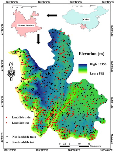
According to Zhou et al. (2016b), which investigated different aspects of the landslides triggered by the Ludian earthquake, this catastrophe occurred at the Baogunao-Xiaohe fault which is located in the Anninghe-Zemuhe-Xiaojiang fault zone. In their study, two useful statistical indices of landslide area ratio (LAR) and landslide density (LD) were calculated for a part of the study area. In this sense, LAR and LD were obtained 2.62% and 2.48 landslides/km². Also, the area of the discovered landslides varies from 76 m² to 0.45 km². About the type of the marked landslides, they are mainly classified as rock falls and shallow, disrupted landslides from steep slopes. Around 20% of the mapped landslides have an area greater than 10,000 m², where 21% of them cover an area greater than 50,000 m². Moreover, around 6% of the landslides cover less than 1000 m² in area. More information are available in Zhou et al. (2016b) and Zhou et al. (2016a).

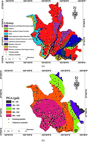
Due to the importance of the seismology and structure geology of the affected area in evaluation of the earthquake effect (Rezaie and Panahi 2015), these maps are presented in Figures 2 and 3(a), respectively. The PGA map of the Ludian earthquake is also shown in Figure 3(b).

Figure 2. The seismology map of the study area (USGS).

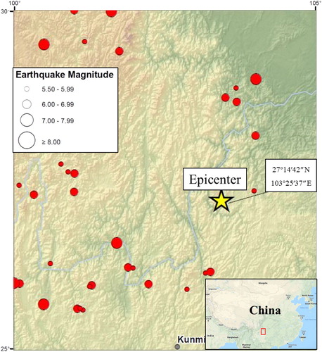
Figure 3. (a) The lithology of the study area and (b) the PGA map of the Ludian earthquake.

3. Data preparation and spatial interaction between the landslide and related factors

Providing the landslide inventory map is a crucial step in any kind of landslide hazard assessment (Ercanoglu and Gokceoglu 2004). In this work, a total of 458 landslide points were identified within the Ludian County utilizing the previous recorded, aerial photos interpretation, and field monitoring using GPS in 1:25,000 scale (see Figure 1). Then, Similar to other studies (Wu et al. 2014; Regmi et al. 2016; Xie et al. 2017; Moayedi et al. 2019b), the landslide locations were randomly divided into two categories containing 366 landslides (80% of whole landslide locations) for training the proposed ensembles and 92 landslides (20% of whole landslide locations) for validating their performance. Remarkably, these points were assigned a value of ‘1’. Next, the same number of non-landslide points was randomly produced over the areas devoid of landslide. They were then divided into the training and testing samples as well, and were assigned a value of ‘0’ (Xie et al. 2017; Chen et al. 2019b).

Considering the landslide-causative parameters of the intended district and also regarding the occurred earthquake, twelve of geological and hydrological landslide-related factors namely, elevation, slope degree, lithology, PGA, SPI, TWI, distance to road, distance to river, distance to fault, normalized difference vegetation index (NDVI), slope aspect, and plan curvature were considered within the GIS. After the preparation process, the mentioned GIS rasters were generated from their initial formats (i.e. polygons, polylines, points, and tabular data).

Similar to Dou et al. (2019), most of the considered conditioning layers were first classified using ‘Natural Breaks’. Table 1 details the spatial distribution of the landslides based on the sub-classes of each effective factor. In the last column of Table 1, the FR of each sub-class is featured indicating the proportion of the observed slope failures over the percentage of domain occupied by the proposed sub-class. Note that, a high correlation is represented by FR value more than 1 and vice versa (Oh et al. 2011). The slope degree, slope aspect and plan curvature GIS layers were derived from the digital elevation model (DEM) of the Ludian County acquired from Landsat 8 imagery. As stated before, elevation varies from 568 to 3356 m so that approximately 82% of the studied area has an altitude between 1300 and 2300. As Table 1 reports, the largest FR for the elevation sub-classes is 2.18 which is obtained for the altitude 1312–1755 m. Slope degree ranges from 0 to 87 degrees. In this factor, the highest and lowest values of FR were 1.32 and 0.87, respectively for the slope groups of [62–87] and [13–33]. From this, it can be concluded that the slope degree is positively correlated with the number of slope failures. Based on the lithology map of Ludian (after Li et al. (2017)), various types of bedrocks suchlike Dongchuan and Jialing Jian group, Dolomite, Quartzose, sandstone, and Chert Limestone form the geology of this area. Accordingly, 46.52% and 13.69% of the slope failures have been observed on the bedrocks labelled as ‘Shale and sandstone (Upper Permian)’ and ‘Shale’, respectively. The seismic parameter of PGA was used to consider the effect of the Ludian earthquake. Note that, PGA is the most commonly used criterion to determine the shaking intensity of damaged area (Nath 2004). For this study, earthquake records were used to draw the PGA map in the GIS environment. Not surprisingly, the more PGA values, the higher the calculated FR. In other words, as we get close to the epicentre, the FR raises which reaches 1.37 for the range of 500–1100 gal. Also, to examine the effect of the geo-morphometric conditions, we calculated two widely-used secondary factors of SPI and TWI. The SPI and TWI parameters respectively symbolize the erosion power of streams and the amount of accumulated water in a place, which are expressed by Equations 1(1) $$\mathit{SPI}= \alpha \times \hspace{0.17em}\text{tan}\hspace{0.17em}\beta$$(1) and 2(2) $$\mathit{TWI}=\mathit{ln}\left(\alpha /\hspace{0.17em}\text{tan}\hspace{0.17em}\beta \right)$$(2) (BEVEN and Kirkby 1979; Moore et al. 1991): (1) $$\mathit{SPI}= \alpha \times \hspace{0.17em}\text{tan}\hspace{0.17em}\beta$$(1) (2) $$\mathit{TWI}=\mathit{ln}\left(\alpha /\hspace{0.17em}\text{tan}\hspace{0.17em}\beta \right)$$(2) where α stands for specific catchment, and β denotes the gradient.

Table 1. Spatial interaction between the landslide and its causative factors.

Factor	Classes	No. of pixels	Percentage of domain	No. of prone pixels	Percentage of prone pixels	FR
Slope degree	0 to 13	3668185	55.03	473991	53.23	0.97
	13 to 33	1038208	15.58	120943	13.58	0.87
	33 to 48	879139	13.19	117403	13.18	1.00
	48 to 62	674754	10.12	106925	12.01	1.19
	62 to 87	405386	6.08	71272	8.00	1.32
Slope aspect	Flat (−1)	3112984	46.70	412017	46.27	0.99
	North (0 to 22.5°)	681932	10.23	87206	9.79	0.96
	Northeast (22.5 to 67.5°)	81027	1.22	9078	1.02	0.84
	East (67.5 to 112.5°)	778981	11.69	97364	10.93	0.93
	Southeast (112.5 to 157.5°)	96727	1.45	13062	1.47	1.01
	South (157.5 to 202.5°)	821096	12.32	116870	13.12	1.06
	Southwest (202.5 to 247.5°)	101544	1.52	14321	1.61	1.06
	West (247.5 to 292.5°)	858203	12.87	121617	13.66	1.06
	Northwest (292.5 to 337.5°)	94013	1.41	14066	1.58	1.12
	North (337.5 to 360°)	39165	0.59	4933	0.55	0.93
Elevation (m)	568 to 1312	402740	6.04	58837	6.61	1.09
	1312 to 1755	876433	13.15	254830	28.62	2.18
	1755 to 2074	1680510	25.21	260332	29.23	1.16
	2074 to 2328	1779312	26.69	212321	23.84	0.89
	2328 to 2609	1289797	19.35	88680	9.96	0.51
	2609 to 3356	636880	9.55	15534	1.74	0.18
Plan curvature	Concave	1765829	26.49	242177	27.19	1.03
	Flat	3135853	47.04	414656	46.56	0.99
	Convex	1763990	26.46	233701	26.24	0.99
NDVI	−0.1120 to −0.0294	1037869	15.57	117068	13.15	0.84
	−0.0294 to −0.0080	1058253	15.88	147233	16.53	1.04
	−0.0080 to 0.0104	1232530	18.49	187262	21.03	1.14
	0.0104 to 0.0275	1426991	21.41	197827	22.21	1.04
	0.0275 to 0.0460	1265973	18.99	161357	18.12	0.95
	0.0460 to 0.2497	644056	9.66	79787	8.96	0.93
PGA (gal)	50 to 100	88866	1.33	1935	0.22	0.17
	100 to 200	452924	6.79	27370	3.07	0.45
	200 to 300	1099290	16.49	113031	12.69	0.77
	300 to 500	2253089	33.80	242363	27.22	0.81
	500 to 1100	2771504	41.58	505835	56.80	1.37
Lithology	Dongchuan and Jialing Jian group-complex	621491	9.32	86047	9.66	1.04
	Unknown	96607	1.45	13167	1.48	1.02
	Shale, sandstone (Upper Permian)	3664582	54.98	414280	46.52	0.85
	Shale	536110	8.04	121896	13.69	1.70
	Shale, sandstone (Upper Ordovician)	298506	4.48	72341	8.12	1.81
	Limestone, Dolomite, Quartzose, sandstone	782688	11.74	88523	9.94	0.85
	Limestone, Chert Limestone	14930	0.22	13	0.00	0.00
	Dolomite, Limestone	280533	4.21	29269	3.29	0.78
	Shale, Siltstone	312926	4.69	59165	6.64	1.42
	Dolomite, Sandstone, Shale (Upper simian)	57299	0.86	5833	0.66	0.77
Distance from road (m)	0 to 713	2603088	39.05	431534	48.46	1.24
	713 to 1818	1728112	25.93	191311	21.48	0.83
	1818 to 2716	1060663	15.91	129623	14.56	0.92
	2716 to 3672	728616	10.93	70460	7.91	0.72
	3672 to 4785	399461	5.99	49011	5.50	0.92
	4785–7566	145732	2.19	18595	2.09	0.95
Distance from river (m)	0 to 1173	2150603	32.26	408218	45.84	1.42
	1173 to 3190	2151009	32.27	300712	33.77	1.05
	3190 to 5400	1230690	18.46	125431	14.08	0.76
	5400 to 8023	545747	8.19	16918	1.90	0.23
	8023 to 11223	403770	6.06	23340	2.62	0.43
	11224 to 16986	183853	2.76	15915	1.79	0.65
Distance from fault (m)	0 to 1674.25	2229751	33.45	380027	42.67	1.28
	1674.25 to 3854.43	1796176	26.95	262420	29.47	1.09
	3854.43 to 6548.90	1125910	16.89	95066	10.68	0.63
	6548.90 to 9661.50	745392	11.18	51320	5.76	0.52
	9661.50 to 13498.31	459444	6.89	63976	7.18	1.04
	13498.31 to 19184.70	308999	4.64	37725	4.24	0.91
Stream power index (SPI)	0 to 269359	6642428	99.65	885928	99.48	1.00
	269359 to 1616152	20278	0.30	3987	0.45	1.50
	1616152 to 4444417	2396	0.04	507	0.06	1.50
	4444417 to 10504984	499	0.01	101	0.01	1.00
	10504984 to 34343216	71	0.00	11	0.00	0.00
Topographic wetness index (TWI)	−14.49 to −7.07	811239	12.17	107422	12.06	0.99
	−7.07 to −1.74	1769388	26.54	245293	27.54	1.04
	−1.74 to 3.46	1642916	24.65	209915	23.57	0.96
	3.46 to 8.15	812242	12.19	103888	11.67	0.96
	8.15 to 10.36	1364147	20.47	182827	20.53	1.00
	10.36 to 18.43	265740	3.99	41189	4.63	1.16

Moreover, to investigate the effect of linear phenomena (e.g. the rivers), three factors namely, distance from faults, distance from rivers, and distance from roads are used as the independent landslide parameters in the current study. As Table 1 denotes, the distance of the farthest point from the fault, river, and road lineaments equals to 19,185 m, 16,986 m, and 7566 m. Referring to Figure 1, most of the landslides have occurred along the faults, rivers and territorial roads. This claim can also be supported by the respective FRs of 1.28, 1.42, and 1.25 acquired for the first sub-classes of the mentioned landslide conditioning factors. As for NDVI factor which indicates a quantitative evaluation of the vegetation growth and biomass (Yilmaz 2009), its GIS layer was created through the SPOT5 images processing. In general, when NDVI approaches 1, it indicates a dense vegetation cover (rainforest for instance), and values close to zero correspond to barren areas, and further, negative values of NDVI indicate the water bodies. In the case of this study, NDVI varies from −0.1120 to 0.2511. Referring to Table 1, the highest correlation is obtained for the sub-group with NDVI values of [−0.0080 to 0.0104] (FR = 1.14) followed by [−0.0294 to −0.0080] and [0.0104 to 0.0275] (FR = 1.04). As explained before, the slope aspect layer was derived from DEM of the Ludian County and classified as: North (0–22.5°), North-East (22.5–67.5°), East (67.5–112.5°), South-East (112.5–157.5°), South (157.5–202.5°), South-West (202.5–247.5°), West (247.5–292.5°), North-West (292.5–337.5°), and North (337.5–360°). Roughly 47% of the study area is categorized as Flat which contains the same share of the landslide points. Analysis of FR between earthquake-induced landslides and different aspects of slope demonstrates that North-West (FR = 1.12) and North-East (FR = 0.84) sub-classes have the largest and least correlation. Additionally, plan curvature factor was taken into consideration to examine the effect of the convergence or divergence in declivitous streams regarding the erosion of slopes (Ercanoglu and Gokceoglu 2002). In the present study, the plan curvature map was stratified as concave, flat, and convex with the approximate percentages of 27%, 47%, and 26% of the study area. The highest FR value (1.03) was seen for the concave sub-class and then flat and convex stands at the value of 0.99.

4. Methodology

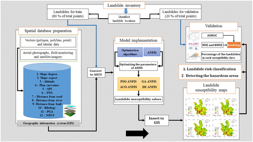
As stated earlier, in this paper we utilized the combination of the ANFIS models with four robust optimization techniques, namely PSO, GA, ACO, and DE for analyzing the occurrence risk of landslide triggered earthquake in the Ludian County of China. To this end, after preparing the proper database, the proposed predictive methods were implemented to estimate the landslide susceptibility index. Figure 4 portrays the procedure we carried out to achieve the landslide susceptibility map. The description of the ANFIS, PSO algorithm, GA algorithm, ACO algorithm, and DE algorithm are presented in this section.

Figure 4. Graphical methodology of applied procedure for landslide susceptibility zonation.

4.1. Adaptive neuro-fuzzy inference system (ANFIS)

Recently, the fuzzy theory has widely gained attention by researchers due to its ability for displaying complex processes by employing the concepts and if-then rules. The fuzzy theory is inspired by the concept of decision making in human life. However, it should be mentioned that preferable results are not offered for unforeseen situations by this algorithm (Dehnavi et al. 2015). Thus, to take on a self-learner property, the artificial neural network (ANN) has been utilized to optimize the fuzzy theory as ANFIS. Jang (1993) has proposed ANFIS as a hybrid of ANN and a fuzzy system. To solve nonlinear problems, it can be mentioned that the ANFIS offers better results than a fuzzy inference system (FIS). According to the ANFIS, a FIS is employed for training in a multilayer feed-forward network (Dixon 2005). By combining least-squares methods and back-propagation gradient descent, FIS membership function (MF) parameters can be trained through training the input data by the ANFIS. As Figure 5 illustrates, in the ANFIS model, the layers are structured as follows (Termeh et al. 2018):

Figure 5. Typical ANFIS structure.

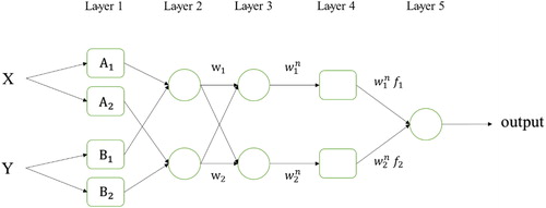
Each node in layer 1 contains adaptive nodes as: (3) $$O_{1,i}=\mu A_i\left(x\right)$$(3) (4) $$O_{1,i}=\mu B_i\left(y\right)$$(4) where $x\hspace{0.17em}\text{and}\hspace{0.17em}y$ symbolize the input nodes. $A\hspace{0.17em}\text{and}\hspace{0.17em}B$ indicate the linguistic variables, and $\mu A_i(x)\hspace{0.17em}\text{and}\hspace{0.17em}\mu B_i(y)$ represent the MFs of the proposed node. In the second layer, Equation (5)(5) $$O_{2,i}=W_i=\mu A_i\left(x\right)\mu B_i\left(y\right),i=1.2$$(5) expresses the output of each node which is the outcome of all input signals to the proposed node. (5) $$O_{2,i}=W_i=\mu A_i\left(x\right)\mu B_i\left(y\right),i=1.2$$(5) where $W_i$ indicates the product of each node.

The normalized outputs of layer 2 are considered as the nodes of layer 3. (6) $$O_{3,i}={\overline{w}}_l=\frac{w_i}{w_1+w_2},i=1.2$$(6)

For layer 4, a node function is employed to associate each node as follows: (7) $$O_{4,i}={\overline{w}}_l{f}_i={\overline{w}}_l\left(p_{i}x+q_{i}y+r_i\right)$$(7) where ${\overline{w}}_l$ represents the normalized firepower of layer 3, and $p_i,q_i,\hspace{0.17em}\text{and}\hspace{0.17em}{r}_i$ denote the node parameters. In layer 4, the parameters are considered as the result parameters.

The sum of all input signals and all the way to the output is considered as a single node of layer 5. (8) $$O_{5,i}=\sum {\overline{w}}_l{f}_i=\sum w_i{f}_i/\sum w_i,i=1.2$$(8)

4.2. Particle swarm optimization (PSO) algorithm

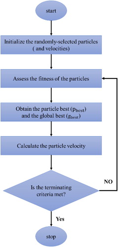
During the past several decades, improving the optimization approaches based on particle intelligence technique has increasingly gained attention by a number of researchers because of its potential for modelling the real-life swarm behaviours such as bird-flocking, fish-schooling, etc. Due to the high run strength and flexibility, the PSO has always been amongst researchers’ top priorities for many issues and has been employed for many nonlinear-continuous and discrete systems (Kennedy 2010; Bui et al. 2017a). Figure 6 exhibits the flowchart of the PSO technique. In this model, a population of random solutions is considered for the system; subsequently, by updating generations, the system searches for optima. Therefore, it should be mentioned that the PSO algorithm shares many similarities with conventional optimization methods. However, unlike evolutionary computation techniques, the position of particles depends on their velocity parameter (step motor) according to the PSO algorithm.

Figure 6. The simple flowchart of the PSO algorithm.

Based on the PSO algorithm, each particle possesses a utility function and a speed vector which signify its orientation and step, respectively (Clerc and Kennedy 2002). Each particle moves in the search space, and the position of its previous best position and velocity has been kept as a record. By considering its own moving experience, the velocity and position of each particle are dynamically updated in the evolution of each generation. Thus, each particle goes to a better location, and the optimal solution is determined for the system. For each particle, the mathematical expression for updating the velocity is presented by the following equation. (9) $$V_{\mathit{ij}}(t+1)=W\ast V_{\mathit{ij}}\left(t\right)+r_1*c_1\left(p_{\mathit{ij}}\left(t\right)-x_{\mathit{ij}}\left(t\right)\right)+r_2*c_2\left(g_i\left(t\right)-x_{\mathit{ij}}\left(t\right)\right)$$(9) where $p_{\mathit{ij}}(t)\hspace{0.17em}\text{and}\hspace{0.17em}{g}_i(t)$ stand for the best total personal experience and the most proper cumulative experience, respectively. $W$ indicates the inertia coefficient which illustrates the tendency of a parameter for balance. $c_1\hspace{0.17em}\text{and}\hspace{0.17em}{c}_2$ represent the personalized coefficient learning and the collective learning coefficient, respectively. In addition, and $r_1\hspace{0.17em}\text{and}\hspace{0.17em}{r}_2$ denote uniform random numbers which can range between 0 and 1. By considering the updated velocity of each particle, the new particle position can be obtained by Equation (10)(10) $$X(t+1)=X\left(t\right)+V(t+1)$$(10) : (10) $$X(t+1)=X\left(t\right)+V(t+1)$$(10)

Consequently, for the next stage, the particle position and new particle velocity are updated according to the above equation.

4.3. Genetic algorithm (GA)

To solve learning processes and optimization problems in different fields, GA has been utilized by the researchers as a heuristic algorithm. This algorithm is inspired by Darwin’s evolution theory as well as biological evolution in nature (Sheta and Turabieh 2006). Holland (1975) has introduced the GA, and then it has been developed. In this algorithm, the structure is composed of a population, and each individual of the population, called chromosome, is considered as a solution to the problem. Different problem variables act as genes for an individual in this algorithm (Mitchell 1998). Figure 7 depicts the mechanism of this method. According to GA, a random population of chromosomes is developed in order to create the search procedure. Subsequently, three operators produce the next generation of the population as follows:

Figure 7. The overall flowchart of the GA algorithm (Moayedi et al. 2019a).

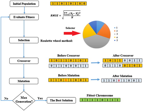
Selection Operator: Based on this operator, the fitness function of each chromosome is calculated, and the obtained results are evaluated in each stage. Consequently, the best solutions to the problem are identified as the best chromosomes of society. Furthermore, to produce the next generation, the chromosomes are employed as parents; therefore, new child chromosomes are produced as offspring. It is worth noting that better chromosomes have a higher chance of combining with other individuals.

Crossover Operator: According to this operator, the combined selected chromosomes have been used; therefore, the new child chromosomes have better fitness than its parents. Thus, the ratio and structure of the offspring’s chromosome compared with its parents’ chromosomes have been determined by employing the crossover operator. Various methods, including Uniform, Cycle, N-Point, Tournament, Order, Ranking Selection, and partially mapped can be employed for implementing the crossover operator (Saeidian et al. 2016). In this study, the uniform method has been employed for this issue.

Mutation Operator: Searching new areas has been carried out in the available dimension based on this operator. A mutation is produced in the chromosome by changing one or more genes inside the chromosomes randomly. Thus, the value of the selected gene is changed by selecting a chromosome for mutation. It should be mentioned that the mutation operator is employed for applying to either a terminal node (variables and constants) or a function node (arithmetic operations) (Nourani et al. 2014).

By employing these three operators, new child chromosomes are produced and they are considered as the next generation parents. In addition, the trend goes on in order to the termination condition is met.

4.4. Ant colony optimization (ACO) algorithm

As a multi-criteria technique, Dorigo and Blum (2005) have proposed the ant algorithm for solving optimization problems, including travelling salesman. The ant algorithm has been introduced by considering a principle that collective clever behaviour is achieved by local simple and confined interactions of members or class of the population. The speed and parallel performance, distributed creatures’ transactions, and lack of centralized control can be mentioned as the main superiority of collective intelligence (Beckers et al. 1992). According to the ant algorithm, the trail of different pheromones is left along the path by the ants, and they help each other for choosing the shortest path. For an n-dimension space, a route between $X_i\hspace{0.17em}\text{and}\hspace{0.17em}{X}_j\hspace{0.17em}\left(\text{or}\hspace{0.17em}{Y}_i\hspace{0.17em}\text{and}\hspace{0.17em}{Y}_j\right)$ has the probability of selecting by an ant q as follows (Beckers et al. 1992): (11) $$P_{\mathit{ij}}^q\left(t\right)=\{\begin{array}{c}\frac{{\tau }_{\mathit{ij}}^{\alpha }\left(t\right)\ast {\eta }_{\mathit{ij}}^{\beta }\left(t\right)}{{\sum }_{u\in N_i^q}{\tau }_{\mathit{iu}}^{\alpha }\left(t\right)\ast {\eta }_{\mathit{iu}}^{\beta }\left(t\right)}\\ 0 j\notin N_i^q\end{array}$$(11) where ${\tau }_{\mathit{ij}}(t),t,{\eta }_{\mathit{ij}}(t),\hspace{0.17em}\mathrm{and}\hspace{0.17em}{N}_i^q$ indicate the pheromone intensity, the time, the value of cost function between the points $i\hspace{0.17em}\text{and}\hspace{0.17em}j$, and the sum of point $i$ and neighbours of the ant $q$, respectively. In addition, the cost function and weight of pheromone intensity have been determined by the control parameters $\beta \hspace{0.17em}\text{and}\hspace{0.17em}\alpha$, respectively. In the real world, each ant follows paths with more pheromones which have been secreted by other ants in their way back to the nest. Thus, the ants choose a shorter route which has more pheromones because its pheromones are strengthened faster than the pheromones of a longer path. According to the ant algorithm, the process of finding the best solution is based on the mentioned action of ants. The learning of model and evaluating the selected route through back and forth trial are inspired by the mentioned action. For an ant $q$, $P_{\mathit{ij}}^q(t)$ denotes the probability of transferring from the point $i\hspace{0.17em}\text{to}\hspace{0.17em}j$ in $t$ the iteration. If a point has not been visited by an ant, $P_{\mathit{ij}}^q(t)$ is zero, and $j\notin N_i^q$.

Equation (12)(12) $${\tau }_{\mathit{ij}}(t+1)=\left(1-\rho \right).{\tau }_{\mathit{ij}}\left(t\right)+\rho .{\tau }_0$$(12) formulates the intensity of pheromone is upgraded for selecting a new route: (12) $${\tau }_{\mathit{ij}}(t+1)=\left(1-\rho \right).{\tau }_{\mathit{ij}}\left(t\right)+\rho .{\tau }_0$$(12) where $\rho \hspace{0.17em}\text{and}\hspace{0.17em}{\tau }_0$ denote the evaporation intensity of pheromone and the pheromone’s initial value, respectively.

The error probability of choosing a shorter route by ants can be increased for an attractive route because its food may end, but the remaining pheromones are still present on the track. Consequently, the pheromone intensity is refreshed at the end of each iteration by the following formulation: (13) $$\{\begin{array}{ll}{\tau }_{\mathit{ij}}(t+1)=\left(1-\rho \right).& {\tau }_{\mathit{ij}}\left(t\right)+\rho .\Delta {\tau }_{\mathit{ij}}\left(t\right)\\ \Delta {\tau }_{\mathit{ij}}\left(t\right)=\frac{Q}{L^k\left(t\right)}& \text{if}\left(i,j\right)\in \text{best}\hspace{0.17em}\text{created}\hspace{0.17em}\text{tour}\\ 0& \text{else}\end{array}$$(13) where $\Delta {\tau }_{\mathit{ij}}(t),Q,\hspace{0.17em}\mathrm{and}\hspace{0.17em}{L}^k(t)$ represent the amount of pheromone added to ${\tau }_{\mathit{ij}}$ by ants, the constant parameter, and the optimal value of cost function, respectively.

4.5. Differential evolutionary (DE) algorithm

Recently, as another widely used evolution algorithm, the DE algorithm has been employed to find the globally optimal solution for a problem with continuous space (Storn and Price 1997; Storn 2008; Das et al. 2009). Storn and Price (1997) have proposed the DE algorithm which the next optimal generation is produced by three operators, including, mutation, crossover, and selection. By producing a random population, the DE algorithm starts its operation, and each individual is considered as a symbol of a solution for the problem. The vector $X_i^G=(x_{1,i}^G,x_{2,i}^G,x_{3,i}^G,\dots ,x_{D,i}^G)$ stands for an individual of the population and $i=\{0,1,2,\dots ,\mathit{NP}\}$ indicates the number of the mentioned individual in the population. $\mathrm{D}$ denotes the search dimension (i.e. the number of components in a problem). $G=\{0,1,2,\dots ,G_{\max }\}$ is the generation times in which $G_{\max }$ shows the total number of produced generations. By supposing $X_L=\{x_{1,L},x_{2,L},x_{3,L},\dots ,x_{D,L}\}$ and $X_U=11$ as the lower and upper limits of each search dimension, the initial population can be defined as Equation (14)(14) $$x_{j,i}^0=x_{j,L}+\text{rand}\left(0.1\right).\left(x_{j,U}-x_{j,L}\right)$$(14) : (14) $$x_{j,i}^0=x_{j,L}+\text{rand}\left(0.1\right).\left(x_{j,U}-x_{j,L}\right)$$(14) where $\text{rand}(0.1)$ represents a uniformly distributed random number in [0,1].

Mutation: As the first operator of DE algorithm, the mutation operator employs each individual, called the target vector $X_i^G$, to produce the mutant vector (donor vector) $V_i^G=\left(V_1^G,V_2^G,V_3^G,\dots ,V_D^G\right)$ as follows (Abdul-Rahman et al. 2013; Zheng et al. 2014): (15) $$\begin{array}{c}\text{DE}/\text{rand}/1:V_i^G=X_{r1}^G+F.\left(X_{r2}^G-X_{r3}^G\right)\\ \text{DE}/\text{rand}/2:V_i^G=X_{r1}^G+F.\left(X_{r2}^G-X_{r3}^G\right)+F.\left(X_{r4}^G-X_{r5}^G\right)\\ \text{DE}/\mathrm{best}/1:V_i^G=X_{\mathit{best}}^G+F.\left(X_{r1}^G-X_{r2}^G\right)\\ \text{DE}/\mathrm{best}/2:V_i^G=X_{\mathit{best}}^G+F.\left(X_{r1}^G-X_{r2}^G\right)+F.\left(X_{r3}^G-X_{r4}^G\right)\\ \text{DE}/\mathrm{current}-\mathrm{to}-\text{rand}/1:V_i^G=X_i^G+F.\left(X_{r1}^G-X_i^G\right)+F.\left(X_{r2}^G-X_{r3}^G\right)\\ \text{DE}/\mathrm{current}-\mathrm{to}-\text{best}/1:V_i^G=X_i^G+F.\left(X_{\mathit{best}}^G-X_i^G\right)+F.\left(X_{r1}^G-X_{r2}^G\right)\end{array}$$(15) where $r1,r2,r3,\hspace{0.17em}\text{and}\hspace{0.17em}r4$ indicate random integers from [0, NP] in which $r1\ne r2\ne r3\ne r4$. $F$ symbolizes a number that is randomly chosen from [0, 1] and denotes a scale factor that defines the mutation scale. $X_{\mathit{best}}^G$ presents an individual who will have the most appropriate fitness value in the generation population.

Crossover: Producing the trial vector $U_{j,i}^G=\left\{u_{1,i}^G,u_{2,i}^G,u_{3,i}^G,\dots ,u_{D,i}^G\right\}$ is the aim of the crossover operator. Therefore, some relations of the target vector $X_i^G$ are replaced with the mutant vector $V_i^G$ in order to achieve this goal. The crossover operator can be formulated by Equation (16)(16) $$U_{\mathit{ji}}^G=\{\begin{array}{ll}{V}_{\mathit{ji}}^G& \text{if}\text{rand}\left[0.1\right]\le \mathit{CR}\mathrm{or}j=j_{\text{rand}}\\ X_{\mathit{ji}}^G& \text{otherwise}\end{array}$$(16) (Storn and Price 1997): (16) $$U_{\mathit{ji}}^G=\{\begin{array}{ll}{V}_{\mathit{ji}}^G& \text{if}\text{rand}\left[0.1\right]\le \mathit{CR}\mathrm{or}j=j_{\text{rand}}\\ X_{\mathit{ji}}^G& \text{otherwise}\end{array}$$(16) where $i\in \left\{1,2,3,\dots ,\text{NP}\right\}\hspace{0.17em}\text{and}\hspace{0.17em}j\in \left\{1,2,3,\dots ,D\right\}$. $j_{\text{rand}}$ denotes a random number in [1, D]. $\mathit{CR}$ is uniformly distributed at random in [0, 1] and indicates the crossover rate.

Selection: According to this operator, the best choice is determined for the next generation by comparing the fitness value of the trial vector $U_i^G$ with the target vector $X_i^G$ as follows (Storn and Price 1997): (17) $$X_i^{G+1}=\{\begin{array}{ll}{U}_i^G& \text{if}f\left(U_i^G\right)\le f\left(X_i^G\right)\\ X_i^G& \text{otherwise}\end{array}$$(17)

5. Results and discussion

In this paper, using the programming software of MATLAB version 14.0 and ArcGIS version 10.2 we developed four optimization techniques, namely PSO, GA, ACO, and DE, synthesized with ANFIS for analyzing the earthquake-triggered landslide risk. The Ludian County of China was selected as the study area, due to the Ludian earthquake occurred in 2014 which caused several slope failures in this region. Notably, we considered 12 landslide causative factors (namely, elevation, slope degree, lithology, PGA, SPI, TWI, distance to road, distance to river, distance to fault, NDVI, slope aspect, and plan curvature) to produce the spatial database. In this sense, factors with basic formats (point, polygon, polyline) were converted to GIS rasters. Also, 80% of landslide points (i.e. 366 landslides) devoted to the training process, and the remaining 20% (i.e. 92 landslides) were used to validate the performance of PSO-ANFIS, ACO-ANFIS, GA-ANFIS, and DE-ANFIS models.

In the context of model performance, PSO, GA, ACO, and DE metaheuristic algorithms were coded to fine-tuning the parameters of ANFIS MFs (Mahapatra et al. 2015). More specifically, when the algorithm starts, a basic fuzzy system is generated using the received training data. Next, among the stored basic parameters, the optimization algorithms select the best ones according to a predefined objective function (OF). An example of the optimized ANFIS structure is illustrated in Figure 8.

Figure 8. Flowchart of the optimized structure of ANFIS.

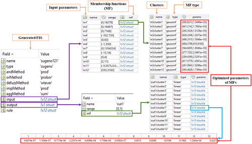
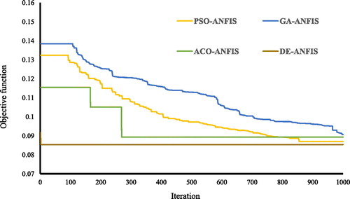
In this study, we used mean square error (MSE) as the OF which is defined by Equation (18)(18) $$\mathit{MSE}=\frac{1}{N}{\sum _{i=1}^N(Y_{i_{\mathit{observed}}}-Y_{i_{\mathit{predicted}}})}^2$$(18) : (18) $$\mathit{MSE}=\frac{1}{N}{\sum _{i=1}^N(Y_{i_{\mathit{observed}}}-Y_{i_{\mathit{predicted}}})}^2$$(18) where N is the number of instances, and Y_{i observed}, and Y_{i predicted} denote the target data and predicted values of landslide susceptibility index, respectively. Each model performed within 1000 repetitions. The convergence curves of the designed models are depicted in Figure 9 in term of MSE. According to this chart, DE-ANFIS yielded the converged solution in the first iteration that indicates the highest convergence speed. The ACO-ANFIS reached the lowest value of the OF after 271 iterations. This is while, the ensembles of PSO-ANFIS and GA-ANFIS kept the optimization until the 858^th and the latest iteration, respectively.

Figure 9. The convergence curves of the OFs for the used models.

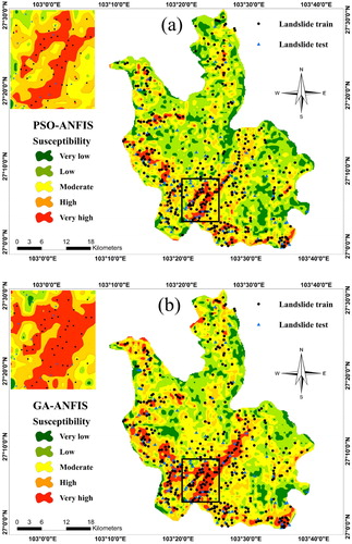
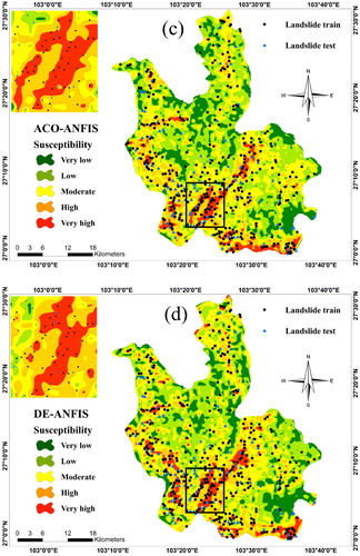
Then, the proposed ensemble methods were implemented to calculate the landslide susceptibility index. The landslide susceptibility maps were generated by transferring the outputs into the ArcGIS environment. Then, a natural break classification (Akgun et al. 2012; Xu et al. 2012; Pourghasemi et al. 2013; Jaafari et al. 2014) was applied to stratify the resulted maps into five susceptibility groups namely, ‘Very low’, ‘Low’, ‘Moderate’, ‘High’, and ‘Very high’. Figure 10 depicts the classified susceptibility maps obtained from the PSO-ANFIS, ACO-ANFIS, GA-ANFIS, and DE-ANFIS predictions.

Figure 10. Landslide susceptibility map developed by (a) PSO-ANFIS, (b) ACO-ANFIS, (c) GA-ANFIS, and (d) DE-ANFIS models.

The statistical report from the performance of the applied models are presented in Figure 11 for both training and testing phases based on the (i) comparison between the targets and outputs, (ii) MSE and RMSE value of data, and (iii) frequency errors of data samples. In addition, Figure 12 illustrates the ROC curve we depicted in SPSS environment for each ensemble model. This diagram shows the true positive rate (on the vertical axis) against the false positive rate (on the horizontal axis) of the model’s estimations. Remarkably, the AUROC criterion represents the accuracy of the proposed prediction so that a casual prediction is determined by 0.5, and 1 indicates an ideal estimation.

Figure 11. The results obtained for (a and b) PSO-ANFIS, (c and d) GA-ANFIS, (e and f) ACO-ANFIS, and (g and h) DE-ANFIS prediction, respectively for the training and testing samples.

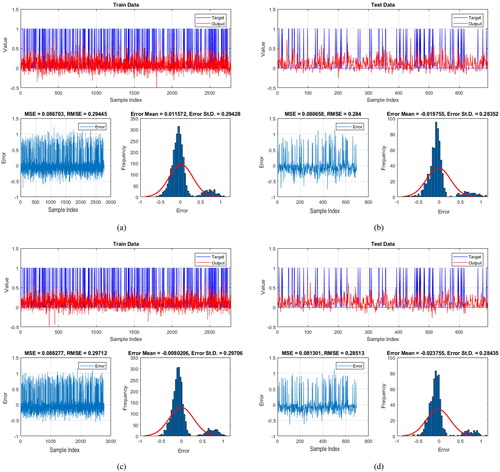
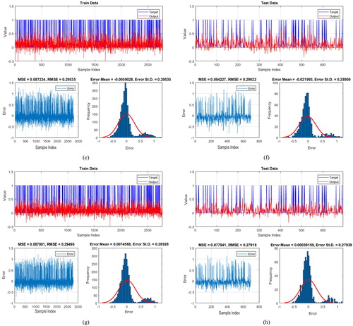
Figure 12. The ROC diagram, obtained for (a) PSO-ANFIS, (b) GA-ANFIS, (c) ACO-ANFIS, and (d) DE-ANFIS prediction.

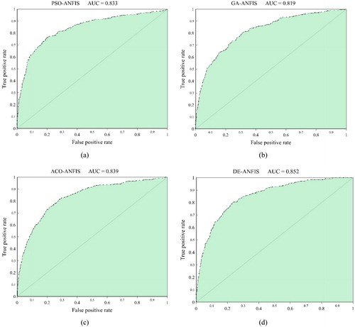
Referring to Figures 11 and 12, a satisfying performance rate can be concluded for all developed methods. The MSE criterion computed for the training (0.086, 0.088, 0.087, and 0.087, respectively for PSO-ANFIS, GA-ANFIS, ACO-ANFIS, and DE-ANFIS) and testing (0.080, 0.081, 0.084, and 0.077) datasets reveal that compared to the training phase, all designed models have shown a better approximation in testing dataset. Also, PSO-ANFIS (MSE_train = 0.086) and DE-ANFIS (MSE_test = 0.077) gave the outputs with the lowest MSE in training and testing phases, respectively. Considering the training RMSE, the most effective learning commonly emerges for PSO-ANFIS and DE-ANFIS (RMSE_train = 0.294) followed by ACO-ANFIS (RMSE_train = 0.295) and GA-ANFIS (RMSE_train = 0.297). Moreover, similar to testing MSE, the lowest and highest-testing RMSE is acquired for DE-ANFIS (RMSE_train = 0.279) and ACO-ANFIS (RMSE_test = 0.290). Besides, based on Figure 12, the best prediction of the landslide susceptibility index was carried out by DE-ANFIS with 85.2% accuracy. The second-accurate model was ACO-ANFIS (AUROC = 0.839) followed by PSO-ANFIS (AUROC = 0.833) and GA-ANFIS (AUROC = 0.819).

Table 2 denotes the ranking system developed based on the values calculated for MSE, RMSE, and AUROC. According to this table, each predictive model gains a total ranking score (TRS) which determines the final rank of each model. In this sense, the total scores of 15, 8, 10, and 18, respectively acquired for PSO-ANFIS, GA-ANFIS, ACO-ANFIS, and DE-ANFIS methods demonstrate that the combination of adaptive neuro-fuzzy inference system and DE algorithm suggests the most robust method for the assessment of earthquake-induced landslide hazard. After that, PSO-ANFIS outperforms the ACO-ANFIS and GA-ANFIS which have featured as the models with gratifying accuracy.

Table 2. The ranking system based on the results of the spatial prediction of landslide susceptibility.

Ensemble models	Network results					Ranking score					Total ranking score (TRS)	Rank
	Training phase		Testing phase		AUROC	Training phase		Testing phase		AUROC
	MSE	RMSE	MSE	RMSE		MSE	RMSE	MSE	RMSE
PSO-ANFIS	0.086	0.294	0.080	0.284	0.833	4	3	3	3	2	15	2
GA-ANFIS	0.088	0.297	0.081	0.285	0.819	2	1	2	2	1	8	4
ACO-ANFIS	0.087	0.295	0.084	0.290	0.839	3	2	1	1	3	10	3
DE-ANFIS	0.087	0.294	0.077	0.279	0.852	3	3	4	4	4	18	1

Based on the results, the combination of the used fuzzy-based tool with evolutionary algorithms can perform efficiently for the purpose of landslide susceptibility mapping. Putting a detailed comparison between various ensembles of ANFIS aside, the greatest achievement of this research lies in presenting an accurate and inexpensive evaluative approach for spatial assessment of earthquake induced-landslide hazard. In addition, due to the high speed of the DE-ANFIS in the convergence, the quickness of this model can be mentioned as an advantage in comparison with other intelligent and statistical-based approaches.

In comparison with previous studies that developed the susceptibility map for the landslides triggered by the Ludian earthquake, the results of this study are more satisfying. In details, as explained, Li et al. (2017) generated the landslide susceptibility map of the Ludian along with two other study areas, by designing a GA and a novel GA models for proper selection of conditioning factors, which led to 82.21% and 82.28% accuracy of the results for the Ludian, respectively. However, the GA-based ensemble of our study performed worse than their models, other three ensembles of PSO-ANFIS, ACO-ANFIS, and DE-ANFIS outperformed those. Moreover, Tian et al. (2017) investigated the susceptibility analysis of the pre-earthquake and coseismic landslides (immediately after the earthquake) related to the mentioned earthquake, in the southern part of the Ludian. They used the Information value method in that study. The AUC-based accuracy for the spatial risk analysis of the coseismic landslides was 77.05%. As is seen, the accuracy of all four methods we used in this study is considerably higher than this value. This is noteworthy that they considered only seven landslide-related factors, namely slope angle, elevation, slope aspect, distance from drainages, intensity, curvature, and lithology, while we used five more factors. Along with the higher potential of the used employed models, it may be a reason for more accuracy of our research.

Furthermore, in comparison with the studies that used the same methods for the landslide susceptibility mapping in different areas, it was revealed that the main results of this study are more accurate. In Xie et al. (2017), for instance, they used ANFIS-PSO, ANFIS-DE, and ANFIS-GA for landslide hazard assessment in Hanyuan County of China. In term of AUROC, the ANFIS-DE was found the best model with 0.844, followed by ANFIS-GA with 0.821, and ANFIS-PSO with 0.780. As is seen, however their GA-based ensemble performed slightly better than ours’, the PSO-ANFIS (AUROC = 0.833) and DE-ANFIS (AUROC = 0.852) of this study present a more reliable prediction. Notably, in term of the MSE and RMSE, all three methods of the present research showed a more efficient performance. Other than some differences between the used conditioning factors, the considered ratio for the division of the marked landslides (i.e. into the training and testing datasets) may be another influential factor. This ratio was determined as 80:20 and 70:30 in the present study and (Xie et al. 2017).

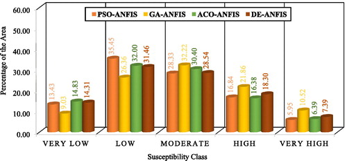
For more details, the percentages of landslide susceptibility classes are presented in the form of a column chart in Figure 13. As the chart illustrates, 13.43%, 9.03%, 14.83%, and 14.31% of the studied area is located in the very low susceptibility class, respectively by PSO-ANFIS, GA-ANFIS, ACO-ANFIS, and DE-ANFIS ensembles. Likewise, respective proportions of 35.45%, 26.36%, 32.00%, and 31.46% of the Ludian County are distinguished by the low risk of earthquake-induced landslides. All designed ensembles have detected close ratios (between 28% and 33%) of the intended region for the moderate susceptibility class. As for the dangerous areas, about 22.80%, 32.40%, 22.80%, and 25.70% of the Ludian district is under the high and very high landslide occurrence risk, respectively based on the PSO-ANFIS, GA-ANFIS, ACO-ANFIS, and DE-ANFIS predictions.

Figure 13. Column chart showing the percentage of landslide susceptibility classes over the study area.

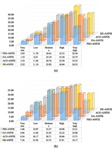
In the following, a novel idea was performed to calculate the percentage of the training and testing landslides located in each susceptibility class. To do this, we crossed the landslide layers with the generated susceptibility maps. The results of this process are shown by 3D bar charts in Figure 14(a,b) for the training and validation landslide points. According to these charts, GA-ANFIS has categorized the greatest percentage of the identified landslides (32.75% and 25.88%, respectively for the training and testing records) in very high susceptibility class. In a glance, it can be induced that the highest and lowest density of the landslide locations in both datasets observed within the high and very low susceptibility classes, respectively. The ACO-ANFIS ensemble has stratified approximately 12% and 29% of the training landslides in low and moderate susceptibility classes which are the greatest proportions in the mentioned classes. Investigating the results of the elite models, i.e. DE-ANFIS and PSO-ANFIS, about 58% and 63% of the training landslides and also 46% and 43% of the landslides devoted to the validation phase were located in perilous regions of the Ludian County (high and very high categories).

Figure 14. The 3D bar charts showing the percentage of the (a) training and (b) testing landslides located in each susceptibility classes.

6. Conclusions and remarks

Due to the crucial role of the landslide susceptibility mapping in hazard mitigation, this study deals with the application of ensembles of ANFIS with four metaheuristics techniques, namely PSO, GA, ACO, and DE algorithm for analyzing the occurrence likelihood of earthquake-induced landslide in Ludian County, China. To achieve this aim, 12 landslide-related factors, namely: elevation, slope degree, lithology, PGA, SPI, TWI, distance to road, distance to river, distance to fault, NDVI, slope aspect, and plan curvature were taken into consideration within the GIS. Also, the landslide inventory map was composed of 458 earthquake-induced landslides. Among those, 366 (80%) landslides were devoted to the learning process, and the remaining 92 (20%) were used to evaluate the accuracy of results. Three well-known accuracy criteria of MSE, RMSE, and AUROC were used to develop a ranking system to compare the usefulness of the applied models. The following conclusions were obtained based on the results. It shall be noted that, to have a coherent presentation of the results, calculated values of MSE, RMSE, and AUROC have been reported in the respective order for PSO-ANFIS, GA-ANFIS, ACO-ANFIS, and DE-ANFIS in all cases.

• The convergence rate of the applied models showed that the DE-ANFIS is the fastest ensemble which achieved the optimum solution after the first iteration. The ACO-ANFIS and PSO-ANFIS were found to be the second and third quick models, due to reaching the lowest OF after 271 and 858 iterations, respectively. This is while, GA-ANFIS kept decreasing the error till the 1000th iteration.

• All four ensembles of PSO-ANFIS, GA-ANFIS, ACO-ANFIS, and DE-ANFIS have presented an effective approximation of the landslide hazard, due to the acquired values of accuracy criteria.

• Based on the MSEs computed for training (0.086, 0.088, 0.087, and 0.087) and testing (0.080, 0.081, 0.084, and 0.077) phases, the DE-ANFIS has shown the best performance in the validation phase. Also, the PSO algorithm outperformed GA and ACO for enhancing the prediction capability of ANFIS. In term of RMSE, the training error values (0.294, 0.297, 0.295, and 0.294) indicate the superiority of PSO-ANFIS and DE-ANFIS with equal RMSEs. Likewise, the RMSE of the testing samples (0.284, 0.285, 0.290, and 0.279) shows that the highest and lowest RMSEs are obtained for ACO-ANFIS and DE-ANFIS, respectively.

• The calculated AUROCs report 83.3%, 81.9%, 83.9%, and 85.2% accuracy for the designed systems. Unlike the MSE and RMSE, ACO-ANFIS performed slightly better than PSO-ANFIS. However, similar to prior conclusions, DE improved ANFIS more efficiently compared to the other three techniques.

• All in all, based on the acquired TRSs, DE-ANFIS (TRS = 18) was found to be the most capable algorithm in this research, followed by PSO (TRS = 15), ACO-ANFIS (TRS = 10), and GA-ANFIS (TRS = 8).

• Classifying the study area into five landslide susceptibility groups, it was revealed that about 22.80%, 32.40%, 22.80%, and 25.70% of the Ludian district is under the high and very high landslide occurrence risk.

• Last but not least, analyzing the distribution of the identified landslides, it was concluded that 63%, 66%, 56%, and 58% of the training landslides, and also 43%, 58%, 45%, and 46% of the testing landslides were located in the perilous areas of the Ludian.

Disclosure statement

No potential conflict of interest was reported by the authors.

Additional information

Funding

This research was supported by Ton Duc Thang University (Vietnam).

References

- Abdul-Rahman OA, Munetomo M, Akama K. 2013. An adaptive parameter binary-real coded genetic algorithm for constraint optimization problems: performance analysis and estimation of optimal control parameters. Inf Sci. 233:54–86.
- Ahmadlou M, Karimi M, Alizadeh S, Shirzadi A, Parvinnejhad D, Shahabi H, Panahi M. 2018. Flood susceptibility assessment using integration of adaptive network-based fuzzy inference system (ANFIS) and biogeography-based optimization (BBO) and BAT algorithms (BA). Geocarto Int.:1–21.
- Akgun A, Sezer EA, Nefeslioglu HA, Gokceoglu C, Pradhan B. 2012. An easy-to-use MATLAB program (MamLand) for the assessment of landslide susceptibility using a Mamdani fuzzy algorithm. Comput Geosci. 38:23–34.
- Beckers R, Deneubourg J-L, Goss S. 1992. Trails and U-turns in the selection of a path by the ant Lasius niger. J Theor Biol. 159(4):397–415.
- Beven KJ, Kirkby MJ. 1979. A physically based, variable contributing area model of basin hydrology/Un modèle à base physique de zone d’appel variable de l’hydrologie du bassin versant. Hydrol Sci J. 24(1):43–69.
- Binh Thai P, Dieu Tien B, Prakash I. 2018a. Bagging based support vector machines for spatial prediction of landslides. Environ Earth Sci. 77:146.
- Binh Thai P, Indra P, Dieu Tien B. 2018b. Spatial prediction of landslides using a hybrid machine learning approach based on random subspace and classification and regression trees. Geomorphology. 303:256–270.
- Binh Thai P, Prakash I, Jaafari A, Dieu Tien B. 2018c. Spatial prediction of rainfall-induced landslides using aggregating one-dependence estimators classifier. J Indian Soc Remote Sens. 46:1457–1470.
- Bui DT, Bui Q-T, Nguyen Q-P, Pradhan B, Nampak H, Trinh PT. 2017a. A hybrid artificial intelligence approach using GIS-based neural-fuzzy inference system and particle swarm optimization for forest fire susceptibility modeling at a tropical area. Agric Forest Meteorol. 233:32–44.
- Bui DT, Tuan TA, Hoang N-D, Thanh NQ, Nguyen DB, Van Liem N, Pradhan B. 2017b. Spatial prediction of rainfall-induced landslides for the Lao Cai area (Vietnam) using a hybrid intelligent approach of least squares support vector machines inference model and artificial bee colony optimization. Landslides. 14:447–458.
- Bui DT, Tuan TA, Klempe H, Pradhan B, Revhaug I. 2016. Spatial prediction models for shallow landslide hazards: a comparative assessment of the efficacy of support vector machines, artificial neural networks, kernel logistic regression, and logistic model tree. Landslides. 13:361–378.
- Chen W, Chai H, Sun X, Wang Q, Ding X, Hong H. 2016. A GIS-based comparative study of frequency ratio, statistical index and weights-of-evidence models in landslide susceptibility mapping. Arab J Geosci. 9(3):204.
- Chen W, Panahi M, Khosravi K, Pourghasemi HR, Rezaie F, Parvinnezhad D. 2019a. Spatial prediction of groundwater potentiality using ANFIS ensembled with teaching-learning-based and biogeography-based optimization. J Hydrol. 572:435–448.
- Chen W, Panahi M, Tsangaratos P, Shahabi H, Ilia I, Panahi S, Li S, Jaafari A, Ahmad BB. 2019b. Applying population-based evolutionary algorithms and a neuro-fuzzy system for modeling landslide susceptibility. Catena. 172:212–231.
- Chen W, Pourghasemi HR, Panahi M, Kornejady A, Wang J, Xie X, Cao S. 2017. Spatial prediction of landslide susceptibility using an adaptive neuro-fuzzy inference system combined with frequency ratio, generalized additive model, and support vector machine techniques. Geomorphology. 297:69–85.
- Chen W, Shahabi H, Shirzadi A, Hong H, Akgun A, Tian Y, Liu J, Zhu A-X, Li S. 2018a. Novel hybrid artificial intelligence approach of bivariate statistical-methods-based kernel logistic regression classifier for landslide susceptibility modeling. Bull Eng Geol Environ.:1–23.
- Chen W, Shahabi H, Zhang S, Khosravi K, Shirzadi A, Chapi K, Pham B, Zhang T, Zhang L, Chai H, et al. 2018b. Landslide susceptibility modeling based on GIS and novel bagging-based kernel logistic regression. Appl Sci. 8(12):2540.
- Chen W, Tsangaratos P, Ilia I, Duan Z, Chen X. 2019c. Groundwater spring potential mapping using population-based evolutionary algorithms and data mining methods. Sci Total Environ. 684:31–49.
- Chen W, Zhao X, Shahabi H, Shirzadi A, Khosravi K, Chai H, Zhang S, Zhang L, Ma J, Chen Y. 2019d. Spatial prediction of landslide susceptibility by combining evidential belief function, logistic regression and logistic model tree. Geocarto Int.:1–25.
- Cheng J, Wu Z, Liu J, Jiang C, Xu X, Fang L, Zhao X, Feng W, Liu R, Liang J, Yang T. 2015. Preliminary report on the 3 August 2014, M w 6.2/M s 6.5 Ludian, Yunnan–Sichuan border, southwest China, earthquake. Seismol Res Lett. 86(3):750–763.
- Clerc M, Kennedy J. 2002. The particle swarm-explosion, stability, and convergence in a multidimensional complex space. IEEE Trans Evol Comput. 6(1):58–73.
- Das S, Abraham A, Chakraborty UK, Konar A. 2009. Differential evolution using a neighborhood-based mutation operator. IEEE Trans Evol Comput. 13(3):526–553.
- Dehnavi A, Aghdam IN, Pradhan B, Varzandeh M, Morshed H. 2015. A new hybrid model using step-wise weight assessment ratio analysis (SWARA) technique and adaptive neuro-fuzzy inference system (ANFIS) for regional landslide hazard assessment in Iran. Catena. 135:122–148.
- Demir G, Aytekin M, Akgun A. 2015. Landslide susceptibility mapping by frequency ratio and logistic regression methods: an example from Niksar–Resadiye (Tokat, Turkey). Arab J Geosci. 8(3):1801–1812.
- Dieu Tien B, Shahabi H, Shirzadi A, Chapi K, Alizadeh M, Chen W, Mohammadi A, Bin Ahmad B, Panahi M, Hong H, et al. 2018a. Landslide detection and susceptibility mapping by AIRSAR data using support vector machine and index of entropy models in Cameron Highlands, Malaysia. Remote Sens. 10:1527.
- Dieu Tien B, Shahabi H, Shirzadi A, Chapi K, Nhat-Duc H, Binh Thai P, Quang-Thanh B, Chuyen-Trung T, Panahi M, Bin Ahamd B, et al. 2018b. A novel integrated approach of relevance vector machine optimized by imperialist competitive algorithm for spatial modeling of shallow landslides. Remote Sens. 10:1538.
- Dixon B. 2005. Applicability of neuro-fuzzy techniques in predicting ground-water vulnerability: a GIS-based sensitivity analysis. J Hydrol. 309(1–4):17–38.
- Dorigo M, Blum C. 2005. Ant colony optimization theory: a survey. Theor Comput Sci. 344(2–3):243–278.
- Dou J, Yunus AP, Bui DT, Merghadi A, Sahana M, Zhu Z, Chen C-W, Khosravi K, Yang Y, Pham BT. 2019. Assessment of advanced random forest and decision tree algorithms for modeling rainfall-induced landslide susceptibility in the Izu-Oshima Volcanic Island, Japan. Sci Total Environ. 662:332–346.
- Ercanoglu M, Gokceoglu C. 2002. Assessment of landslide susceptibility for a landslide-prone area (north of Yenice, NW Turkey) by fuzzy approach. Environ Geol. 41:720–730.
- Ercanoglu M, Gokceoglu C. 2004. Use of fuzzy relations to produce landslide susceptibility map of a landslide prone area (West Black Sea Region, Turkey). Eng Geol. 75(3–4):229–250.
- Gao W, Dimitrov D, Abdo H. 2018a. Tight independent set neighborhood union condition for fractional critical deleted graphs and ID deleted graphs. Discrete Continuous Dyn Syst S. 12:711–721.
- Gao W, Guirao JLG, Abdel-Aty M, Xi W. 2019. An independent set degree condition for fractional critical deleted graphs. Discrete Continuous Dyn Syst S. 12:877–886.
- Gao W, Guirao JLG, Basavanagoud B, Wu J. 2018b. Partial multi-dividing ontology learning algorithm. Inf Sci. 467:35–58.
- Gao W, Wang W, Dimitrov D, Wang Y. 2018c. Nano properties analysis via fourth multiplicative ABC indicator calculating. Arab J Chem. 11(6):793–801.
- Gao W, Wu H, Siddiqui MK, Baig AQ. 2018d. Study of biological networks using graph theory. Saudi J Biol Sci. 25(6):1212–1219.
- Holland JH. 1975. Adaptation in natural and artificial systems: an introductory analysis with applications to biology, control, and artificial intelligence. Ann Arbor (MI): University of Michigan Press.
- Hong H, Naghibi SA, Pourghasemi HR, Pradhan B. 2016a. GIS-based landslide spatial modeling in Ganzhou City, China. Arab J Geosci. 9(2):112.
- Hong H, Panahi M, Shirzadi A, Ma T, Liu J, Zhu A-X, Chen W, Kougias I, Kazakis N. 2018. Flood susceptibility assessment in Hengfeng area coupling adaptive neuro-fuzzy inference system with genetic algorithm and differential evolution. Sci Total Environ. 621:1124–1141.
- Hong H, You J, Bi X. 2016b. The Ludian earthquake of 3 August 2014. Geomat Nat Hazard Risk. 7(2):450–457.
- Jaafari A, Najafi A, Pourghasemi H, Rezaeian J, Sattarian A. 2014. GIS-based frequency ratio and index of entropy models for landslide susceptibility assessment in the Caspian forest, northern Iran. Int J Environ Sci Technol. 11(4):909–926.
- Jaafari A, Panahi M, Pham BT, Shahabi H, Bui DT, Rezaie F, Lee S. 2019. Meta optimization of an adaptive neuro-fuzzy inference system with grey wolf optimizer and biogeography-based optimization algorithms for spatial prediction of landslide susceptibility. Catena. 175:430–445.
- Jang J-S. 1993. ANFIS: adaptive-network-based fuzzy inference system. IEEE Trans Syst Man Cybern. 23(3):665–685.
- Kennedy J. 2010. Particle swarm optimization. Encyclopedia of machine learning. Berlin: Springer. 10:p. 760–766.
- Lee S, Hong S-M, Jung H-S. 2017. A support vector machine for landslide susceptibility mapping in Gangwon Province, Korea. Sustainability. 9(1):48.
- Li L, Liu R, Pirasteh S, Chen X, He L, Li J. 2017. A novel genetic algorithm for optimization of conditioning factors in shallow translational landslides and susceptibility mapping. Arab J Geosci. 10(9):209.
- Mahapatra S, Daniel R, Dey DN, Nayak SK. 2015. Induction motor control using PSO-ANFIS. Proced Comput Sci. 48:753–768.
- Mitchell M. 1998. An introduction to genetic algorithms. Massachusetts: MIT press.
- Moayedi H, Huat BB, Mohammad Ali TA, Asadi A, Moayedi F, Mokhberi M. 2011. Preventing landslides in times of rainfall: case study and FEM analyses. Disaster Prev Manage. 20(2):115–124.
- Moayedi H, Mehdi R, Abolhasan S, Wan AWJ, Safuan ARA. 2019a. Optimization of ANFIS with GA and PSO estimating α in driven shafts. Eng Comput. 35:1–12; https://doi.org/10.1007/s00366-018-00694-w.
- Moayedi H, Mosallanezhad M, Mehrabi M, Safuan ARA, Biswajeet P. 2019b. Modification of landslide susceptibility mapping using optimized PSO-ANN technique. Engineering with Computers. 35(3):p. 967–984.
- Moore ID, Grayson R, Ladson A. 1991. Digital terrain modelling: a review of hydrological, geomorphological, and biological applications. Hydrol Process. 5(1):3–30.
- Nath SK. 2004. Seismic hazard mapping and microzonation in the Sikkim Himalaya through GIS integration of site effects and strong ground motion attributes. Nat Hazard. 31:319–342.
- Nguyen H, Mehrabi M, Kalantar B, Moayedi H, Mu’azu MA. 2019. Potential of hybrid evolutionary approaches for assessment of geo-hazard landslide susceptibility mapping. Geomat Nat Hazard Risk. 10(1):1667–1693.
- Nourani V, Pradhan B, Ghaffari H, Sharifi SS. 2014. Landslide susceptibility mapping at Zonouz Plain, Iran using genetic programming and comparison with frequency ratio, logistic regression, and artificial neural network models. Nat Hazard. 71(1):523–547.
- Oh H-J, Kim Y-S, Choi J-K, Park E, Lee S. 2011. GIS mapping of regional probabilistic groundwater potential in the area of Pohang City, Korea. J Hydrol. 399(3–4):158–172.
- Pham BT, Shirzadi A, Bui DT, Prakash I, Dholakia M. 2018. A hybrid machine learning ensemble approach based on a radial basis function neural network and rotation forest for landslide susceptibility modeling: a case study in the Himalayan area, India. Int J Sediment Res. 33(2):157–170.
- Polykretis C, Chalkias C, Ferentinou M. 2019. Adaptive neuro-fuzzy inference system (ANFIS) modeling for landslide susceptibility assessment in a Mediterranean hilly area. Bull Eng Geol Environ. 78(2):1173–1187.
- Pourghasemi H, Pradhan B, Gokceoglu C, Moezzi KD. 2013. A comparative assessment of prediction capabilities of Dempster–Shafer and weights-of-evidence models in landslide susceptibility mapping using GIS. Geomat Nat Hazard Risk. 4(2):93–118.
- Pradhan B. 2010. Landslide susceptibility mapping of a catchment area using frequency ratio, fuzzy logic and multivariate logistic regression approaches. J Indian Soc Remote Sens. 38(2):301–320.
- Regmi AD, Devkota KC, Yoshida K, Pradhan B, Pourghasemi HR, Kumamoto T, Akgun A. 2014. Application of frequency ratio, statistical index, and weights-of-evidence models and their comparison in landslide susceptibility mapping in Central Nepal Himalaya. Arab J Geosci. 7(2):725–742.
- Regmi AD, Dhital MR, Zhang J-Q, Su L-J, Chen X-Q. 2016. Landslide susceptibility assessment of the region affected by the 25 April 2015 Gorkha earthquake of Nepal. J Mt Sci. 13(11):1941–1957.
- Rezaie F, Panahi M. 2015. GIS modeling of seismic vulnerability of residential fabrics considering geotechnical, structural, social and physical distance indicators in Tehran using multi-criteria decision-making techniques. Nat Hazard Earth Syst Sci. 15(3):461–474.
- Saeidian B, Mesgari MS, Ghodousi M. 2016. Evaluation and comparison of genetic algorithm and bees algorithm for location–allocation of earthquake relief centers. Int J Disaster Risk Reduct. 15:94–107.
- Sheta A, Turabieh H. 2006. A comparison between genetic algorithms and sequential quadratic programming in solving constrained optimization problems. ICGST Int J Artif Intell Mach Learn (AIML). 6:67–74.
- Shirzadi A, Soliamani K, Habibnejhad M, Kavian A, Chapi K, Shahabi H, Chen W, Khosravi K, Binh Thai P, Pradhan B, et al. 2018. Novel GIS based machine learning algorithms for shallow landslide susceptibility mapping. Sensors. (11):3777.
- Storn R. 2008. Differential evolution research–trends and open questions. In: Advances in differential evolution. Berlin: Springer; p. 1–31.
- Storn R, Price K. 1997. Differential evolution–a simple and efficient heuristic for global optimization over continuous spaces. J Glob Optim. 11(4):341–359.
- Termeh SVR, Kornejady A, Pourghasemi HR, Keesstra S. 2018. Flood susceptibility mapping using novel ensembles of adaptive neuro fuzzy inference system and metaheuristic algorithms. Sci Total Environ. 615:438–451.
- Tian Y, Xu C, Chen J, Hong H. 2017. Spatial distribution and susceptibility analyses of pre-earthquake and coseismic landslides related to the Ms 6.5 earthquake of 2014 in Ludian, Yunan, China. Geocarto Int. 32(9):978–989.
- Tian Y, Xu C, Hong H, Zhou Q, Wang D. 2019. Mapping earthquake-triggered landslide susceptibility by use of artificial neural network (ANN) models: an example of the 2013 Minxian (China) Mw 5.9 event. Geomat Nat Hazard Risk. 10(1):1–25.
- Tien Bui D, Khosravi K, Li S, Shahabi H, Panahi M, Singh V, Chapi K, Shirzadi A, Panahi S, Chen W, Bin Ahmad B. 2018a. New hybrids of ANFIS with several optimization algorithms for flood susceptibility modeling. Water. 10(9):1210.
- Tien Bui D, Pham BT, Nguyen QP, Hoang N-D. 2016. Spatial prediction of rainfall-induced shallow landslides using hybrid integration approach of least-squares support vector machines and differential evolution optimization: a case study in Central Vietnam. Int J Digital Earth. 9(11):1077–1097.
- Tien Bui D, Shahabi H, Shirzadi A, Chapi K, Hoang N-D, Pham B, Bui Q-T, Tran C-T, Panahi M, Bin Ahmad B, et al. 2018b. A novel integrated approach of relevance vector machine optimized by imperialist competitive algorithm for spatial modeling of shallow landslides. Remote Sens. 10(10):1538.
- Vakhshoori V, Zare M. 2016. Landslide susceptibility mapping by comparing weight of evidence, fuzzy logic, and frequency ratio methods. Geomat Nat Hazard Risk. 7(5):1731–1752.
- Wu X, Ren F, Niu R. 2014. Landslide susceptibility assessment using object mapping units, decision tree, and support vector machine models in the Three Gorges of China. Environ Earth Sci. 71(11):4725–4738.
- Xi W, Li G, Moayedi H, Nguyen H. 2019. A particle-based optimization of artificial neural network for earthquake-induced landslide assessment in Ludian County, China. Geomat Nat Hazard Risk. 10(1):1750–1771.
- Xie J., et al., 2015. Analysis of landslide hazard area in Ludian earthquake based on Random Forests. The International Archives of Photogrammetry, Remote Sensing and Spatial Information Sciences, 40(7):p. 865.
- Xie Z, Chen G, Meng X, Zhang Y, Qiao L, Tan L. 2017. A comparative study of landslide susceptibility mapping using weight of evidence, logistic regression and support vector machine and evaluated by SBAS-InSAR monitoring: Zhouqu to Wudu segment in Bailong River Basin. China. Environ. Earth Sci. 76(313).
- Xu C, Dai F, Xu X, Lee YH. 2012. GIS-based support vector machine modeling of earthquake-triggered landslide susceptibility in the Jianjiang River watershed, China. Geomorphology. 145:70–80.
- Yan G, Liang S, Gui X, Xie Y, Zhao H. 2018. Optimizing landslide susceptibility mapping in the Kongtong District, NW China: comparing the subdivision criteria of factors. Geocarto Int.:1–19.
- Yang J, Song C, Yang Y, Xu C, Guo F, Xie L. 2019. New method for landslide susceptibility mapping supported by spatial logistic regression and GeoDetector: a case study of Duwen Highway Basin, Sichuan Province, China. Geomorphology. 324:62–71.
- Yao X, Tham L, Dai F. 2008. Landslide susceptibility mapping based on support vector machine: a case study on natural slopes of Hong Kong, China. Geomorphology. 101(4):572–582.
- Yilmaz I. 2009. Landslide susceptibility mapping using frequency ratio, logistic regression, artificial neural networks and their comparison: a case study from Kat landslides (Tokat—Turkey). Comput Geosci. 35:1125–1138.
- Youssef AM, Pradhan B, Jebur MN, El-Harbi HM. 2015. Landslide susceptibility mapping using ensemble bivariate and multivariate statistical models in Fayfa area, Saudi Arabia. Environ Earth Sci. 73(7):3745–3761.
- Yuan C, Moayedi H. 2019. Evaluation and comparison of the advanced metaheuristic and conventional machine learning methods for prediction of landslide occurrence. Eng Comput. 36:1–11.
- Zare M, Pourghasemi HR, Vafakhah M, Pradhan B. 2013. Landslide susceptibility mapping at Vaz Watershed (Iran) using an artificial neural network model: a comparison between multilayer perceptron (MLP) and radial basic function (RBF) algorithms. Arab J Geosci. 6(8):2873–2888.
- Zheng Q, Simon D, Richter H, Gao Z. 2014. Differential particle swarm evolution for robot control tuning. Proceedings of the American Control Conference (ACC); June 4–6; Portland, OR, USA: IEEE.
- Zhou J-W, Lu P-Y, Hao M-H. 2016a. Landslides triggered by the 3 August 2014 Ludian earthquake in China: geological properties, geomorphologic characteristics and spatial distribution analysis. Geomat Nat Hazard Risk. 7(4):1219–1241.
- Zhou S, Chen G, Fang L. 2016b. Distribution pattern of landslides triggered by the 2014 Ludian earthquake of China: implications for regional threshold topography and the seismogenic fault identification. ISPRS Int J Geo-Inf. 5(4):46.