Comparative analysis of PM_2.5 pollution risk in China using three-dimensional Archimedean copula method

Abstract

As one of the most vital pointers of the air quality, PM_2.5 has a great influence on the sustainable development of the environment and economy in China. To evaluate the PM_2.5 pollution risk (PPR), we considered the danger of the hazard (H), the exposure (E), and vulnerability (V) of the hazard-affected body from the modern disaster comprehensive risk perspective. We tried to introduce the three-dimensional Archimedean copula method to assess the PPR from the Eight Comprehensive Economic (ECE) zones to the whole region in China. The analysis results show that: (i) the PPR is monotone increasing with the H, E, and V; (ii) the H and V have more direct impact on the PPR than the E, and the three aspects need to be considered simultaneously in the risk assessment; (iii) although all regions can achieve the daily average concentration limit (H < 35$\mathrm{}\mu g/m^3$) except the middle reaches of the Yangtze River, it is difficult for the half of the ECE zones to maintain good air quality (H < 15$\mathrm{}\mu g/m^3$) since the high probability risk.

Keywords:

• PM_2.5 pollution
• risk assessment
• Archimedean copulas
• eight comprehensive economic zones
• China

1. Introduction

The report Toward an Environmentally Sustainable Future - Country Environmental Analysis of the People’s Republic of China published by the Asian Development Bank pointed out that less than 1% in 500 largest cities of China can meet the world health organization's recommended air quality standards. Meanwhile, there exist seven most-polluted cities in China, and the total is 10 in the world (Zhang and Crooks 2012). Thus, China is confronted with a severe problem of air pollution. The PM_2.5 is rich in a large number of toxic and harmful substances, which stay in the atmosphere for a long time and transport distance. Thus it has a more significant impact on human health and atmospheric environmental quality (Lang et al. 2013; Wang et al. 2017). And in the past years, many studies concerning PM_2.5 pollution across China have been published. For instance, the PM_2.5 makes a huge contribution to the severe haze pollution events (30-77 percent) by analyzing the data of Beijing, Shanghai, Guangzhou and Xi’an in China (Huang et al. 2014). Zhang and Cao (2015) found the population-weighted mean of PM_2.5 is three times as high as that of the global mean. He et al. (2017) revealed the highest rate of a primary pollutant over China was PM_2.5 by comparing it with the other five pollutants. Chen et al. (2018) examined the impact of individual meteorological factors on local PM_2.5 concentrations across China and discovered notable seasonal and regional variations. Most of the research shows the PM_2.5 is one of the most critical indicators to evaluate air quality in China.

Previous studies of the PM_2.5 pollution risk (PPR) are mainly concentrated on the human health and mortality (Atkinson et al. 2014; Lu et al. 2015; Zheng et al. 2016; Pun et al. 2017). The socioeconomic elements also have a significant influence on the PM_2.5 pollution, and the sustainable atmospheric environment is also a crucial guarantee for the social and economic development (Cheng et al. 2017; Wu et al. 2018; Yang et al. 2018). The relationship between the socioeconomic factors and the PM_2.5 pollution has gradually attracted people’s attention in China (Lin et al. 2013; Yang et al. 2016; Jiang et al. 2018). At present, the comprehensive evaluate the PPR that combining natural with social factors from the hazard risk assessment perspective is scarce.

The hazard risk concept proposed by the IPCC Fifth Assessment Report (AR5) suggests that disaster risk evaluation should include: the danger of hazard, exposure, and vulnerability of the hazard-affected bodies. From the disaster system perspective, the definitions of the three aspects as follows: hazard (H) is the danger factor of the natural disaster. It is a natural mutation that causes life casualties and human social property loss. Exposure (E) is the degree that the property, resources, and infrastructure in the economic society are likely to be adversely affected. Vulnerability (V) is the tendency of the adverse effect, and it includes two elements: one is the capability of bearing-disaster, which is the sensibility to the disaster damage (property of the hazard-bearing body itself), and the other is the ability of recover and resilience (response capacity) (Mach and Masterandrea 2014; Zhou et al. 2017). This theory can better combine natural and social factors, consider disaster risks more objectively and comprehensively, and is widely recognized in the field of disaster science (Lavell et al. 2012; Koks et al. 2015; Carrao et al. 2016). Thus, this study tries to construct a risk index system to characterize China's PM_2.5 pollution according to the latest risk concept of IPCC.

There are two conventional methods to quantify the disaster risk with the index system: One is the calculation of the disaster occurrence possibility with multiple indexes. And usually, disaster-causing factors were considered primarily (Li et al. 2013; Gao et al. 2015). The other is the combination of the hazard factors with the elements of the hazard-affected bodies synthetically by the Fuzzy Theory, Analytic Hierarchy Process (AHP), or other means. The risk is usually expressed by the levels or the ranges, not the concrete risk values (Wang and Chen 2010; Garcfa-Santiago et al. 2017; Milla dos Santos et al. 2014). This paper integrated the advantages of two ways, and it combined the indicators of the induced factors with hazard-affected bodies based on copula (a multi-variable joint probability method) by using the specific probability values to express the comprehensive PPR.

The disaster risk analysis needs to consider indicators comprehensively, and the correlation between the indicators is challenging to use a linear correlation relationship to express. The Copula method is a tool for solving multivariable probabilistic problems. The nonlinear and asymmetric relationships among the multidimensional variables can be described objectively, and the joint distribution function with arbitrary marginal distribution can be constructed flexibly (Joe 1997; Nelsen 2007). The traditional method of multivariate joint distribution requires that there should be no strong correlation between variables and that the marginal distribution must belong to the same type. During the process of correlation processing and the assimilation of the marginal distribution, the data information will deviate from the real situation inevitably for the data processing and transformation. The copula function that constructing the joint probability model can overcome this shortcoming. Its advantages have been widely validated in the field of financial risk and hydrology analysis (Rodriguez 2007; Fu and Butler 2014).

The Archimedean Copula is an essential member of the Copula clan, its structural unit is elementary, especially the Archimedean copula with a single parameter. It evaluates the optimal Copula function type through the goodness-of-fit assessment and the correlation between variables (Liu et al. 2015). It can measure the tail character of variables accurately, conveniently and objectively, to reflect the disaster risk comprehensively. At present, the applications of copula function in disaster risk assessment have been discussed (Zhang and Singh 2007a; Ming et al. 2015). The disaster-causing factors were the primary consideration, and the focus is on the two-dimensional joint distribution, the comprehensive risk assessment with the attention of the multivariable (three-dimensional or above) about the disaster-causing factors and disaster-bearing bodies is fewer (Liu et al. 2015; Zhang et al. 2017). For these reasons, this study attempts to evaluate the PPR that considers the H, E, and V comprehensively by taking advantage of the Archimedean copula from the three-dimensional angle.

To fill the gap in the risk assessment filed, this study will evaluate the PPR of the regions across China by considering the natural and social factors simultaneously. We will use the multi-dimensional copula method and base on the division of the economic zones. In health risk research, the PM_2.5 concentration value is always used as a leading air pollutant indicator of the risk threshold for a causal relationship with PM_2.5 exposure for adverse health effects(Chen et al. 2015; Pui et al. 2014; Zhu et al. 2019). The result of the PPR is a comprehensive and objective value, which can provide a more suitable index or criterion for the health risk assessment. And this work will help decision-makers of pollution control authorities to prevent and control air pollution, and to manage air pollution programs better for the long-term development of China.

The remainder of the paper is organized as follows: Section 2 introduced the Materials and methodology. Section 3 the calculation results were displayed and analyzed. The comprehensive risk and the conditional risk were discussed and compared to the Eight Comprehensive Economic (ECE) regions and the whole of China in Section 4. Conclusions are drawn in Section 5.

2. Materials and methodology

2.1. Study area

In recent years, China's economy has made remarkable achievements, but there is also the phenomenon of unbalanced regional development and the widening gap. The air quality is one of the great challenges for sustainable and balanced growth. The regional integration of the air pollution mitigation should not be confined to the national level for the notable variation within China. And the spatial division of PM_2.5 concentrations across China was not entirely conducted, except for the Beijing-Tianjin-Hebei integrated region (Chen et al. 2019). Therefore, to understand the risk degree and regional differences of PM_2.5 pollution in China deeply, this study evaluated the risk of the ECE zones in China and the whole mainland of China. The division of the eight economic zones is based on the report of the strategy and policy of regional coordinated development issued by the Development Research Center of the State Council in China. And the specific regional divisions are shown in Table 1 and Figure 1.

Figure 1. Locations of ECE zones in China.

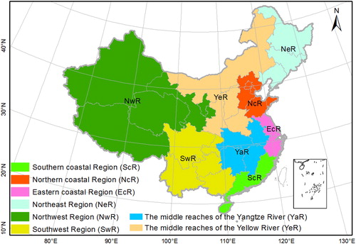
Table 1. The division of eight comprehensive economic zones.

Eight comprehensive economic region	Province
Northeast Region (NeR)	Liaoning, Jilin, Heilongjiang
Northern coastal Region (NcR)	Beijing, Tianjin, Hebei, Shandong
Eastern coastal Region (EcR)	Shanghai, Jiangsu, Zhejiang
Southern coastal Region (ScR)	Fujian, Guangdong, Hainan
The middle reaches of the Yellow River (YeR)	Shanxi, Shaanxi, Henan, Inner Mongolia
The middle reaches of the Yangtze River (YaR)	Hubei, Hunan, Jiangxi, Anhui
Southwest Region (SwR)	Yunnan, Guizhou, Sichuan, Chongqing, Guangxi
Northwest Region (NwR)	Gansu, Qinghai, Ningxia, Xizang, Xinjiang

Note: Hongkong, Macao, and Taiwan haven’t been considered for data unavailability. Abbreviation for each region is in the brackets.

2.2. Data and indicators

The population-weighted average of PM_2.5 concentration ($\mathrm{\mu }\mathrm{g}/{\mathrm{m}}^3$) in Chinese provinces is considered as an ideal indicator for the danger of hazard. On the one hand, the population-weight PM_2.5 data were acquired by dividing the national provinces into a specific grid firstly, then the PM_2.5 concentrations in each grid, based on satellite data, are multiplied by the percentage of inhabitants of the grid in the total population of the province. The population-weighted PM_2.5 is calculated as the population-weighted average of the atmospheric pollution exposure concentrations in all grid regions. That compared to the suburbs or sparsely populated areas, densely populated areas have a higher proportion of the PM_2.5 average in the province, which fully takes into account the difference of low populated, fewer pollution areas and densely populated, highly polluting environments (or vice versa). The weighted population value focuses on the actual impact of inhalable particulate matter on the population, and better reflects the air quality conditions endured by residents in China's provinces.

On the other hand, China began to publish the PM_2.5 data officially since 2012, thus most domestic and foreign scholars use the data of the annual average PM_2.5 concentration ($\mathrm{\mu }\mathrm{g}/{\mathrm{m}}^3$) (2001–2010) supplied by Battelle Memorial Institute and Center for International Earth Science Information Network. And the high macro-analysis value of the data was proved in many studies (Ma and Zhang 2014; Wu et al. 2017). For instance, a table about annual average population-weighted PM_2.5 concentrations with considering the weight of the population in provinces from 2001 to 2010 was estimated by American researchers (Environmental Information Network, 2012). Therefore, the population-weighted average of PM_2.5 concentration (due to the limitation of data sources, the only mainland of China was calculated) was chosen as the hazard index of the disaster-causing factor.

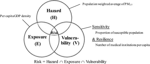
Taking into account the comprehensive situation of regional coverage and social property, resources and infrastructure, the local per capita GDP density (yuan/per capita/km²) is regarded as the exposure index of the disaster-bearing bodies by referring to the existing methods of selecting the exposure index of meteorological disasters (Wang et al. 2014; Ge et al. 2017). Vulnerability index includes two aspects: the sensitivity and the resilience of the hazard-bearing bodies. Considering the main harm of PM_2.5 to human health, especially to the population of the elderly and children (Ye et al. 2016), and to a great extent, the prevention and treatment of hazards are depending on the level of medical equipment in the regions. The vulnerability was considered additionally or specifically in the existing literature about the PM_2.5 pollution assessment (Xie et al. 2014; Wang et al. 2016). Thus, the proportion of the susceptible population (the proportion of the elderly and child population to the total population) and the number of medical institutions per capita were used to represent the sensitivity and resistance of PM_2.5 pollution separately in this paper. Due to the distinctly positive relationship between susceptible population and vulnerability, and the negative correlation between the ability to resist hazards and vulnerability, the vulnerability index (equals to the proportion of the susceptible population divided by the resistance capacity) is constructed to characterize the vulnerability of hazard-bearing bodies. Data about the exposure and vulnerability indexes of the disaster-bearing bodies were derived from the Statistics Yearbook of China (China Statistical Yearbook 2002–2011). And the framework of the PPR assessment by the index system for this article is shown in Figure 2.

Figure 2. The framework of the risk index system for the PPR evaluation.

2.3. Model specification

2.3.1. Concept and properties

The Copula function can combine several variables with inconsistent marginal distributions to form a joint function, and define the domain as [0,1]. It’s basic form as follows (Equation 1(1) $$\begin{array}{c}F\left(x_1,x_2,\dots ,x_N\right)=P\left\{X_1\le x_1,X_2\le x_2,\dots ,X_N\le x_N\right\}\\ =C\left(F_1(x_1),F_2(x_2),\dots ,F_N(x_N)\right)=c\left(u_1,u_2,\dots ,u_N\right)\end{array}$$(1) ), (1) $$\begin{array}{c}F\left(x_1,x_2,\dots ,x_N\right)=P\left\{X_1\le x_1,X_2\le x_2,\dots ,X_N\le x_N\right\}\\ =C\left(F_1(x_1),F_2(x_2),\dots ,F_N(x_N)\right)=c\left(u_1,u_2,\dots ,u_N\right)\end{array}$$(1)

here, N is the dimension of the random variable (number), $x_1,x_2,\dots ,x_N$ is the observed samples. F is the N-dimensional distribution function of the random variable $X_1,X_2,\dots ,X_N,$ C is the joint distribution function, $F_1\left(x_1\right),F_2\left(x_2\right),\dots {,F}_N\left(x_N\right)$ are the marginal distributions of the random variables $X_1,X_2,\dots ,X_N,$ respectively. For simplified expression, let $u_1=F_1\left(x_1\right),$ $u_2=F_2\left(x_2\right),$$\dots ,$$u_N=F_N\left(x_N\right)$ (Joe 1997; Nelsen 2007).

Frank, Gumbel-Hougaard, and Clayton are three classical types of the Archimedean copulas with a single parameter, and the distribution function form and parameter range are displayed in Table 2. The c (u, v, w) represents the copula function, and u, v, and w are the marginal distribution functions of indicators of H, E, and V, respectively. θ is the parameter of the copulas (Kao and Govindaraju 2008).

Table 2. Functions and parameters for three Archimedean copulas.

Type	Basic Copula Function $c(u,v,w)$	Parameter Range
Frank	$-\frac{1}{\theta }\text{ln}\hspace{0.17em}\left[1+\frac{(e^{-\theta u}-1)(e^{-\theta v}-1)(e^{-\theta w}-1)}{{(e^{-\theta }-1)}^2}\right]$	$(-\infty ,\infty )\backslash \left\{0\right\}$
Gumbel-Hougaard	$\text{Exp}\hspace{0.17em}\left\{-{\left[(-\hspace{0.17em}\text{ln}\hspace{0.17em}{u}^{\theta })+(-\hspace{0.17em}\text{ln}\hspace{0.17em}{v}^{\theta })+(-\hspace{0.17em}\text{ln}\hspace{0.17em}{w}^{\theta })\right]}^{\frac{1}{\theta }}\right\}$	$[1,\infty )$
Clayton	$\max \left\{{(u^{-\theta }+v^{-\theta }+w^{-\theta }-2)}^{-1/\theta },0\right\}$	$\left[-1,\infty \right]\backslash \left\{0\right\}$

In this study, the index system of comprehensive PPR is constructed firstly, and the optimal distribution of a single index is determined to prepare for the building of the copula function. And then we try to pick out the optimal Archimedean copula function (Frank, Gumbel-Hougaard, or Clayton) for each region based on the parameter estimation and series of goodness-of-fit tests. The joint distribution function with indicators of H, E, and V (N = 3) will be constructed and analyzed for the comprehensive PPR.

2.3.2. Parameter estimation and goodness-of-fit test

The maximum likelihood estimation (MLE) is the most widely used and relatively flexible method for the parameter estimation of the Copula function. Thus, the MLE is used to estimate the parameters of the marginal distribution of the variables. And the parameters in the copula functions were calculated with the same method. (see Equation 2(2) $$L\left(\theta \right)=\prod _{i=1}^{n}F(x_i;\theta )=\prod _{i=1}^n\frac{\partial F(x_i;\theta )}{\partial x_i}$$(2)  ∼ 4(4) $$\frac{\partial \hspace{0.17em}\text{ln}\hspace{0.17em}\left[L\left(\theta \right)\right]}{\partial \theta }=0$$(4) ). The optimal marginal distribution of each variable is determined by the Anderson - Darling (A-D) goodness-of-fit test. The assessment of the goodness-of-fit of the copula function is realized by constructing the statistic of root mean square error (RMSE), Akaike Information Criterion (AIC), and Bayesian Information Criterion (BIC) (Equation 5(5) $$\mathit{MSE}=\frac{1}{n-m}\sum _{i=1}^n{\left(P{e}_i-P_i\right)}^2$$(5)  ∼ 8(8) $$\mathit{BIC}=n\hspace{0.17em}\text{ln}\hspace{0.17em}(\mathit{MSE})+m\hspace{0.17em}\text{ln}\hspace{0.17em}(n)$$(8) ), and which can determine the optimum copula function (Karmakar and Simonovic 2009; Zhang et al. 2017). (2) $$L\left(\theta \right)=\prod _{i=1}^{n}F(x_i;\theta )=\prod _{i=1}^n\frac{\partial F(x_i;\theta )}{\partial x_i}$$(2) (3) $$\text{ln}\hspace{0.17em}\left[L(\theta )\right]=\sum _{i=1}^n\hspace{0.17em}\text{ln}\hspace{0.17em}\left[F(x_i;\theta )\right]$$(3) (4) $$\frac{\partial \hspace{0.17em}\text{ln}\hspace{0.17em}\left[L\left(\theta \right)\right]}{\partial \theta }=0$$(4) (5) $$\mathit{MSE}=\frac{1}{n-m}\sum _{i=1}^n{\left(P{e}_i-P_i\right)}^2$$(5) (6) $$\mathit{RMSE}=\sqrt{\mathit{MSE}}$$(6) (7) $$\mathit{AIC}=n\hspace{0.17em}\text{ln}\hspace{0.17em}(\mathit{MSE})+2m$$(7) (8) $$\mathit{BIC}=n\hspace{0.17em}\text{ln}\hspace{0.17em}(\mathit{MSE})+m\hspace{0.17em}\text{ln}\hspace{0.17em}(n)$$(8)

Where, L(θ) is the likelihood function. F(x_i, θ) is the marginal distribution function, θ is the parameter to be estimated. RMSE represents the root mean square error. The smaller the value of RMSE, AIC, and BIC, the better the fitting of the model. m is the number of parameters in the copula function, and which equals to 1 in this paper. n is the sample size. And this study considered 31 provinces with 10-year data (2001 ∼ 2010). The sample size for the whole mainland is 310 (n = 310). Similarly, for the ECE regions, the sample size is the number of provinces in each region multiplied by 10 (n is 30, 40 or 50, respectively). Both of them are satisfied with the requirement of the probability distribution fitting.

2.3.3. Conditional distribution function

In the conditional joint distribution function of the three-dimensional variable, when the variable $X_2=x_2$ and $X_3=x_3,$ the basic form of the conditional distribution function of the variable $X_1$ is Equation 9(9) $$c(u|v,w)=F(X_1\le x_1|X_2=x_2,X_3=x_3)=\frac{\frac{{\partial }^{2}c(u,v,w)}{\partial v\partial w}}{\frac{{\partial }^{2}c(v,w)}{\partial v\partial w}}$$(9) (Zhang and Singh 2017b): (9) $$c(u|v,w)=F(X_1\le x_1|X_2=x_2,X_3=x_3)=\frac{\frac{{\partial }^{2}c(u,v,w)}{\partial v\partial w}}{\frac{{\partial }^{2}c(v,w)}{\partial v\partial w}}$$(9) where u, v, w are the marginal distribution functions of the random variables $X_1,X_2,X_3,$ respectively. Based on Equation 9(9) $$c(u|v,w)=F(X_1\le x_1|X_2=x_2,X_3=x_3)=\frac{\frac{{\partial }^{2}c(u,v,w)}{\partial v\partial w}}{\frac{{\partial }^{2}c(v,w)}{\partial v\partial w}}$$(9) , we can calculate the probability (P) of $X_1>x_1$ by the following function (Equation 10(10) $$P(X_1>x_1|X_2=x_2,X_3=x_3)=1-F(X_1\le x_1|X_2=x_2,X_3=x_3)$$(10) ) when $X_2=x_2$ and $X_3=x_3.$ (10) $$P(X_1>x_1|X_2=x_2,X_3=x_3)=1-F(X_1\le x_1|X_2=x_2,X_3=x_3)$$(10)

In conditional probability analysis, the risk probability of the hazard indicator PM_2.5 exceeding the given threshold value will be calculated under given exposure and vulnerability condition ($X_2=x_2$ and $X_3=x_3$).

3. Result analysis

3.1. The marginal distributions of the risk factors

The risk factors H, E, and V of the PM_2.5 pollution are all continuous random variables, and the marginal distribution of the univariate was obtained based on the parameter estimation. The considered marginal distribution for the single variable includes Beta, Exponential, Extreme value, Gamma, Logistic, Log-logistic, Lognormal, Normal, Generalized extreme value, and Weibull distribution. The optimal marginal distribution was established by the A-D test (Table 3). In Table 3, Weibull and Gamma are the main types of the univariates, especially for H and V, with Lognormal and Generalized extreme value distribution followed. The E indicator takes a high proportion of Lognormal distribution. The only E in YeR and ScR is Exponential distribution.

Table 3. Marginal distribution of each variable (H, E, and V) for regions.

Region	Variable	Marginal distribution	Region	Variable	Marginal distribution
NeR	H	Weibull	YeR	H	Weibull
	E	Lognormal		E	Exponential
	V	Weibull		V	Gamma
NcR	H	Gamma	YaR	H	Weibull
	E	Gamma		E	Lognormal
	V	Weibull		V	Weibull
EcR	H	Gamma	SwR	H	Weibull
	E	Generalized Extreme Value		E	Lognormal
	V	Gamma		V	Gamma
ScR	H	Weibull	NwR	H	Lognormal
	E	Exponential		E	Generalized Extreme Value
	V	Generalized Extreme Value		V	Weibull
China	H	Generalized Extreme Value
	E	Lognormal
	V	Gamma

3.2. Parameter estimation and selection of copula function

The MLE method is used to estimate the parameters of three-dimensional Archimedean copula (Equation 2(2) $$L\left(\theta \right)=\prod _{i=1}^{n}F(x_i;\theta )=\prod _{i=1}^n\frac{\partial F(x_i;\theta )}{\partial x_i}$$(2)  ∼ 4(4) $$\frac{\partial \hspace{0.17em}\text{ln}\hspace{0.17em}\left[L\left(\theta \right)\right]}{\partial \theta }=0$$(4) ). The optimal copula function (Frank, Gumbel-Houggard, or Clayton) is selected by the statistical RMSE, AIC, BIC (Equation 5(5) $$\mathit{MSE}=\frac{1}{n-m}\sum _{i=1}^n{\left(P{e}_i-P_i\right)}^2$$(5)  ∼ 8(8) $$\mathit{BIC}=n\hspace{0.17em}\text{ln}\hspace{0.17em}(\mathit{MSE})+m\hspace{0.17em}\text{ln}\hspace{0.17em}(n)$$(8) ), and the correlation coefficient (R²) of the empirical probability (P_ei) and theoretical probability (P_i) (Li et al. 2013). The results are shown in Table 4.

Table 4. Parameter estimation and the optimal copula function selection.

Region	Type	θ	RMSE	AIC	BIC	R^2 (Pei -Pi)
NeR	Frank	0.8854	0.0036	−166	−165	0.9344
	Gumbel	1.0789	0.0036	−166	−165	0.9367
	Clayton	0.2556	0.0032	−170	−168	0.9361
NcR	Frank	—	—	—	—	—
	Gumbel	1.011	0.0025	−238	−236	0.8132
	Clayton	—	—	—	—	—
EcR	Frank	0.9755	0.0085	−141	−140	0.8633
	Gumbel	1.0840	0.0092	−138	−137	0.8587
	Clayton	0.4585	0.0066	−148	−147	0.8671
ScR	Frank	—	—	—	—	—
	Gumbel	1.015	0.0028	−174	−172	0.7280
	Clayton	—	—	—	—	—
YeR	Frank	3.9873	0.0021	−244	−242	0.9857
	Gumbel	1.5835	0.0027	−234	−232	0.9854
	Clayton	0.8876	0.0022	−242	−240	0.9843
YaR	Frank	1.6773	0.0020	−246	−244	0.9814
	Gumbel	1.1756	0.0025	−237	−235	0.9818
	Clayton	0.5660	0.0015	−258	−256	0.9814
SwR	Frank	0.3064	0.0030	−288	−286	0.9516
	Gumbel	1.0226	0.0032	−285	−284	0.9508
	Clayton	0.1069	0.0028	−292	−290	0.9520
NwR	Frank	0.8573	0.0028	−291	−289	0.9835
	Gumbel	1.0916	0.0030	−288	−286	0.9833
	Clayton	0.1863	0.0028	−291	−290	0.9836
China	Frank	1.9531	5.77 × 10^−4	−2.31 × 10^−3	−2.31 × 10^−3	0.9941
	Gumbel	1.2003	6.29 × 10^−4	−2.13 × 10^−3	−2.12 × 10^−3	0.9911
	Clayton	0.4217	10.00 × 10^−4	−2.28 × 10^−3	−2.28 × 10^−3	0.9931

Note: (1) ‘Gumbel’ represents ‘Gumbel-Hougaard’ Copula for space-saving. (2) ‘—’ is the estimated parameter that out of defined range and not suitable for the copula construction. (3) R² are all passed the significance test (α = 0.01). (4) Bold contents are the optimal copula functions and their related fitting optimization index.

In Table 4, in NcR and ScR, only the Gumbel copula satisfied the threshold requirements of the parameter. The R² is relatively low compared with that of the other regions (NcR: 0.8132 and ScR: 0.7280, respectively), but all of them passed the 0.01 significant test. Although the R² of the Gumbel copula in NeR and YaR is the highest (higher than that of the frank and Clayton functions), the numerical difference is tiny. Thus the optimal copula in this study is ultimately determined by the RMSE, AIC, and BIC, and the R² is an auxiliary reference. The copula type with bold font in Table 4 is the optimal copula function for each region of the final selection.

3.3. Risk analysis of the PM_2.5 pollution

3.3.1. Comprehensive risk analysis

According to the selected optimal Archimedean Copula function, the joint probability of a three-dimensional variable of PM_2.5 pollution was calculated, and the three-dimensional joint cumulative probability risk for each region was plotted (Figure 3).

Figure 3. The cumulative probability of the PPR for all regions.

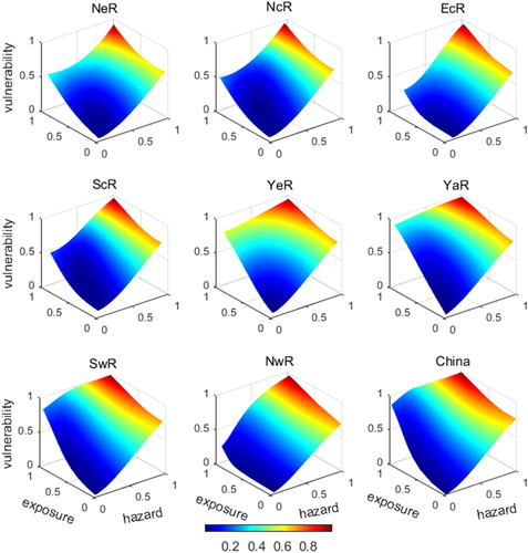
As shown in Figure 3, the result of the multivariable copula is a representation of the probability of the comprehensive PPR. Taking the NcR as an example, the dot (0.53, 0.75, 0.44, 0.20) indicates that the cumulative probabilities of the E and V are 0.75 and 0.44 respectively when H is 0.53, the risk of the corresponding Clayton copula probability value is 0.20. The numerical difference of H-E-V reflects the change of the PPR under different probability combinations. The copula with multi-factors contains more information than that of a single variable and makes the links among risk factors prominently, and which is deficient and must be explored in the existing risk analysis.

Through a comparative analysis of Figure 3, the joint cumulative probability in NeR, NcR, EcR, ScR and NwR shows a significant ‘concave’ feature, which indicates that the risk is very low (usually less than 0.2) when the risk factor (H, E, V) is small (less than 0.5). A similar trend of the cumulative probability risk was found in YeR, YaR, SeR, and the whole mainland, respectively. That is, the probability of the risk is still small (less than 0.5) when the disaster factors (H and E) take a smaller value (less than 0.5), and the vulnerability index takes a larger value (more than 0.5). When the risk factors (H and E) take the larger value (more than 0.8) and the vulnerability index does not change significantly (still more than 0.5), the risk is very high (closes to 1).

The cumulative probability of the PPR is monotone increasing with each variable of the indicators, and which is up to the objective fact of the cumulative probability distribution, that is, H ∼ E∼V is close to (1, 1, 1) when the copula value also approaches 1 (Figure 3). Because of the desynchrony of the joint variables and the fitting errors of the optimal Archimedean copula, the copula value in the vicinity of H ∼ E∼V (0.5, 1, 1) in SwR and the whole mainland of China is close to 1, and which belongs to the phenomenon that the copula cumulative distribution value is abnormally high. But the small error has little influence on the objective law that the cumulative distribution value of copula is monotone increasing with the variable. And the selected copula function is the optimal three-variable joint distribution through the test of RMSE, AIC, BIC, and R². Thus the calculated results of joint cumulative probability can reflect the comprehensive risk of each region.

3.3.2. Conditional probability analysis

In China, the PM_2.5 concentration thresholds were added in the newly revised National Ambient Air Quality Standard (NAAQS), and the Daily Average Concentration Limit Level I and II are 35 $\mathrm{\mu }\mathrm{g}/{\mathrm{m}}^3$ and 75$\text{µg}/{\mathrm{m}}^3$ respectively, but they are just the international minimum standard. According to the rule of Environmental Protection Agency (EPA) of the USA, the air quality is good when the daily average concentration is lower than 15 $\mathrm{\mu }\mathrm{g}/{\mathrm{m}}^3,$ and which is no harm to health; while that of the concentration is higher than 65 $\mathrm{\mu }\mathrm{g}/{\mathrm{m}}^3$ indicates that air quality is harmful to life (Zhou and Ru 2012; Zhang and Cao 2015). Hereby the risk changes of the population-weighted average PM_2.5 concentration thresholds of 15 $\mathrm{\mu }\mathrm{g}/{\mathrm{m}}^3$ (good air quality) and 35$\text{μg}/{\mathrm{m}}^3$ (the daily average concentration limit) were considered by combing the two sides in this study. The risk probabilities of the H more than 15 $\mathrm{\mu }\mathrm{g}/{\mathrm{m}}^3$ and 35$\text{μg}/{\mathrm{m}}^3$ under different combinations of the E and V are calculated according to the Equation 9 ∼ 10. The probability of the H exceeding the pre-setting thresholds could be searched under any combinations of the E and V based on Figures 4 and 5.

Figure 4. Contours of the conditional probability that the hazard index exceeding 15 $\mathrm{\mu }\mathrm{g}/.$${\mathrm{m}}^3$

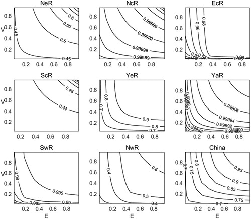
Figure 5. Contours of the conditional probability that the hazard index exceeding 35 $\mathrm{\mu }\mathrm{g}/.$${\mathrm{m}}^3$

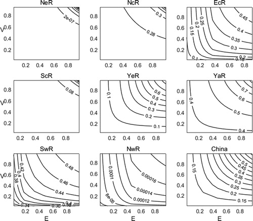
By comparing and analyzing the conditional probability graphs of different regions, firstly, the probability that more than 15 $\mathrm{\mu }\mathrm{g}/{\mathrm{m}}^3$ (Figure 4), it is found that the exceedance probability of the NcR, EcR, YaR, and SwR are all close to 1 regardless of the combinations of the E and V, and which indicates that the PPR in these areas is the highest (>0.96). It is difficult to maintain good air quality. And the following is that the risk in YeR is the higher (0.61 ∼ 0.99), and the probability risk value in NwR, NeR, and ScR that fluctuates between 0.40 ∼ 0.65, the PPR is lower than that of other regions. The value of the whole area is 0.69 ∼ 0.98, and the probability approximates to the value in YeR.

Secondly, the probability that more than 35 $\mathrm{\mu }\mathrm{g}/{\mathrm{m}}^3$ (Figure 5), the results show that the risk in most regions is lower than 0.5. Among them, the exceeding probability is the lowest level (closes to 0) in NeR (≤ 1.05 × 10⁻⁶) and NwR (0.52 × 10⁻⁴ ∼1.90 × 10⁻⁴), which means that the PM_2.5 pollution is almost impossible in the two regions. And the risk is also low in ScR (0.07 ∼ 0.21), NcR (0.27 ∼ 0.40), EcR (0.06 ∼ 0.49), as well as SwR (0.30 ∼ 0.50). The risk in YeR (0.04 ∼ 0.81) and YaR (0.34 ∼ 0.95) is relatively high, and the value of the whole country is 0.11 ∼ 0.67, which belongs to the medium level. According to the probability average, only the conditional probability in YaR is more than 0.5 (0.58), thus the YaR belongs to the highest level.

In addition, it can be seen from Figures 4 and 5 that the contours are densely distributed of the corresponding Z-axis (vulnerability index) in some regions (EcR, SwR, and NwR). They indicate the smaller changes of the vulnerability index will lead to greater variations, and which means V is more sensitive than E to the risk in these zones.

To display the PPR of the ECE zones in China more clearly and intuitively, the average of the conditional probability of each region is arranged in order from low to high, and the relative risk of each region can be seen from the spatial graphs (Figure 6).

Figure 6. The relative risk under different thresholds for the ECE regions in China.

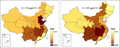
In Figure 6, the probability of exceeding good air quality standards (15 $\mathrm{\mu }\mathrm{g}/{\mathrm{m}}^3$) in NcR (Beijing, Tianjin, Hebei, and Shandong) is the highest, and the relative risk in ScR, NeR, and NwR is lower which can keep air quality good. Meanwhile, exceeding the probability of the daily average concentration limit (35$\text{μg}/{\mathrm{m}}^3$) in NeR, NwR, and ScR is also relatively small, while the highest risk is in YaR (Hubei, Hunan, Jiangxi, Anhui). Overall, the low PPR is mainly distributed in NeR, ScR, and NwR. The high-risk zone will change with the thresholds in YaR or NcR.

4. Discussion

The optimum copula type was selected separately in each comprehensive economic zones in this paper. The correlation coefficients of the empirical probability and the theoretical probability in most regions are high values (greater than 0.85) except that in NcR and ScR. It indicates that the model has good explanatory ability and can reflect the degree of regional risk objectively.

To better understand the physical mechanism of the impact of these three indicators on risk, the spatial distribution of the mean values of the three risk impact indicators in the ECE regions, as illustrated in Figure 7. Three impact indicators (H, E, and V) in NeR are the lowest values (Figure 7 and Table 5), followed by that in NwR. While the highest values are in different areas, the highest value of H E and V appeared in NcR, EcR, and YaR, respectively. Thus, it is hard to judge the risk level of each region by a single factor through linear sorting directly and objectively.

Figure 7. Average of each economic region of the three indexes (H, E & V).

Table 5. Rank for the ECE regions of the risk factors and the relative risk under different thresholds.

Indicator		Rank for the eight regions from low to high（Level 1 ∼ 8）
		Low $\to$ Medium $\to$ High
Level		1	2	3	4	5	6	7	8
Hazard Index		NeR	NwR	ScR	YeR	EcR	SwR	YaR	NcR
Exposure Index		NeR	NwR	YeR	YaR	SwR	ScR	NcR	EcR
Vulnerability Index		NeR	NwR	NcR	YeR	ScR	EcR	SwR	YaR
Relative risk	> 15$\mathbf{\mu }\mathbf{g}/{\mathbf{m}}^3$	ScR	NeR	NwR	YeR	EcR	SwR	YaR	NcR
	> 35$\mathbf{\mu }\mathbf{g}/{\mathbf{m}}^3$	NeR	NwR	ScR	NcR	EcR	YeR	SwR	YaR

However, combined the spatial distribution map of the single-factor index (Figure 7) with the relative risk ranking under different thresholds (Figure 6 and Table 5), some rules were illustrated that reflected the physical mechanism of these factors on the relative PPR to some extent. For instance, in NeR, where the average of each of the three indicators is the lowest (Level 1), the risk probabilities exceeding 15 $\mathrm{\mu }\mathrm{g}/{\mathrm{m}}^3$ and 35 $\mathrm{\mu }\mathrm{g}/{\mathrm{m}}^3$ are both the lowest levels (Level 2 and 1, respectively). In NcR, although H and E are relatively high (Level 8 and Level 7, respectively), their vulnerability index values are relatively low (Level 3), and the risk probability exceeding the lower threshold (15 $\mathrm{\mu }\mathrm{g}/{\mathrm{m}}^3$) is the highest (Level 8). But the risk exceeding the higher threshold (35 $\mathrm{\mu }\mathrm{g}/{\mathrm{m}}^3$) is moderate (Level 4). In EcR, since E is the only at the highest level (Level 8) and the other two indicators (H and V) are at the medium level (Level 5 and 6, respectively), the relative risk is at the medium level (Level 5). Since the areas with the high values of H and V, and the low value of E, the risk of exceeding probability is also high, such as YaR and SwR.

To sum up, the H and V have a more direct impact on the PPR than the E. Therefore, reducing the pollutant emission (especially the PM_2.5) and improving the response capacity is essential to the regional risk control and management. Although the exposure of disaster-bearing bodies can reflect economic power to a certain extent, the results of this study do not show the E has a direct impact on the PPR. While it has been proved that there is an upward u-shaped relationship between them (Wu et al. 2017). Thus, at the same time of promoting regional economic development, avoiding the exposure of disaster-bearing bodies to disaster-causing factors reasonably and effectively and reducing the adverse effects of economic development to the atmospheric environment couldn’t be ignored. Also, to evaluate the PPR, the overall impact of these three aspects should be taken into account spontaneously to draw an objective conclusion.

5. Conclusion

The PPR evaluation is not easy for the complex impactors and interaction mechanism. This study tried to conform to reality, to quantify the PPR from the ECE zones to the whole mainland in China in the perspective of the modern hazard risk assessment. Based on the three-dimensional copula method, we consider the H, E, and V simultaneously to ensure the objectivity and the accuracy of the risk assessment.

The analysis results show that: (i) The comprehensive PPR is monotone increasing with the H, E and V, and which can be obtained from the joint cumulative probability figure. (ii) According to the conditional probability analysis, it is hard to ensure good air quality (less than 15 $\mu g/m^3$) in NcR, EcR, YaR, and SwR. It is consistent with the actual regional distribution of air pollution in previous studies, the air pollution of these areas is more serious, and the PPR is high (Tao et al. 2014; Wang et al. 2014; Cheng et al. 2017; Wu et al. 2017); the risk in all regions that exceeding the daily average concentration limit (more than 35 $\mu g/m^3$) is not high (the average lower than 0.5) except in YaR; the lowest risk appears in NeR, NwR, and ScR under both thresholds. (iii) Although the single indicator can reflect the physical mechanism of the risk to some extent, the relationship between the impact factors and the risk is always nonlinear. The H and V have a more direct impact on the PPR than the E, and the comprehensive assessment with all of the three aspect indicators is vital.

At the methodological level, the application of the copula function in the multi-dimensional elements joint risk can widen the research of the multiple factors joint assessment of disaster risk. The high correlation between the variables will reduce the precision of the model to some extent. The correlation coefficients of the theoretical distributions and empirical distributions in NcR and ScR in the study were relatively low (0.81 and 0.73, although they passed the significant tests that show the model is feasible), and the main reason is that the correlation between the H and E is higher (R² is -0.64 and -0.83, respectively). In future research, we will try to explore other types of copula functions to improve the accuracy and reliability of the model. The selection of other related indexes for the risk assessment and the extension of available data of the time series and the analysis of the dynamic change of risk in space could be further tried and expanded.

Additional information

Funding

This work was subsidized by the National Natural Science Foundation of China (Grant No. 41501555 & 91546117), the major project of National Social and Scientific Fund Program (Grant No. 16ZDA047), the open project of Institute of Climate Change and public policy (Grant No. 14QHA009), and the sponsorship of Jiangsu Oversea Visiting Scholar Program for University Prominent Young & Middle-aged Teachers and Presidents.

References

- Atkinson RW, Kang S, Anderson HR, Mills IC, Walton HA. 2014. Epidemiological time series studies of PM2.5 and daily mortality and hospital admissions: a systematic review and meta-analysis. Thorax. 69(7):660–665.
- Carrao H, Naumann G, Barbosa P. 2016. Mapping global patterns of drought risk: An empirical framework based on sub-national estimates of hazard, exposure and vulnerability. Global Environ Change. 39:108–124.
- Chen P, Bi X, Zhang J, Wu J, Feng Y. 2015. Assessment of heavy metal pollution characteristics and human health risk of exposure to ambient PM2.5 in Tianjin, China. Particuology. 20:104–109.
- Chen Z, Chen D, Xie X, Cai J, Zhuang Y, Cheng N, He B, Gao B. 2019. Spatial self-aggregation effects and national division of city-level PM2.5 concentrations in China based on spatio-temporal clustering. J Clean Prod. 207:875–881.
- Chen Z, Xie X, Cai J, Chen D, Gao B, He B, Cheng N, Xu B. 2018. Understanding meteorological influences on PM2.5 concentrations across China: a temporal and spatial perspective. Atmos Chem Phys. 18(8):5343–5358.
- Cheng Z, Li L, Liu J. 2017. Identifying the spatial effects and driving factors of urban PM2.5 pollution in China. Ecol Indic. 82:61–75.
- Environmental Information Network. 2012. A panorama of air pollution in China seen from space. [accessed 2019 March 5]. http://www.12369.com.cn/news/detail?id=1403.
- Fu G, Butler D. 2014. Copula-based frequency analysis of overflow and flooding in urban drainage systems. J Hydrol. 510:49–58.
- Gao M, Guttikunda SK, Carmichael GR, Wang Y, Liu Z, Stanier CO, Saide PE, Yu M. 2015. Health impacts and economic losses assessment of the 2013 severe haze event in Beijing area. Sci Total Environ. 511:553–561.
- García-Santiago X, Gallego-Fernández N, Muniategui-Lorenzo S, Piñeiro-Iglesias M, López-Mahía P, Franco-Uría A. 2017. Integrative health risk assessment of air pollution in the northwest of Spain. Environ Sci Pollut Res. 24(4):3412–3422.
- Ge Y, Zhang H, Dou W, Chen W, Liu N, Wang Y, Shi Y, Rao W. 2017. Mapping social vulnerability to air pollution: a case study of the Yangtze River Delta region, China. Sustainability. 9(1):109.
- He J, Gong S, Yu Y, Yu L, Wu L, Mao H, Song C, Zhao S, Liu H, Li X, et al. 2017. Air pollution characteristics and their relation to meteorological conditions during 2014–2015 in major Chinese cities. Environ Pollut. 223:484–496.
- Huang R, Zhang Y, Bozzetti C, Ho KF, Cao JJ, Han Y, Daellenbach KR, Slowik JG, Platt SM, Canonaco F, et al. 2014. High secondary aerosol contribution to particulate pollution during haze events in China. Nature. 514(7521):218.
- Jiang P, Yang J, Huang C, Liu H. 2018. The contribution of socioeconomic factors to PM2.5 pollution in urban China. Environ Pollut. 233:977–985.
- Joe H. 1997. Multivariate models and multivariate dependence concepts. New York: CRC Press.
- Kao SC, Govindaraju RS. 2008. Trivariate statistical analysis of extreme rainfall events via the Plackett family of copulas. Water Resour Res. 44(2):1–19.
- Karmakar S, Simonovic SP. 2009. Bivariate flood frequency analysis. Part 2: a copula‐based approach with mixed marginal distributions. J Flood Risk Manage. 2(1):32–44.
- Koks EE, Jongman B, Husby TG, Botzen WJW. 2015. Combining hazard, exposure and social vulnerability to provide lessons for flood risk management. Environ Sci Policy. 47:42–52.
- Lang J, Cheng S, Li J, Chen D, Zhou Y, Wei X, Han L, Wang H. 2013. A monitoring and modeling study to investigate regional transport and characteristics of PM2.5 pollution. Aerosol Air Qual Res. 13(3):943–956.
- Lavell A, Oppenheimer M, Diop C, Hess J, Lempert R, Li J, Cardona OD. 2012. Climate change: new dimensions in disaster risk, exposure, vulnerability, and resilience In: Field C B, Barros V, Stocker T F, Qin D, Dokken D J, Ebi K L, Mastrandrea M D, Mach K J, Plattner G-K, Allen S K, Tignor M, and Midgley P M, editors. Managing the risks of extreme events and disasters to advance climate change adaptation: special report of the intergovernmental panel on climate change. Cambridge and New York: Cambridge University Press. p: 25–64.
- Li N, Liu X, Xie W, Wu J, Zhang P. 2013. The return period analysis of natural disasters with statistical modeling of bivariate joint probability distribution. Risk Anal. 33(1):134–145.
- Lin G, Fu J, Jiang D, Hu W, Dong D, Huang Y, Zhao M. 2013. Spatio-temporal variation of PM2.5 concentrations and their relationship with geographic and socioeconomic factors in China. Int J Environ Res Public Health. 11(1):173–186.
- Liu X, Li N, Yuan S, Xu N, Shi W, Chen W. 2015. The joint return period analysis of natural disasters based on monitoring and statistical modeling of multidimensional hazard factors. Sci Total Environ. 538:724–732.
- Lu F, Xu D, Cheng Y, Dong S, Guo C, Jiang X, Zheng X. 2015. Systematic review and meta-analysis of the adverse health effects of ambient PM2.5 and PM10 pollution in the Chinese population. Environ Res. 136:196–204.
- Ma LM, Zhang X. 2014. The spatial effect of haze pollution in China and the impact from economic change and energy structure. China Ind Econ. 4:19–31.
- Mach K, Mastrandrea M. 2014. Climate change 2014: impacts, adaptation, and vulnerability. Vol. 1. Field CB, Barros VR, editors. The Fifth Assessment Report (AR5) of the Intergovernmental Panel on Climate Change (IPCC) — Climate Change 2013/2014. Cambridge: Cambridge University Press.p:1371–1438.
- Milla dos Santos AP, Passuello A, Schuhmacher M, Nadal M, Domingo JL, Martinez CA, Segura-Munoz SI, Takayanagui AMM. 2014. A support tool for air pollution health risk management in emerging countries: a case in Brazil. Hum Ecol Risk Assess: Int J. 20(5):1406–1424.
- Ming X, Xu W, Li Y, Du J, Liu B, Shi P. 2015. Quantitative multi-hazard risk assessment with vulnerability surface and hazard joint return period. Stochastic Environ Res Risk Assess. 29(1):35–44.
- Nelsen RB. 2007. An introduction to copulas. Portland, USA: Springer Science & Business Media.
- Pui DYH, Chen SC, Zuo Z. 2014. PM2.5 in China: measurements, sources, visibility and health effects, and mitigation. Particuology. 13:1–26.
- Pun VC, Kazemiparkouhi F, Manjourides J, Suh HH. 2017. Long-term PM2.5 exposure and respiratory, cancer, and cardiovascular mortality in older US adults. Am J Epidemiol. 186(8):961–969.
- Rodriguez JC. 2007. Measuring financial contagion: a copula approach. J Empirical Finance. 14(3):401–423.
- Tao J, Gao J, Zhang L, Zhang R, Che H, Zhang Z, Lin Z, Jing J, Cao J, Hsu SC. 2014. PM2.5 pollution in a megacity of southwest China: source apportionment and implication. Atmos Chem Phys. 14(16):8679–8699.
- Wang B, Chen Z. 2010. A GIS-based fuzzy aggregation modeling approach for air pollution risk assessment. In 2010 Seventh International Conference on Fuzzy Systems and Knowledge Discovery. Yantai, China. Vol. 2: IEEE. p. 957–961.
- Wang G, Gu S, Chen J, Wu X, Yu J. 2016. Assessment of health and economic effects by PM2.5 pollution in Beijing: a combined exposure-response and computable general equilibrium analysis. Environ Technol. 37(24):3131–3138.
- Wang S, Zhou C, Wang Z, Feng K, Hubacek K. 2017. The characteristics and drivers of fine particulate matter (PM2.5) distribution in China. J Clean Prod. 142:1800–1809.
- Wang Y, Gao C, Wang A, Wang Y, Zhang F, Zhai J, Li X, Su B. 2014. Temporal and spatial variation of exposure and vulnerability of flood disaster in China. Adv Clim Change Res. 10:391–398.
- Wang Y, Ying Q, Hu J, Zhang H. 2014. Spatial and temporal variations of six criteria air pollutants in 31 provincial capital cities in China during 2013–2014. Environ Int. 73:413–422.
- Wu J, Zheng H, Zhe F, Xie W, Song J. 2018. Study on the relationship between urbanization and fine particulate matter (PM2.5) concentration and its implication in China. J Clean Prod. 182:872–882.
- Wu X, Chen Y, Guo J, Wang G, Gong Y. 2017. Spatial concentration, impact factors and prevention-control measures of PM2.5 pollution in China. Nat Hazards. 86(1):393–410.
- Xie Y, Chen J, Li W. 2014. An assessment of PM2.5 related health risk and impaired values of Beijing residents in a consecutive high-level exposure during heavy haze days. Environ Sci. 35(1):1–8.
- Yang D, Ye C, Wang X, Lu D, Xu J, Yang H. 2018. Global distribution and evolvement of urbanization and PM2.5 (1998–2015). Atmos Environ. 182:171–178.
- Yang K, Yang Y, Zhu Y, Li C, Meng C. 2016. Social and economic drivers of PM2.5 and their spatial relationship in China. Geog Res. 35:1051–1060.
- Ye Q, Fu JF, Mao JH, Shang SQ. 2016. Haze is a risk factor contributing to the rapid spread of respiratory syncytial virus in children. Environ Sci Pollut Res Int. 23(20):20178–20185.
- Zhang L, Singh VP. 2007a. Bivariate rainfall frequency distributions using Archimedean copulas. J Hydrol. 332(1–2):93–109.
- Zhang L, Singh VP. 2007b. Gumbel–Hougaard copula for trivariate rainfall frequency analysis. J Hydrol Eng. 12(4):409–419.
- Zhang Q, Crooks R. 2012. Toward an environmentally sustainable future: country environmental analysis of the People's Republic of China. Mandaluyong City, Philippines: Asian Development Bank.
- Zhang Y, Cao F. 2015. Fine particulate matter (PM2.5) in china at a city level. Sci Rep. 5(1):14884.
- Zhang Y, Wang K, Liu X, Zhang S, Zhou J, Wang C. 2017. The three-dimensional joint distributions of rainstorm factors based on copula function: a case in Kuandian county, Liaoning province. Sci Geog Sin. 37:603–610.
- Zhang YL, Cao F. 2015. Fine particulate matter (PM 2.5) in China at a city level. Sci Rep. 5:14884.
- Zheng X, Xu X, Yekeen TA, Zhang Y, Chen A, Kim SS, Dietrich KN, Ho S-M, Lee S-A, Reponen T, et al. 2016. Ambient air heavy metals in PM2.5 and potential human health risk assessment in an informal electronic-waste recycling site of China. Aerosol Air Qual Res. 16(2):388–397.
- Zhou L, Wu X, Ji Z, Gao G. 2017. Characteristic analysis of rainstorm-induced catastrophe and the countermeasures of flood hazard mitigation about Shenzhen city. Geomat Nat Hazards Risk. 8(2):1886–1897.
- Zhou T, Ru X. 2012. Research on the cause and treatment of haze in Beijing. J North China Electr Power Univ (Social Sciences). 2:12–16.
- Zhu L, Gong X, Shen J, Liu L, Liu JF, Liu JL, Xu Z. 2019. Application of computational aerodynamics on the risk prediction of PM2.5 in congenital tracheal stenosis. In: Lhotska L, Sukupova L, Lacković I, Ibbott G, editors. World congress on medical physics and biomedical engineering 2018. IFMBE Proceedings. Singapore: Springer. p: 807–811.