Geospatial analysis of September, 2019 floods in the lower gangetic plains of Bihar using multi-temporal satellites and river gauge data

Abstract

During late September, 2019 Bihar was struggling with severe flooding problem, which otherwise is marked as a period of flood recession due to withdrawal of south-east monsoons. The present study assess the flood situation using Sentinel-1 SAR images and complements the understanding about the flood event using long term (2000-18) multi-temporal space based flood sensitive proxy indicators like precipitation (GPM), soil moisture (AMSR-2), vegetation condition (MODIS) together with ground based river gauge (CWC) data. The study reveals that in 2019 during the 39^th week of the year (late September) the central and eastern parts of Bihar witnessed heavy precipitation (176 percent higher than average), leading to enhanced soil moisture build up (19 percent higher than average) and consequently triggering severe flooding. River Ganga was observed to be flowing above danger level for almost two weeks. Due to the prolonged submergence by floodwaters a significant drop was observed in the NDVI and EVI values of about 13.7 and 11.1 percent respectively from the normal. About 8.36 lakh ha area was observed to be inundated, impacting about 9.26 million population. Patna followed by Bhagalpur were the two worst affected districts with almost 30% and 36% of districts geographical area being flooded.

Keywords:

• Bihar
• disaster
• floods
• Sentinel-1
• satellite

1. Introduction

The ‘extreme’ weather events are becoming the new ‘normal’, and during every monsoon season previous flood records are being breached recurrently in Indian sub-continent (Prasad et al. 2005; Guhathakurta et al. 2011; Jena et al. 2014; Mishra et al. 2018; Ray et al. 2019). The recent past flood events across the Indian landscape, like the Mumbai floods (2005), Kosi floods (2008), Leh flash floods (2011), Kedarnath flash floods (2013), Jhelum floods (2014), Chennai floods (2015), Brahmaputra floods (2012), Kerala floods (2018) and the Ganga floods of Bihar (2019) are examples of increasing severity of hydrological disasters. The river gauge data shows that the rivers are breaching their high flood levels more often in the last one decade than ever due to increasing extreme events (Bhatt and Rao 2016). As the severity and frequency of extreme events is increasing, there is an urgent need for understanding the disaster risk in all its dimensions as outlined under the first priority of Sendai Framework for Disaster Risk Reduction (SFDRR). For assessing the risk due to flood events and formulating any flood risk management strategies, information about the flood hazard in spatial and temporal scales is an important input.

The mapping and monitoring of dynamic events like flood hazard, which have a regional footprint has been greatly benefitted from the synthetic aperture radar (SAR) systems. The SAR systems with longer wavelengths are able to penetrate the cloud cover and therefore have emerged as one of the potential source for mapping and monitoring the flood hazards (Prasad et al. 2006; Singh et al. 2009; Bhatt et al. 2017; Borah et al. 2018; Mishra et al. 2018; Vishnu et al. 2019). Due to the high cost of SAR data, requirement of separate processing software’s and limitation of processing systems, the flood studies were limited to smaller extents despite the potential SAR data offered. However, in recent times the continuous streaming of free microwave radar data from Sentinel-1 constellation (Sentinel-1A and -1B) from European Space Agency (ESA) under the auspices of the Copernicus Earth observation program has significantly aided the flood hazard research and flood response activities (Berezowski et al. 2020). The potential of Sentinel SAR data potential has been further enhanced with the emergence of freely accessible web based cloud computing services like the Google Earth Engine (GEE). The requirements of data downloading, limitation of storage space and image processing software’s have been overcome with preloaded geospatial datasets and parallel processing capacity offered by GEE (Lal et al. 2020; Gorelick et al. 2017; Uddin et al. 2019; Wang et al. 2020). Many researchers in the recent times have successfully used Sentinel-1 data and cloud-based image processing platform from GEE for rapid processing of big data sets over large spatial scales (Canty et al. 2020; Uddin et al. 2019; Singha et al. 2020; Tiwari et al. 2020; Vanama et al. 2020). In addition to the availability of satellite images for directly mapping the footprint, space based platform also provides several flood proxy indicators (viz. precipitation, soil moisture, vegetation condition, land use/land cover etc.) which either impact and or get impacted due to flooding conditions. Various researchers have used these inputs available in public domain to investigate the impact of flooding. Precipitation data available from Tropical Rainfall Measuring Mission (TRMM) and its successor, Global Precipitation Measurement (GPM), have provided hydrologists with important precipitation data sources for flood hazard studies (Prasad et al. 2006; Singh et al. 2011; Tripathi et al. 2019; Yuan et al. 2019). MODIS-derived indices such as the normalized difference vegetation index (NDVI) and enhanced vegetation index (EVI) have been used to assess the impact of flooding on agricultural crops (Shrestha et al. 2013; Kwak et al. 2015). Spatial retrieval of soil moisture data which plays key role in flooding process is available from passive and active microwave sensors and has been used by various researchers for flood studies (Singh et al. 2009; Ho-Hagemann et al. 2015; Ahlmer et al. 2018).

Bihar, is one of the most chronically flood affected states of India, recurrently facing flooding problem. Various researchers have addressed the flooding problem in the region utilizing multi-temporal satellite datasets and geospatial tools from time to time (Sinha et al. 2008; Bhatt et al. 2010; Singh et al. 2011; Pandey et al. 2014; Manjusree et al. 2015; Amarnath et al. 2017; Jha and Gundimeda 2019; Matheswaran et al. 2019; Tripathi et al. 2019; Mishra and Sinha 2020; Tripathi et al. 2020). The late September, 2019 flood event was unique for the region due to late withdrawal of monsoons, which caused severe flooding problems. The 2019 late withdrawal of monsoons and flooding crisis observed in northern India even led India Meteorological Department (IMD) to recompute the monsoon onset and withdrawal dates (Pai et al. 2020). The present study assesses the flood event of September, 2019 which affected the central plains of Bihar, utilizing the potential of Google Earth Engine (GEE) for processing of multi-temporal Sentinel-1 SAR images. The flood event has further been analyzed to understand the changes in conjunction with the associated long term space derived flood proxy indicators like precipitation, soil moisture and vegetation indices along with the ground based river gauge data.

2. Study area

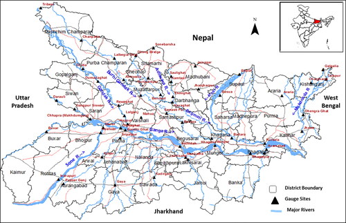
The study area is located between 24°20′10″ N to 27°31′15″ N and 83°19′50″ E to 88°17′40″ E (Figure 1). The region is bounded by the Himalayan foothills and Terai region of Nepal in the north and the Chota Nagpur plateau in the south. It forms part of the alluvial rich Indo-Gangetic plains, brought down by several rivers descending from northern side. The study area is divided into two halves by the River Ganges flowing from West to East. The major brunt of flood menace, is faced by North Bihar, because of higher population, exposure to floods, topography and higher rainfall in the upstream catchment areas (Jha and Gundimeda 2019; Matheswaran et al. 2019). About 76 per cent of North Bihar population is estimated to be living under the recurring flood threat (Flood Management Information System, n.d.). The south-west monsoon (June-September) contributes 80% to 90% of the total rainfall. The intense precipitation leads to higher runoff, causing most of the rivers to overflow and flood low lying areas adjoining to the flood plains. The recurrent flooding displaces millions of people, impacts their livelihoods, besides causing loss of lives, livestock and critical infrastructure (Bhatt et al. 2010; Singh et al. 2011; Manjusree et al. 2015; Mishra et al. 2019; Tripathi et al. 2019).

Figure 1. Location map of study area. Source: Author.

3. Data used and methodology

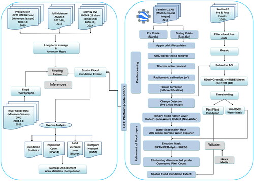
The flowchart of the entire process from GEE based SAR data processing (flood inundation extent), to assessment of flood proxy indicators (precipitation, soil moisture, vegetation indices and river gauge data), damage assessment (population impacted, agricultural land and transport network affected statistics) to inference making is presented in Figure 2.

Figure 2. Flowchart of methodology. Source: Author.

3.1. Primary and secondary data sources

Flood extent has been mapped using multi-temporal Sentinel-l SAR datasets acquired during flood season. The precipitation has been analyzed using data from Integrated Multi-satellite Retrievals (IMERG) of global precipitation mission (GPM), soil moisture from Advanced Microwave Scanning Radiometer-2 (AMSR-2), normalized difference vegetation index (NDVI) and enhanced vegetation index (EVI) from Moderate Resolution Imaging Spectroradiometer (MODIS). Further river gauge data obtained from the Central Water Commission (CWC) during the monsoon period was also used. The impact of flood event on population is assessed using gridded population data of the world (GPWv4), on agricultural land using land use/land cover data available from Bhuvan portal and on transport network using data from open street maps (OSM).

3.1.1. Sentinel-1 data for flood hazard mapping

For the present study the multi-temporal Sentinel-1 C (5.4 GHz) band Interferometric Wide (IW) swath mode Ground Range Detected (GRD) datasets from the Google Earth Engine (GEE) cloud computing platform (https://code.earthengine.google.com/) were processed for extraction of flood inundation footprints. Sentinel-1A & 1B Synthetic Aperture Radar (SAR) datasets from both ascending and descending passes and dual polarized (VV &VH) mode were processed. Level-1 GRD data consists of focused SAR data that are detected, multi-looked, and projected to the ground range using an Earth ellipsoid model. For 2019 about 35 scenes (13 in September and 22 in October months) were processed. In addition for comparative analysis of past inundation with 2019 event, data from 2017 about 31 scenes (15 in September and 16 in October) and 2018 about 29 scenes (15 in September and 14 in October) were also processed. Data from both the like-polarized (VV) and cross-polarized (VH) was used. Many studies in the past have suggested for utilization of both like and cross polarized data, because of co-polarized data’s sensitivity over the rough water surface and submerged agricultural fields (Henry et al. 2006; Manjusree et al. 2012; Clement et al. 2018; Ezzine et al. 2018). The datasets were accessed and processed using GEE based platform.

3.1.2. Integrated multi-satellite retrievals (IMERG) data for precipitation

For the assessment of precipitation, daily Final run data (3 months latency) with 0.1° × 0.1° spatial resolution retrieved by IMERG from global precipitation mission (GPM), was obtained from Goddard Earth Sciences Data and Information Services Center (GES DISC) website (https://disc.gsfc.nasa.gov). GPM-IMERG Final run data is considered to be the most accurate and reliable (Huffman et al. 2015a, b) as it also incorporates monthly rain-gauge analysis into account for its final estimation. The processed datasets were than stacked to generate long term (2000-18 & 2019) average weekly precipitation for the monsoon period (23^rd to 44^th week of the year) for further analysis.

3.1.3. Advanced microwave scanning radiometer 2 (AMSR-2) for soil moisture

Surface soil moisture data obtained by Advanced Microwave Scanning Radiometer 2 (AMSR-2) from both ascending and descending orbits, retrieved at 6.925 GHz channel by Land Parameter Retrieval Model (LPRM) was used. The dielectric property of the soil is strongly related to soil moisture and is expressed in percentage. The Level-3 gridded dataset for 2012-18 and 2019, with 10 km spatial resolution was downloaded from GES DISC website (https://disc.gsfc.nasa.gov) and further processed to generate long term average weekly precipitation for the monsoon period (23^rd to 44^th week of the year) for further analysis.

3.1.4. Moderate resolution imaging spectroradiometer (MODIS) data for NDVI and EVI

Normalized difference vegetation index (NDVI) and Enhanced vegetation index (EVI) was assessed using MODIS-AQUA observations. MYD13Q1 product was accessed from Land Processes Distributed Active Archive Center (LP DAAC) website (https://lpdaac.usgs.gov). Global MYD13Q1 data are provided every 16 days at 250-meter spatial resolution as a gridded level-3 product. NDVI is computed as the difference between near-infrared (NIR) and red (RED) reflectance divided by their sum (equation 1(1) $$\mathit{NDVI}=(\rho \mathit{NIR}-\rho R)/(\rho \mathit{NIR}+\rho R)$$(1) ), while the EVI is optimized to enhance the vegetation signal through a de-coupling of the canopy background signal (equation 2(2) $$\mathit{EVI}=G\left[\right(\rho \mathit{NIR}-\rho R)/\{\rho \mathit{NIR}+C_1(\rho R)-C_2\left(\rho B\right)+L\left\}\right]$$(2) ). (1) $$\mathit{NDVI}=(\rho \mathit{NIR}-\rho R)/(\rho \mathit{NIR}+\rho R)$$(1) (2) $$\mathit{EVI}=G\left[\right(\rho \mathit{NIR}-\rho R)/\{\rho \mathit{NIR}+C_1(\rho R)-C_2\left(\rho B\right)+L\left\}\right]$$(2) where,${\rho }_{\mathit{NIR}},$ ${\rho }_R$ and ${\rho }_B$ are the surface reflectance for the near-infrared, red and blue band respectively. $L$ is the canopy background adjustment ($L$ = 1), $C_1$ and $C_2$ are coefficients of the aerosol resistance term that uses blue band of MODIS to correct for aerosol influences in the red band ($C_1\mathrm{ }$= 6 and $C_2\mathrm{ }$= 7.5), and $G$ is a gain factor ($G$ = 2.5). The 16 days composite products for 2012-18 and 2019 for monsoon period were stacked to generate long term mean, extract vegetation indices and generate graphical plots for further analysis.

3.1.5. River gauge data for water level

Daily gauge-wise river water level data for monsoon period for last one decade span (2004-13) and for the flood event year, 2019 available from Central Water Commission (CWC) (http://cwc.gov.in/fmo/dfsra) was used in the analysis. River water level data for 27 gauge sites located along nine major river (Ganga, Kosi, Bagmati, Gandak, Ghaghara, Budhi Gandak, Kamala Balan, Adhwara and Mahananda) systems was used for generating flood hydrographs and understanding the seasonal onset and frequency of flooding. Based on the approach adopted by Dhar and Nandgiri (2000, 2002) river gauge data was also used for quantifying the flood and major flood incidences.

3.1.6. Other datasets for damage assessment

The gridded population count data (GPWv4) for 2020 at a resolution of 30 arc-seconds available from Socioeconomic Data and Applications Center (SEDAC) (https://sedac.ciesin.columbia.edu/) was integrated with the flooded layer to estimate the population impacted by the flooding using zonal statistics tool. The GPW datasets are extensively used for vulnerability and mapping of disaster impacts (Guha-Sapir et al. 2011). For assessing the transport network impacted, the open street maps (OSM) data (https://download.geofabrik.de/asia.html) was intersected with flood hazard layer. The agricultural damage was assessed using land use/land cover data available at Bhuvan portal (https://bhuvan-app1.nrsc.gov.in/state/BR).

3.2. Flood hazard mapping

3.2.1. Pre-processing

For flood hazard mapping pre-processing of Sentinel-1 SAR datasets, analysis and extraction of flood inundation layer, a customized script was run using Google Earth Engine (GEE) platform through GEE code editor (https://code.earthengine.google.com/). Radiometrically calibrated and terrain corrected Sentinel‐1 images are stored within GEE, which provides free cloud computing facilities for research . The datasets were accessed and pre-processed following the steps as demonstrated in Figure 2 to derive the terrain-corrected backscattering coefficient (σ°) images. Further, the images were filtered for the speckle noise that degrades the quality of the image using refined Lee speckle filter with a 3 × 3 window size. Finally, backscatter intensity was converted to backscatter coefficient (σ°) measured in decibels (dB as 10*log10σ°).

3.2.2. Backscattering analysis

In microwave domain water appears in dark tone as most of the radar energy goes away from the sensor due to specular reflection and therefore characterized by low radar backscatter response (Ulaby and Dobson 1989). The backscatter intensity values for pre-flood area varied between −14 and −19 dB for the VH polarization, and between −7 and −14 dB for the VV polarization. For the same areas during flood period backscatter intensity values varied between −26 and −33 dB approximately for VH polarization, and for VV between −17 and −26 dB. Due to flooding the backscatter intensity tends to decrease resulting in decrease towards even more negative values.

3.2.3. Flood inundation delineation

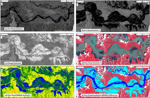
The flood inundated regions were delineated using the ratioing change detection method. For mapping and monitoring of the inundated regions using multi-temporal SAR images change detection techniques like the differencing and ratioing have been widely used (Martinez and Le Toan 2007; Herrera-Cruz et al. 2009; Schlaffer et al. 2015). Change detection methods have an advantage in eliminating out the permanent water bodies as compared to the methods which use single image (Twele et al. 2016). Using the ratioing approach (Singh 1989) the peak- flood mosaic images (Figure 3b) were divided by the pre-flood mosaic (Figure 3a) image intensity values (.divide operator) to deduce the changes per pixel (Figure 3c). The changes (flooded areas) are observed with brighter pixels, depending upon the degree of the changes between the two dates compared. The brighter pixels are than extracted using threshold operator (.gt(threshold) operator). Then through a trial and error approach optimal threshold (.gt(threshold) operator) is then adjusted depending in case of high rates of false positive or false negative values, by superimposing the classified binary raster layer generated, showing the flood extent over the crisis image. To check whether the change detection was performed accurately considering the threshold chosen, the usual practice has been in selecting arbitrary threshold values and testing them empirically (Nelson 1982). In the present study the threshold values varying between 1.15 and 1.30 were used. Pixels with values greater than the threshold were coded as 1 (flooded pixels) and other as 0 (non-flooded pixels).

Figure 3. GEE based (a) filtered mosaic of Sentinel-1 pre-flood, (b) during flood (flooded areas with darker tone), (c) ratio image (inundated areas with brighter tone) (d) cloud free during flood Sentinel-2 image, (e)classified flood water (dark blue) using NDWI and (f) validation with Sentinel derived approach (cyan colour). Source: Author.

3.2.4. Refining of flood inundation layer

The flooded layer was then further refined by removing the permanent water bodies. The Joint Research Centre (JRC) Global Surface Water Explorer “Seasonality” product (2018; 30 m resolution) accessed from https://global-surface-water.appspot.com/ was used to mask (.updatemask operator) the areas covered by water for > 10 months year⁻¹. For eliminating hill shadows Shuttle Radar Topography Mission (SRTM) digital elevation model (DEM) at 3 arc-seconds (ee.Algorithms.Terrain, operator) available from Hydro SHEDS (https://www.hydrosheds.org/) was used. Finally the isolated pixels were eliminated by finding the connectivity (.connectedPixelCount operator) of the flooded pixels. The final flood hazard layer was then further used for inundation statistics and damage assessment.

3.2.5. Validation of flood hazard layer

Sentinel-2B Level 1 C (spatial resolution 10 m) cloud free extent (over Ganga adjoining Munger, Begusarai and Bhagalpur districts) of optical data available (Figure 3d) was used for validation of Sentinel-1 derived flood spatial extent. The flood extent from Sentinel-2 (Figure 3e) derived using Normalized Difference Water Index (NDWI) approach (McFeeters 1996) was then superimposed over flood layer derived from Sentinel-1 data analysis (Figure 3f). In addition flood inundation was also cross checked based on the inundated areas reported from various sources available in open domain.

4. Results and discussions

4.1. Spatio-temporal pattern of precipitation

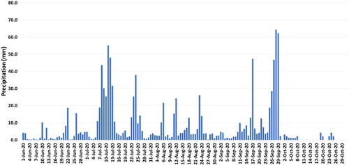
The spatio-temporal pattern of precipitation data analysis shows that during the 38^th and 39^th week of the year (second fortnight of September, 2019), Bihar witnessed 84 percent (254 mm) of the entire month’s precipitation (303 mm). A further closer look into the precipitation figures shows that about 64 percent (162 mm) of the total precipitation took place in the 39^th week itself against the long term average of about 59 mm (Figure 4). From the daily data analysis it was observed that during the 39^th week, the five days (25^th to 29^th September, 2019) of continuous heavy incessant precipitation, accounted for more than 50% of entire precipitation received during September (Figure 5). The spatial pattern of September rains during the second fortnight shows higher precipitation occurrence specifically over the central and the eastern regions of Bihar adjoining the Ganga River.

Figure 4. Graphical plot of temporal pattern of precipitation and soil moisture 22^nd to 44^th week for 2019 and long term average precipitation (2000-18) and soil moisture (2012-18) for the same period. Source: Author.

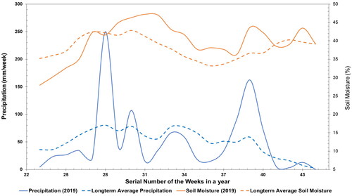
Figure 5. Graphical plot of GPM-IMERG (final run) based daily precipitation data during 2019. Source: Author.

4.2. Spatio-temporal changes in river gauge level

River gauge sites are very sensitive to precipitation variability, and therefore serves as an important proxy indicator of flooding. A river is said to be in flood situation when its water level crosses the danger level (DL) at that particular site. The river gauge data analysis shows attaining of peak water levels during late September to early October time frame by most of the river gauge sites located along the Ganga River (Table 1). Due to heavy precipitation during the 39^th week of the year (late September, 2019) specifically over central parts of Bihar, most of the rivers gauge sites (Dighaghat, Gandhighat and Hatidah in Patna district, Munger site in Munger district, Bhagalpur and Kahalgaon sites in Bhagalpur district) located along Ganga River started overflowing and remained to be in spate for almost two weeks (early October; 40^th week of the year) recording higher water levels. Gauge sites located at Bhagalpur, Hathidah and Kahalgaon were observed to have attained water levels only 0.5 m below the previous ever recorded highest flood levels (HFL). In addition few other gauge sites located along the confluence of Ganga River like Kursela (Kosi River) and Khagaria (Burhi Gandak) were also observed to be in spate.

Table 1. Gauge sites with their danger level, high flood level and maximum water level attained during 2019 flood season.

S.No	River	Gauge Site	Danger Level (DL) (m)	High Flood Level (HFL) (m)	Date of HFL Occurrence	Maximum Water Level (MWL) 2019 Sept-Oct	Date of MWL Occurrence	Deviation From DL(m)	Deviation From HFL(m)
1	Ganga	Dighaghat	50.45	52.52	23-Aug-75	50.94	23-Sep-19	0.49	−1.58
		Gandhighat	48.6	50.52	21-Aug-16	49.79	24-Sep-19	1.19	−0.73
		Hathidah	41.76	43.17	21-Aug-16	42.75	25-Sep-19	0.99	−0.42
		Munger	39.33	40.99	19-Sep-76	39.59	2-Oct-19	0.26	−1.4
		Bhagalpur	33.68	34.72	26-Aug-16	34.43	2-Oct-19	0.75	−0.29
		Kahalgaon	31.09	32.87	17-Sep-03	32.36	3-Oct-19	1.27	−0.51
2	Kosi	Kursela	30	32.04	6-Sep-98	31.6	1-Oct-19	1.6	−0.44
		Baltara	33.85	36.4	15-Aug-87	35.59	17-Jul-19	1.74	−0.81
		Basua	47.75	49.24	13-Aug-17	48.08	19-Sep-19	0.33	−1.16
3	Bagmathi	Hayaghat	45.72	48.96	14-Aug-87	46.71	28-Jul-19	0.99	−2.25
		Benibad	48.68	50.01	12-Jul-04	49.1	18-Jul-19	0.42	−0.91
		Hajipur	50.32	50.93	18-Aug-48	49.78	21-Sep-19	−0.54	−1.15
4	Gandak	Rewaghat	54.51	55.41	17-Sep-86	53.75	20-Sep-19	−0.76	−1.66
		Chatia	69.15	70.04	26-Jul-02	–	–	–	–
		Chappra	53.68	54.59	3-Sep-02	53.25	24-Sep-19	−0.43	−1.34
5	Ghaghara	Gangpur Siswan	57.04	58.01	18-Sep-83	57.36	23-Sep-19	0.32	−0.65
		Darauli	60.82	61.74	29-Aug-98	60.86	22-Sep-19	0.04	−0.88
		Khagaria	36.58	39.22	16-Aug-76	38.28	2-Oct-19	1.7	−0.94
		Rusera	42.63	46.35	16-Aug-87	44.12	23-Jul-19	1.49	−2.23
6	Budhi Gandak	Samastipur	46.02	49.38	15-Aug-87	47.26	30-Jul-19	1.24	−2.12
		Sikandarpur	52.53	54.29	15-Aug-87	52.69	21-Jul-19	0.16	−1.6
		Lalbegia Ghat	63.2	67.09	30-Jul-75	63.6	19-Jul-19	0.4	−3.49
7	Kamala Balan	Jhanjharpur	50	52.67	12-Aug-87	51.24	17-Jul-19	1.24	−1.43
		Ekmighat	46.94	49.27	14-Aug-87	47.91	29-Jul-19	0.97	−1.36
8	Adhawara	Kamtaul	50	52.99	14-Aug-87	51.27	17-Jul-19	1.27	−1.72
		Dhengraghat	35.65	38.2	14-Aug-17	36.9	17-Jul-19	1.25	−1.3
9	Mahananda	Jhawa	31.4	34.07	14-Aug-17	33.89	17-Jul-19	2.49	−0.18

4.3. Spatio-temporal pattern of soil moisture

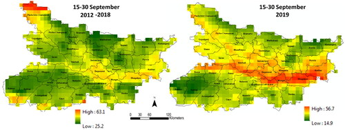
The higher precipitation activity observed in late September, 2019 especially around 39^th week is reflected in the form of an increased soil moisture build up. The increase is observed particularly during the 39^th and the 40^th week of about 19 and 15 percent higher than the long term soil moisture (Figure 4). The soil moisture build up is well captured spatially also and clearly appears to be higher particularly in the central and eastern districts (Bhojpur, Patna, Vaishali, Lakhisarai, Munger, Khagaria, Bhagalpur, Katihar, Purnia, Darbhanga, Muzaffarpur, Siwan and Saran) as compared to the long term soil moisture for the same period (Figure 6).

Figure 6. Spatial representation of soil moisture from AMSR-2 data for late September, 2019 floods compared with long term average (2012-18) for same time frame. Source: Author.

4.4. Spatio-temporal changes in NDVI and EVI

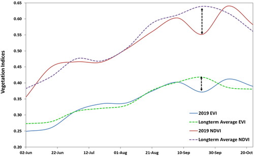
The assessment of multi-temporal spectral response using vegetation indices such as the normalized difference vegetation index (NDVI) and enhanced vegetation index (EVI) helps to detect the changes in vegetation induced due to flooding hazard (Džubáková et al. 2015; Kwak et al. 2015). The vegetation indices values ranges from − 1.0 to +1.0, negative values indicate the presence of water, and the positive values are correlated with green vegetation. From the analysis of 16 days composite MODIS product a sharp dip in NDVI and EVI values is observed during September 2019 (39^th week) as compared to the long term average. The decrease in MODIS-NDVI and EVI response detected in around 39^th week is associated with the accumulation of floodwaters. Shrestha et al. (2013) and Kwak et al. (2015) have also observed drop in NDVI and EVI response of the vegetation during the flood event as compared to the non-flooding conditions. In the present analysis the NDVI and EVI values have dropped by 13.7 percent and 11.1 percent respectively around September 22, 2019 from the long term average values (Figure 7).

Figure 7. Graphical plot of NDVI and EVI vegetation indices values for 2019 during flood season compared with the long run (2000-18) average for same time frame. Source: Author.

4.5. Spatio-temporal analysis of flood event

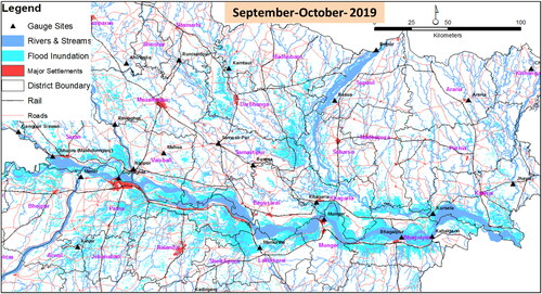
The spatio-temporal analysis of flood inundation extent was analyzed from the multi-temporal C-band Sentinel-1 datasets. The analysis showed that during the first half (36^th & 37^th week) of September, 2019 about 1.13 lakh ha of area was under submergence. However, during the second fortnight (38^th & 39^th week) of September, 2019 the flooded area increased by ∼82 percent (6.17 lakh ha). The flooded area further increased to 8.05 lakh ha during the first fortnight of October, 2019 (40^th-41^st week). Thereafter, a significant recession in flooding was observed. The cumulative spatial extent of flooding (Figure 8) during the peak flooding period between second fortnight of September and first fortnight (38^th to 41^st week) of October, 2019 was observed to be about 9.23 lakh ha (9.7 percent of states total geographical area), whereas about 4.99 lakh ha of area remained impacted in both time frames. The peak flooding impacted about 4.5 percent of states cropped area, about 1395 km of road network and 115 km of rail network during this period. Out of the total 38 districts in Bihar state, 18 districts especially in the central and eastern parts, adjoining the flood plains of the Ganga River on the north and south banks had more than 10 percent of their districts geographical area (DGA) inundated. Bhagalpur (35.8% of DGA), Patna (30.2% of DGA) followed by Khagaria (26.9% of DGA), Lakhisarai (26.4% of DGA) and Munger (21.7% of DGA) were the worst affected districts. About 9.26 million population was assessed to be affected, with Patna (1.45 million people) followed by Bhagalpur district (0.69 million people) contributing to the highest population affected by the late September flood wave. The 2019 late September flooding event also provided a conducive environment to the spread of water borne diseases especially in Patna which witnessed a high rise in dengue fever cases.

Figure 8. Cumulative spatial extent of flood inundation during September-October, 2019. Source: Author.

4. Discussion

The precipitation data processed for last 19 years (2000–2018) from GPM-IMERG for the monsoon months (23^rd-44^th week of the year) shows that monsoon rain starts in Bihar from June onwards (∼23^rd -26^th weeks), with July (∼27^th -30^th weeks) and August (∼31^st -35^th weeks) being the months of maximum precipitation activity, followed by September (∼36^th -39^th weeks). A further closer look into the precipitation shows that major precipitation spell windows during monsoons are during July from second to last week (29^th-31^st week of the year), whereas in August it is from mid to last week (34^th-35^th week of the year) and in September it is confined to the first half (36^th-37^th week of the year) and thereafter there is continuous recession in precipitation activity (Figure 4). However, during 2019 precipitation pattern has shown a substantial deviation both in amount of precipitation received as compared to the long term average and also in temporal pattern of occurrence. Here it is also interesting to observe that between 31^st and 36^th weeks (August month) the precipitation was below normal, which is in general the peak monsoon precipitation and flooding period. From the IMERG data analyzed for 2019 it is clearly observed that during the 2019 monsoon season between 23^rd (early-June) and 37^th week (mid-September), Bihar had received 748 mm rainfall against the corresponding 919 mm (long term average) amounting to almost 18 percent rain deficit. However, consecutive heavy spells of precipitation towards the end of September (38^th and 39^th weeks) changed the situation from deficit to surplus. The excessive heavy spell in particular during the 39^th week concentrated between 25^th and 29^th September, contributing to almost 50 percent of entire September month’s precipitation, changed the situation from deficit to a surplus of almost 2.5 percent, causing widespread flooding. Sunitha Devi et al. (2019) have explained the delayed retreat of south-west monsoon up to 1^st week of October in 2019, due to the prevalence of an active Inter Tropical Convergence Zone, across central India, North Indian Ocean, extending up to western North Pacific Ocean.

From the long term soil moisture data it can be observed that after initial monsoon peak rainfall around 28^th week (mid-July) the soil moisture build up started peaking up till 32^nd week (mid-August) and thereafter a continuous decline is registered until another peak rainfall peak around 39^th week (Figure 4). Though the precipitation after July has been below normal but due to the initial heavy precipitation activity the moisture has been able to maintain above normal though on a declining trend. However, the higher soil moisture conditions during the 39^th and 40^th weeks preceded by a heavy precipitation (38^th and 39^th weeks) event lead to higher surface runoff and, consequently aggravating the severity of flooding associated with the rainfall event. The soil moisture map derived from the last 19 years data clearly shows relatively lower soil moisture in the central and eastern districts of Bihar during the latter half of September, as compared to that observed in 2019 which displayed a substantially higher moisture content (Figure 6). The 2019 late September floods disaster footprints spatial extent is assessed to be far higher in comparison to the previous 2017 and 2018 for the same period. The area under submergence shows almost 7-8 times increase in latter half of September and 12-15 times in first half of October during 2019 as compared to 2017 and 2018. The multi-temporal EVI and NDVI profiles highly correlated with the changes in the soil moisture and river water levels. The intense precipitation activity leading to increase in moisture buildup and consequent accumulation of flood has equally been represented through a significant dip in the value of vegetation indices like NDVI and EVI. Due to poor soil aeration conditions of flooded soils adversely affects the plant growth.

The month-wise break up of last one decade gauge data shows that 22% of the flood incidences occur in July, about 46% occur in August month, 27% in September and 5% in October. The month-wise gauge data analysis clearly highlights the fact that though precipitation is active in July, but it is mainly utilized in fulfilling the initial soil moisture deficit and as the monsoon intensifies and the soils get fully saturated to their full capacity, the excess rain water appears as surface runoff and resulting in severe flooding especially in August month. A perusal of Table 1 clearly shows that out of the 27 gauge sites long term gauge data analyzed, the highest ever recorded water level for 18 sites is attained during the month of August, 6 sites in September and 3 in July month. It is also to be observed that the HFL attained during September month are confined to the first fortnight, thereby clearly indicating recession in the flooding intensity in the latter half of September. However, from the 2019 flood season gauge data analysis it is observed that July had 33%, September 36%, October 21% whereas August only contributing to 10% of the total flood incidences in 2019. The preceding gauge data analysis not only confirms to the heavy precipitation and flooding incidences observed in September and October 2019, but also highlights the recession in peak flooding activity in August with an increase in July month unlike observed from long range data observations.

5. Conclusions

The present study based on the integrated space and ground based observations has very aptly been able to capture the late September 2019 triggered flood disaster footprints and comprehend the changes of flooding through various space and ground flood proxy indicators. The long term data analysis of precipitation, soil moisture, vegetation and river gauge data is clearly able to highlight the flood anomaly, triggered due to the prolonging of monsoon season in 2019. The 2019 delayed monsoon withdrawal and excessive late September rains causing floods in most of North India, has led to the computation of new withdrawal dates for monsoons operational services considering climatological data from 1961 to 2019 against the old data earlier used 1901–1940 (Pai et al. 2020). The onset of monsoons is now one week before the existing normal but the monsoon withdrawal from northwest India is delayed by more than two weeks compared to the existing normal date (i.e., 1^st September). The precipitation and river gauge data long term analysis also bring out an interesting observation wherein a gradual decline in the flooding events is observed in the month of August as compared to the past. Therefore the present analysis can be important input for policy makers for adapting to the changing flood pattern and better preparedness to deal with disaster response and flood mitigation activities in future. The above observations also necessitate specifically for adopting to strategies to newer cropping patterns and controlling spread of water borne diseases which get impacted due to accumulation of flood waters. This study also highlights that precipitation, soil moisture, vegetation indices are very good and sensitive proxy indicators of flooding and therefore can very well complement the direct satellite based captured flood disaster footprints. The potential of openly available earth observation data combined with cloud computing platforms today can be an important tool for rapid assessment of the situation and informed decision making.

Acknowledgements

The authors would like to thank the anonymous reviewers for their helpful comments and constructive suggestions. Authors would also like to thankfully acknowledge all the portals (LP DAAC, GES DISC, CWC, OSM and CIESIN) and platforms (GEE) through which the data/products have been accessed and analyzed for the present study.

Disclosure statement

No potential conflict of interest was reported by the authors.

Correction Statement

This article has been republished with minor changes. These changes do not impact the academic content of the article.

References

- Ahlmer AK, Cavalli M, Hansson K, Koutsouris AJ, Crema S, Kalantari Z. 2018. Soil moisture remote-sensing applications for identification of flood-prone areas along transport infrastructure. Environ Earth Sci. 77(14):533.
- Amarnath G, Matheswaran K, Pandey P, Alahacoon N, Yoshimoto S. 2017. Flood mapping tools for disaster preparedness and emergency response using satellite data and hydrodynamic models: a case study of Bagmathi Basin, India. Proc Natl Acad Sci India, Sect A Phys Sci. 87(4):941–950.
- Berezowski T, Bielinski T, Osowicki J. 2020. Flooding extent mapping for synthetic aperture radar time series using river gauge observations. IEEE J Sel Top Appl Earth Obs Remote Sens. 13:2626–2638.
- Bhatt CM, Rao GS. 2016. Ganga floods of 2010 in Uttar Pradesh, north India: a perspective analysis using satellite remote sensing data. Geomatics Nat Hazards Risk. 7(2):747–763.
- Bhatt CM, Rao GS, Farooq M, Manjusree P, Shukla A, Sharma SVSP, Kulkarni SS, Begum A, Bhanumurthy V, Diwakar PG, et al. 2017. Satellite-based assessment of the catastrophic Jhelum floods of September 2014, Jammu & Kashmir, India. Geomatics Nat Hazards Risk. 8 (2):309–327..
- Bhatt CM, Rao GS, Manjushree P, Bhanumurthy V. 2010. Space based disaster management of 2008 Kosi floods, North Bihar, India. J Indian Soc Remote Sens. 38(1):99–108.
- Borah SB, Sivasankar T, Ramya MNS, Raju PLN. 2018. Flood inundation mapping and monitoring in Kaziranga National Park, Assam using Sentinel-1 SAR data. Environ Monit Assess. 190(9):520.
- Canty MJ, Nielsen AA, Conradsen K, Skriver H. 2020. Statistical analysis of changes in Sentinel-1 time series on the google earth engine. Remote Sens. 12(1):46.
- Clement MA, Kilsby CG, Moore P. 2018. Multi‐temporal synthetic aperture radar flood mapping using change detection. J Flood Risk Manage. 11(2):152–168.
- Dhar ON, Nandargi S. 2000. A study of floods in the Brahmaputra Basin in India. Int J Climatol. 20(7):771–781. AID-JOC518 > 3.0.CO;2-Z
- Dhar ON, Nandargi S. 2002. Flood study of the Himalayan tributaries of the Ganga River. Meteorol Appl. 9(1):63–68. https://doi.org/doi/pdf/10.1017/S135048270200107X
- Džubáková K, Molnar P, Schindler K, Trizna M. 2015. Monitoring of riparian vegetation response to flood disturbances using terrestrial photography. Hydrol Earth Syst Sci. 19(1):195–208.
- ESA Sentinel Online. User guides and technical guides of Sentinel-1 SAR. [accessed 2020 Jun 8]. Available from: https://sentinel.esa.int/web/sentinel/user-guides/sentinel-1-sar
- Ezzine A, Darragi F, Rajhi H, Ghatassi A. 2018. Evaluation of Sentinel-1 data for flood mapping in the upstream of Sidi Salem dam (Northern Tunisia). Arab J Geosci. 11(8):170.
- Flood Management Information System. (n.d.). History of flood. [accessed 26 June 2019]. Available from: http://fmis.bih.nic.in/history.html.
- Gorelick N, Hancher M, Dixon M, Ilyushchenko S, Thau D, Moore R. 2017. Google Earth Engine: Planetary-scale geospatial analysis for everyone. Remote Sens Environ. 202:18–27..
- Guha-Sapir D, Rodriguez-Llanes JM, Jakubicka T. 2011. Using disaster footprints, population databases and GIS to overcome persistent problems for human impact assessment in flood events. Nat Hazards. 58(3):845–852.
- Guhathakurta P, Sreejith OP, Menon PA. 2011. Impact of climate change on extreme rainfall events and flood risk in India. J Earth Syst Sci. 120(3):359–373.
- Henry JB, Chastanet P, Fellah K, Desnos YL. 2006. Envisat multi‐polarized ASAR data for flood mapping. Int J Remote Sens. 27(10):1921–1929.
- Herrera-Cruz V, Koudogbo F, Herrera V. 2009. TerraSAR-X rapid mapping for flood events. Proceedings of the International Society for Photogrammetry and Remote Sensing (Earth Imaging for Geospatial Information), Hannover, Germany, p. 170–175.
- Ho-Hagemann HTM, Hagemann S, Rockel B. 2015. On the role of soil moisture in the generation of heavy rainfall during the Oder flood event in July 1997. Tellus A: Dyn Meteorol Oceanogr. 67(1):28661.
- Huffman GJ, Bolvin DT, Braithwaite D, Hsu K, Joyce R, Xie P, Yoo SH. 2015. NASA global precipitation measurement (GPM) integrated multi-satellite retrievals for GPM (IMERG). Algorithm Theor Basis Doc (ATBD) Version. 4:26.
- Huffman GJ, Bolvin DT, Nelkin EJ. 2015. Integrated multi-satellite retrievals for GPM (IMERG) technical documentation. NASA/GSFC Code. 612(2015):47.
- Jena PP, Chatterjee C, Pradhan G, Mishra A. 2014. Are recent frequent high floods in Mahanadi basin in eastern India due to increase in extreme rainfalls? J Hydrol. 517:847–862..
- Jha RK, Gundimeda H. 2019. An integrated assessment of vulnerability to floods using composite index–A district level analysis for Bihar, India. Int J Disaster Risk Reduct. 35:101074..
- Kwak Y, Arifuzzanman B, Iwami Y. 2015. Prompt proxy mapping of flood damaged rice fields using MODIS-derived indices. Remote Sens. 7(12):15969–15988..
- Lal P, Prakash A, Kumar A. 2020. Google Earth Engine for concurrent flood monitoring in the lower basin of Indo-Gangetic-Brahmaputra plains. Nat Hazards. :. 104(2): 1947–1952.
- Manjusree P, Bhatt CM, Begum A, Rao GS, Bhanumurthy V. 2015. A decadal historical satellite data analysis for flood hazard evaluation: a case study of Bihar (North India). Singap J Trop Geogr. 36(3):308–323.
- Manjusree P, Kumar LP, Bhatt CM, Rao GS, Bhanumurthy V. 2012. Optimization of threshold ranges for rapid flood inundation mapping by evaluating backscatter profiles of high incidence angle SAR images. Int J Disaster Risk Sci. 3(2):113–122.
- Martinez JM, Le Toan T. 2007. Mapping of flood dynamics and spatial distribution of vegetation in the Amazon floodplain using multitemporal SAR data. Remote Sens Environ. 108(3):209–223.
- Matheswaran K, Alahacoon N, Pandey R, Amarnath G. 2019. Flood risk assessment in South Asia to prioritize flood index insurance applications in Bihar, India. Geomatics Nat Hazards Risk. 10(1):26–48.
- McFeeters SK. 1996. The use of the Normalized Difference Water Index (NDWI) in the delineation of open water features. Int J Remote Sens. 17(7):1425–1432.
- Mishra V, Aaadhar S, Shah H, Kumar R, Pattanaik DR, Tiwari AD. 2018. The Kerala flood of 2018: combined impact of extreme rainfall and reservoir storage. Hydrol Earth Syst Sci Discuss. 1–13. doi: https://doi.org/10.5194/hess-2018-480
- Mishra AK, Meer MS, Nagaraju V. 2019. Satellite-based monitoring of recent heavy flooding over north-eastern states of India in July 2019. Nat Hazards. 97(3):1407–1412..
- Mishra K, Sinha R. 2020. Flood risk assessment in the Kosi megafan using multi-criteria decision analysis: A hydro-geomorphic approach. Geomorphology. 350:106861.
- Nelson RF. 1982. Detecting forest canopy change using Landsat. NASA technical memorandum 83918. Greenbelt, MD: Goddard Space Flight Centre.
- Pai DS, Bandgar A, Devi S, Musale M, Badwaik MR, Kundale AP, Gadgil S, Mohapatra M, Rajeevan M. 2020. New normal dates of onset/progress and withdrawal of southwest monsoon over India. [accessed 2020 Jun 15]. https://internal.imd.gov.in/press_release/20200515_pr_804.pdf.
- Pandey RK, Crétaux JF, Bergé-Nguyen M, Tiwari VM, Drolon V, Papa F, Calmant S. 2014. Water level estimation by remote sensing for the 2008 flooding of the Kosi River. Int J Remote Sens. 35(2):424–440.
- Prasad AK, Kumar VK, Singh S, Singh RP. 2006. Potentiality of multi-sensor satellite data in mapping flood hazard. J Indian Soc Remote Sens. 34(3):219–231..
- Prasad AK, Singh S, Singh RP. 2005. Extreme rainfall event of July 25–27, 2005 over Mumbai, West Coast, India. J Indian Soc Remote Sens. 33(3):365–370..
- Ray K, Pandey P, Pandey C, Dimri AP, Kishore K. 2019. On the recent floods in India. Current Science. 117(2):204.
- Schlaffer S, Matgen P, Hollaus M, Wagner W. 2015. Flood detection from multi-temporal SAR data using harmonic analysis and change detection. Int J Appl Earth Obs Geoinf. 38:15–24.
- Shrestha R, Di L, Yu G, Shao Y, Kang L, Zhang B. 2013 Aug. Detection of flood and its impact on crops using NDVI-Corn case. In 2013 Second International Conference on Agro-Geoinformatics (Agro-Geoinformatics). IEEE; p. 200–204.
- Singh RP, Kumar R, Tare V. 2009. Variability of soil wetness and its relation with floods over the Indian subcontinent. Can J Remote Sens. 35(1):85–97.
- Singh A. 1989. Review article digital change detection techniques using remotely-sensed data. Int J Remote Sens. 10(6):989–1003..
- Singha M, Dong J, Sarmah S, You N, Zhou Y, Zhang G, Doughty R, Xiao X. 2020. Identifying floods and flood-affected paddy rice fields in Bangladesh based on Sentinel-1 imagery and Google Earth Engine. ISPRS J Photogramm Remote Sens. 166:278–293.
- Singh SK, Pandey AC, Nathawat MS. 2011. Rainfall variability and spatio temporal dynamics of flood inundation during the 2008 Kosi flood in Bihar State. Asian J Earth Sci. 4(1):9–19.
- Sinha R, Bapalu GV, Singh LK, Rath B. 2008. Flood risk analysis in the Kosi river basin, north Bihar using multi-parametric approach of analytical hierarchy process (AHP). J Indian Soc Remote Sens. 36(4):335–349.
- Sunitha Devi S, Krishna Mishra SP, Singh NK, Kashyapi A, Sathi Devi K. 2019. Regional characteristics of the south-west monsoon. [accessed 2020 Sep 20]. http://www.imdpune.gov.in/Clim_Pred_LRF_New/Reports/Monsoon_Report_2019/Chapter_1.pdf.
- Tiwari V, Kumar V, Matin MA, Thapa A, Ellenburg WL, Gupta N, Thapa S. 2020. Flood inundation mapping- Kerala 2018; harnessing the power of SAR, automatic threshold detection method and Google Earth Engine. Plos One. 15(8):e0237324.
- Tripathi G, Pandey AC, Parida BR, Shakya A. 2020. Comparative flood inundation mapping utilizing multi-temporal optical and SAR satellite data over North Bihar region: a case study of 2019 flooding event over North Bihar. In: Spatial information science for natural resource management. IGI Global Publisher of Timely Knowledge; p. 149–168. doi: https://doi.org/10.4018/978-1-7998-5027-4.ch008. https://www.igi-global.com/chapter/comparative-flood-inundation-mapping-utilizing-multi-temporal-optical-and-sar-satellite-data-over-north-bihar-region/257701
- Tripathi G, Parida BR, Pandey AC. 2019. Spatio-temporal rainfall variability and flood prognosis analysis using satellite data over North Bihar during the August 2017 flood event. Hydrology. 6(2):38..
- Twele A, Cao W, Plank S, Martinis S. 2016. Sentinel-1-based flood mapping: a fully automated processing chain. Int J Remote Sens. 37(13):2990–3004.
- Uddin K, Matin MA, Meyer FJ. 2019. Operational flood mapping using multi-temporal sentinel-1 SAR images: a case study from Bangladesh. Remote Sens. 11(13):1581.
- Ulaby FT, MC. Dobson. 1989. Handbook of radar scattering statistics for terrain. Norwood, MA: Artech House.
- Vanama VSK, Mandal D, Rao YS. 2020. GEE4FLOOD: rapid mapping of flood areas using temporal Sentinel-1 SAR images with Google Earth Engine cloud platform. J Appl Rem Sens. 14(03):1.
- Vishnu CL, Sajinkumar KS, Oommen T, Coffman RA, Thrivikramji KP, Rani VR, Keerthy S. 2019. Satellite-based assessment of the August 2018 flood in parts of Kerala, India. Geomatics Nat Hazards Risk. 10(1):758–767..
- Wang L, Diao C, Xian G, Yin D, Lu Y, Zou S, Erickson TA. 2020. A summary of the special issue on remote sensing of land change science with Google earth engine. Remote Sens Environ. 248:112002..
- Yuan F, Zhang L, Soe KMW, Ren L, Zhao C, Zhu Y, Jiang S, Liu Y. 2019. Applications of TRMM-and GPM-Era multiple-satellite precipitation products for flood simulations at sub-daily scales in a sparsely gauged watershed in Myanmar. Remote Sens. 11(2):140.