Multi-hazard risk mapping for coupling of natural and technological hazards

Abstract

Technological hazards induced by natural hazards have a significant impact on human life and economy. Their power exceeds the impact of the natural hazards that caused them. However, most of the multi-hazard risk maps failed to incorporate technological hazards when mapping multi hazard risk. To address this problem, we established a hybrid multi-hazard risk assessment methodology that calculates the risk caused by natural and technological hazards in a three-step process. First, the possible natural and technological hazards in a given region are identified by hazard-forming environment analysis and hazard source investigation respectively. A scenario simulation is adopted to analyze the intensity and impact scope of these hazards. Second, the triggered relationships among natural and technological hazards are analyzed by a hazard matrix. Then, the radar graph is adopted to calculate the multi-hazard intensity under the coupling effect of all possible hazards in this region. Third, the multi-hazard risk is calculated by aggregating land use data and multi-hazard intensity together. This methodology was applied in Huairou Science City (HSC), Beijing. The result shows that the joint action of earthquake and liquid ammonia leakage is the main reason for the high risk in the central area of HSC. The methodology developed in this study can clearly show the different impacts of each hazard on a given region under the action of hazard coupling, and the calculated results can better reflect the actual disaster situation.

Keywords:

• Multi-hazard risk
• hazard interaction
• natural hazard
• technological hazard
• radar graph

1. Introduction

Multi-hazard risk refers to the risk arising from multiple hazards (Kappes et al. 2012; Aksha et al. 2020; Gautam et al. 2021). In principle, it accounts for the characteristics of each hazardous event (e.g. probability, frequency, magnitude), and their mutual interactions and interrelations (e.g. one hazard may occur repeatedly in time; different hazards may independently occur at the same place; different hazards may occur dependently at the same place) (Kappes et al. 2012; Marzocchi et al. 2012; Gallina et al. 2016). A multi-hazard risk map is an operational risk management tool that utilizes graphic technology to represent the identified multi-hazard risk information and visualize the development trend of risks (Kappes et al. 2012; Komendantova et al. 2014; Bathrellos et al. 2017). Since it can support the decision-making process of risk managers, it is widely applied in risk management area (Buck and Summers 2020; Pourghasemi et al. 2020).

Despite the huge amount of studies in multi-hazard risk mapping (Gallina et al. 2016; Liu et al. 2016a; Zscheischler et al. 2018), most of them merely focused on the risk induced by natural hazards, and ignored technological hazards (Barrantes 2018; Dabbeek and Silva 2020; Sutanto et al. 2020). In fact, many natural hazards have the potential to trigger technological hazards, e.g. fires, explosions and leakage of toxic or radioactive materials (Girgin et al. 2019; He and Weng 2020). These technological hazards can severely affect human life and economy, and in some cases, their impact can exceed the impact of the natural hazards that caused them (Schmidt-Thomé 2006; Chen et al. 2019; Girgin et al. 2019). For example, the occurrence of 2011 Tohoku earthquake and tsunami has triggered the meltdown of three reactors in the Fukushima Daiichi Nuclear Power Plant complex. The influence scope and duration of the nuclear leakage have exceeded those of the earthquake and tsunami (Norio et al. 2011). Therefore, in order to reduce risk, it is important to incorporate technological hazards into multi-hazard risk mapping.

Hazard interactions and interrelations analysis is the key for multi-hazard risk mapping (Tilloy et al. 2019). Previous investigations on coupling effect of natural and technological hazards mainly concentrated on the domino effect, and mostly performed event tree analysis (Marzocchi et al. 2012; Gill and Malamud 2014; Eshrati et al. 2015). Such an approach generally analyses hazard interaction that begins with given information about one primary hazard, which triggers or increases the probability of others hazards (Liu et al. 2016b). However, the interaction between different hazards is complex and dynamic, thus it is difficult to cover all situations using the linear relationship of domino effect (Liu et al. 2017; Tilloy et al. 2019). For example, natural and technological hazards may occur independently without evident common cause, but in close proximity, spatially, temporally, or both. Hence, it is difficult to map multi-hazard risk and reflect the actual disaster situation by fully relying on the domino effect analysis. Therefore, this paper aims to develop a hybrid multi-hazard risk assessment methodology to map the risk caused by natural and technological hazards, with an explicit consideration of coupling effect between all possible natural and technological hazards.

2. Methodology

2.1. Framework

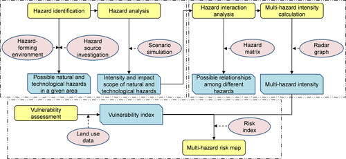
The main aim of this paper is to develop a methodology for mapping multi-hazard risk of coupling of natural and technological hazards. The basic structure of this methodology is shown in Figure 1. The first step is to identify the possible natural and technological hazards in a given area, and analyze the intensity and impact scope of these hazards using scenario simulation method. In the second step, the overlapping areas of different hazards are identified using ArcGIS. By analyzing the possible relationships among these hazards using hazard matrix, radar graph is adopted to calculate and display the multi-hazard intensity. In the third step, land use data is selected to characterize vulnerability. A Multi-hazard risk map is drawn by combining land use data and multi-hazard intensity together.

Figure 1. Framework for mapping multi-hazard risk of coupling of natural and technological hazards.

2.2. Hazard identification and analysis

In this step, natural hazards are first identified based on the hazard-forming environment. Environmental factors in the specific geophysical environment determine the preconditions for the occurrence of a specific natural hazard (Liu et al. 2016b). According to the characteristics of these environmental factors, the spatial distribution of natural hazards in a region can be deduced. Then the historical data is adopted to simulate the possible impact scope and the corresponding intensity of these hazards, e.g. Grünthal et al. (2006) simulated the inundation area and flood depth in Cologne by historic flood events. Technological hazards are identified by investigating the source of hazards, e.g. inventories of flammable and explosive materials. Then, the related models are adopted to calculate the impact scope and the corresponding intensity of technological hazards based on the hazardous material reserves, e.g. TNT equivalent method for calculating the impact scope and intensity of explosion (He and Weng 2020). Finally, the intensity of every single hazard is divided into six different intensity levels from 0 to 5. The higher the number, the greater the hazard intensity. Number 0 means that the hazard has no impact on this area.

2.3. Hazard interaction analysis

The triggered relationships among different hazards are summarized by a hazard matrix as shown in Figure 2 (Gill and Malamud 2014; Liu et al. 2016b), where hazards are categorized into natural (green) and technological (red). The vertical axis of the matrix shows the primary hazards, i.e. the initial hazards that trigger other hazards. The horizontal axis shows the potential secondary hazards, i.e. the hazards induced by initial hazards. Dark blue in the cell indicates that the primary hazard has a high probability to induce the secondary hazard. Light blue indicates that the primary hazard has a low probability of inducing secondary hazard. White indicates no obvious trigger relationship between the two hazards.

Figure 2. Hazard matrix for triggered relationships among different hazards.

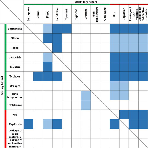
Figure 2 illustrates that most of the natural hazards have a certain probability of inducing technological hazards. 1) When an earthquake is a primary hazard, it could induce floods, tsunamis, landslides, fires, explosions, leakage of toxic materials and leakage of radioactive materials. There is a certain probability that earthquakes would result in the destruction of dams, which would cause the overflow of river and flooding (Dai et al. 2005). When an earthquake occurs on the seafloor, the abrupt rise and fall of the seabed topography would bring strong disturbance to the ocean, and there is a certain probability that it would trigger a tsunami (Norio et al. 2011). Earthquakes can easily change the stability of the slope, and it is more likely to induce landslides in a hilly area (Xie et al. 2018). There is a high probability that earthquakes would damage buildings, and cause the leakage of flammable and explosive materials, toxic materials and radioactive materials (Girgin et al. 2019). Among them, flammable and explosive materials are prone to fire or even explosion when encountering open flames (He and Weng 2020). 2) When a storm or typhoon is the primary hazard, heavy rainfall could lead to severe floods and landslides. Floods, landslides, strong winds and heavy rainfall could damage buildings, which could lead to fires, explosions and leakage of toxic or radioactive materials (Zeng et al. 2021). 3) When high temperature or drought is the primary hazard, continuous high temperature and dry climate would increase the possibility of fire and explosion (Satir et al. 2016). 4) When fire or explosion is the primary hazard, there is a certain probability that the explosion would damage the building and cause the leakage of toxic or radioactive materials (He and Weng 2020). In addition, the explosion could damage the dam and result in flooding, as well as change the stability of the slope to induce landslides.

The possible impact scope for every single hazard is identified in the hazard identification and analysis section. In this step, the overlapping area of different hazards is identified by synthesizing the impact scope of every single hazard using ArcGIS. Then, a radar graph is adopted to show the intensity degree of hazards in each assessment unit. Take Figure 3(a) as an example, the radar graph is used to show the initial intensity degree of each hazard calculated in the hazard identification and analysis section. The numbers on the graph represent the intensity degrees. With the help of radar graph, all possible hazards in a given area can be expressed and calculated.

Figure 3. Radar graph for multi-hazard intensity calculation. A) Initial intensity degree, B) Adjusted intensity degree.

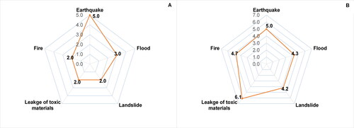
According to the triggered relationship between hazards (see Figure 2), the initial intensity degree of each hazard is adjusted before the multi-hazard intensity calculation. The adjustment principle is shown in Table 1. Using Figure 3 as an example, since earthquakes, landslides and floods all have a certain probability of inducing fires, and the intensity degree of these three hazards are 5, 2 and 3, respectively. The intensity of fire is adjusted from 2 to 4.7 (1.5 × 1.3 × 1.2 × 2). Correspondingly, the intensity degrees of earthquake, landslide and flood are also adjusted as 5, 4.2, 4.3 and 6.1, respectively. The adjusted intensity degree is shown by the radar graph in Figure 3(b). Compared to the initial radar graph, the adjusted radar graph highlights the danger degree of secondary disasters (such as fires), and it can better reflect the actual disaster situation. In the hazard identification and analysis section, the initial intensity degrees of all hazards are unified to the same classification standard (0–5), and the adjusted hazard intensity degrees are also on the same classification standard. Therefore, the final multi-hazard intensity can be calculated by summing up the adjusted intensity degree of every single hazard as shown in Eq. (1)(1) $$MH=\sum _{i=1}^n\mathit{Hai}\mathrm{ }$$(1) . (1) $$MH=\sum _{i=1}^n\mathit{Hai}\mathrm{ }$$(1) where, H_airepresents the adjusted intensity degree of hazard i, i = 1,2,…n; and MH represents the multi-hazard intensity.

Table 1. Adjustment principle for hazard intensity.

Primary hazard situation	Intensity degree of primary hazard	Adjustment principle
For hazard that needs adjustment, there is no primary hazard that induces its occurrence	–	Adjusted intensity degree = Initial intensity degree × 1
For hazard that needs adjustment, there is a primary hazard that has a high probability to induce its occurrence	5	Adjusted intensity degree = Initial intensity degree × 1.5
	3–4	Adjusted intensity degree = Initial intensity degree × 1.4
	1–2	Adjusted intensity degree = Initial intensity degree × 1.3
For hazard that needs adjustment, there is a primary hazard that has a low probability to induce its occurrence	5	Adjusted intensity degree = Initial intensity degree × 1.3
	3–4	Adjusted intensity degree = Initial intensity degree × 1.2
	1–2	Adjusted intensity degree = Initial intensity degree × 1.1

2.4. Multi-hazard risk mapping

In general, the risk is defined as the probability of loss caused by the interactions between the vulnerability of exposure and the hazard (Intentional Strategy for Disaster Reduction (ISDR) 2004). Hence, in this paper, multi-hazard risk is calculated as a function of multi-hazard intensity and vulnerability of exposure (Eq. (2)(2) $$\mathit{Risk}=\mathit{Hazard}\times \mathit{Vulnerabilty}$$(2) ). Briefly, vulnerability is given a relatively broad definition as the conditions dependent on physical, social, economic and environmental factors, which determine the potential extent of damage following exposure to hazard (Pelling 2003). Since the impact scope of a technological hazard is usually on the local scale, it is difficult to apply the vulnerability index based on administrative division statistics to the risk assessment of technological hazards. Therefore, in this paper, land use data is selected to characterize vulnerability. As shown in Table 2, according to the population density and building density of different land use types, the vulnerability is divided into five levels. For example, residential areas, schools and hospitals are the most densely populated, so residential, educational and medical land are classified as highly vulnerable areas. At last, multi-hazard risk map is drawn to show the calculated risk information with ArcGIS software. (2) $$\mathit{Risk}=\mathit{Hazard}\times \mathit{Vulnerabilty}$$(2)

Table 2. Classification of vulnerability degree.

Vulnerability degree (value)	Land use type
High (5)	Land for residential, education and medical care
Medium High (4)	Commercial land, industrial land
Medium (3)	Land for municipal public facilities
Medium Low (2)	Forestland, cultivated land
Low (1)	Grassland, wasteland

3. A case study in Huairou Science City, Beijing

3.1. Study area and data

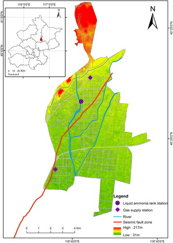
Huairou Science City (HSC), covering an area of 68.4 square kilometres, is located in the northeast of Beijing. As a key national science centre in Beijing, the region contains a large number of scientific research institutions. This region is affected by the Huangzhuang-Gaoliying seismic fault zone, and the river network is relatively dense (Figure 4). In addition, there are some industrial parks in this region, which contain liquid ammonia and other hazardous materials. Therefore, the region is threatened by multiple natural and technological disasters.

Figure 4. HSC, Beijing.

Three types of data are needed to implement the proposed methodology: natural hazard data, technological hazard data and land use data. Natural hazard data mainly includes meteorological data from meteorological stations, hydrologic data from hydrological stations and seismic data from China Earthquake Administration. Technological hazard data, collected from the local Emergency Management Bureau, includes the types and reserves of hazardous material. Land use data was derived from Landsat TM/ETM remote sensing image and modified through field research.

3.2. Hazard identification and analysis in HSC

According to the characteristics of hazard-forming environment (see Figure 4), e.g. the distributions of fault zones, river basins and hilly areas, the major natural hazards are earthquake, flood and landslide. Among these hazards, earthquake influences the entire study area. The closer to the fault zone, the greater the earthquake damage, thus the intensity of earthquake is indicated by the distance from the fault zone (Table 3 and Figure 5(a)) (Pacheco et al. 1993). Based on the historical rainfall data and hydrological data, the Hydrologic Engineering Center–River Analysis System (Brunner et al. 2016; Rawat et al. 2017) is adopted to estimate the impact scope of flood (as shown in Figure 5(b)). The inundation depth of 100-year return period rainfall is used to indicate the flood intensity (Table 3). Since soil characteristics are quite homogeneous in the study area, we only use the slope for identifying the impact scope and intensity of landslide (Table 3 and Figure 5(c)) (Guzzetti et al. 1999; Mousavi et al. 2011).

Figure 5. Intensity degree of earthquake (A), flood (B), landslide (C).

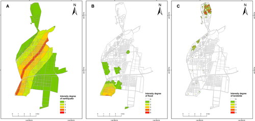
Table 3. Dividing standard for intensity degree of earthquake, flood and landslide.

Earthquake
Intensity degree	Dividing standard
5	Distance from the fault zone ≤30 m
4	30m＜Distance from the fault zone ≤200 m
3	200m＜Distance from the fault zone ≤1000 m
2	1000m＜Distance from the fault zone ≤2000 m
1	Distance from the fault zone > 2000m
Flood
Intensity degree	Dividing standard
5	Submerged depth > 3m
4	2m＜Submerged depth ≤ 3m
3	1m＜Submerged depth ≤ 2m
2	0.5m＜Submerged depth ≤ 1m
1	0m＜Submerged depth ≤ 0.5m
Landslide
Intensity degree	Dividing standard
5	Slope > 25°
4	20°＜Slope ≤ 25°
3	16°＜Slope ≤ 20°
2	12°＜Slope ≤ 16°
1	8°＜Slope ≤ 12°

In terms of technological hazards, there are three major hazard sources in the study area, i.e. two compressed natural gas supply stations (the maximum gas storage capacity of each station is 30,000 m³), and a liquid ammonia tank station (the maximum storage of liquid ammonia is 14 ton). In the case of a compressed natural gas leak, the compressed natural gas would quickly evaporate to form a vapour cloud. An explosion would occur if the vapour cloud is ignited by an open flame. Here, it is assumed that the largest reserves of natural gas would be completely released, i.e. leakage of 30,000 m³ natural gas in each compressed natural gas supply station. A vapour cloud explosion model is applied to estimate the damaging effect and damage radius of the explosion (Eq. (3)(3) $$W_{\mathit{TNT}}=1.8A{W}_{\mathit{f}}{Q}_{\mathit{f}}/Q_{\mathit{TNT}}$$(3) and (4)(4) $$R=0.396W_{\mathit{TN}{T}^{1/3}}\hspace{0.17em}\text{exp}[3.5031-0.7241\hspace{0.17em}\text{ln}\hspace{0.17em}\Delta P+0.0398{(\hspace{0.17em}\text{ln}\hspace{0.17em}\Delta P)}^2]$$(4) ) (Lenoir and Davenport 1993; Zhang et al. 2019), and the intensity of explosion is classified according to the damaging effect in Table 4. (3) $$W_{\mathit{TNT}}=1.8A{W}_{\mathit{f}}{Q}_{\mathit{f}}/Q_{\mathit{TNT}}$$(3) where, W_TNT represents the TNT equivalent of the vapour cloud (kg); A represents the efficiency factor of the vapour cloud explosion, which is 0.04; W_f is the quality of combustible gas in the vapour cloud (kg); Q_f is the combustion heat of the combustible gas (kJ/kg), which is 37,000 kJ/kg; and Q_TNT is the explosion heat of the TNT (kJ/kg), which is 4500 kJ/kg in this study. (4) $$R=0.396W_{\mathit{TN}{T}^{1/3}}\hspace{0.17em}\text{exp}[3.5031-0.7241\hspace{0.17em}\text{ln}\hspace{0.17em}\Delta P+0.0398{(\hspace{0.17em}\text{ln}\hspace{0.17em}\Delta P)}^2]$$(4) where, R is the damage radius of explosion(m); and ΔP is the overpressure (kPa).

Table 4. Dividing standard for intensity degree of explosion.

Overpressure (kPa)	Damage effect	Radius of explosion damage (m)	Intensity degree
1.035	Breaking of glass window	299.94	1
6.90	Structure damage	88.09	2
17.25	Serious casualties	54.01	3
69.0	Collapse of building	29.26	4
138.0	Death of human	22.80	5

Liquid ammonia, stored in tanks at high pressure in liquid form, evaporates into ammonia instantly after leakage. When the concentration of ammonia in the air reaches 0.5%, it would be fatal for humans to inhale for 5–10 minutes. Following previous ammonia leakage accidents (Tan et al. 2017), the release rate of leakage is set to 2.42 kg/s for 10 minutes in this study. According to the regional meteorological conditions, we set wind speed set to 0.5 m/s, 1.5 m/s, 2.9 m/s (annual average wind speed), 3.0 m/s. The atmospheric stability is set to D, E and F. Then, the Gaussian diffusion model is used to estimate the concentration distribution of the emission under different atmospheric stability and wind speed at downwind distance under the accident state (Eq. (5)(5) $$C(x,y,\mathrm{z})=\frac{Q}{2\pi {\sigma }_y{\sigma }_{z}u}\text{exp}[-\frac{y^2}{2{\sigma }_y^2}]\{\hspace{0.17em}\text{exp}[-\frac{{(z-H)}^2}{2{\sigma }_y^2}]+\hspace{0.17em}\text{exp}[-\frac{{(z+H)}^2}{2{\sigma }_z^2}\left]\mathrm{ }\right\}$$(5) ) (Ji et al. 2014; Tan et al. 2017). The estimated results are shown in Table 5. The maximum distance at each concentration (bold value in Table 5) is selected to classify the intensity of ammonia leakage. (5) $$C(x,y,\mathrm{z})=\frac{Q}{2\pi {\sigma }_y{\sigma }_{z}u}\text{exp}[-\frac{y^2}{2{\sigma }_y^2}]\{\hspace{0.17em}\text{exp}[-\frac{{(z-H)}^2}{2{\sigma }_y^2}]+\hspace{0.17em}\text{exp}[-\frac{{(z+H)}^2}{2{\sigma }_z^2}\left]\mathrm{ }\right\}$$(5) where, C(x, y, z) is the concentration (kg/s); x is the downwind distance (m); y is the transverse wind direction distance (m); z is the height above the ground level (m); Q is the release rate of leakage (kg/s); u is the average wind speed (m/s); H is the effective discharge height (m); σ_yand σ_z are the horizontal and vertical dispersion parameters, respectively.

Table 5. Dividing standard for intensity degree of liquid ammonia leakage.

Meteorological condition		Scope of influence (m)
Atmospheric stability	Wind speed (m/s)	LC50	IDLH	PC-STEL	Nasal pharyngeal stimulation	Health standards
D	0.5	78.3	154.5	274.2	390.9	452.9
	1.5	267.5	443.7	531.8	623.3	682.7
	2.9	164.3	466.3	901.9	1087.1	1192.7
	3	159.4	457.1	925.5	1118.4	1227.4
E	0.5	99.7	180.8	283.4	380.7	433.2
	1.5	–	–	–	–	–
	2.9	263.5	748.9	911.1	1014.5	1072.6
	3	255	750.9	938.6	1046	1106
F	0.5	–	–	–	–	–
	1.5	413.7	459.1	498.1	537.8	561.8
	2.9	311.5	794	908.1	989.4	1035.1
	3	301.5	810.8	936.3	1020.9	1068.1
Intensity degree		5	4	3	2	1

Note. LC50-Lethal concentration of 50%; IDLH-Immediately dangerous to life or health; PC-STEL-Permissible concentration-short term exposure limit.

3.3. Hazard interaction analysis in HSC

Based on the impact scope of every single hazard identified in the section 3.2, the overlapping areas of different hazards impact are identified using ArcGIS. According to the matrix in Figure 2, the possible hazard interaction types in the study area are analyzed. Earthquake has a high probability of inducing landslides, explosion, and liquid ammonia leakage, a low probability of inducing flood. Flood has a low probability of inducing explosion. Since the landslide area is far from the explosion and the liquid ammonia leakage area, it is unlikely for landslide to induce explosion and liquid ammonia leakage in the study area.

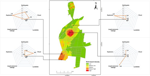
The hazard interaction analysis (Figure 6) shows that there are six hazard interaction types in the whole study area: earthquake, earthquake-flood, earthquake-landslides, earthquake-explosion, earthquake-liquid ammonia leakage and earthquake-flood-explosion. The initial radar graphs of some areas are also shown in Figure 6. Following the principle in Table 1, the radar graph is adopted to calculate the adjusted hazard intensity degree in these six types. After that, the multi-hazard intensity map is produced by synthesizing the adjusted intensity. As shown in Figure 7, the high intensity areas are mainly distributed in the core influence range of liquid ammonia leakage, and the hazard interaction type is earthquake-liquid ammonia leakage.

Figure 6. Hazard interaction types in HSC.

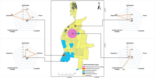
Figure 7. Multi-hazard intensity in HSC.

3.4. Multi-hazard risk mapping in HSC

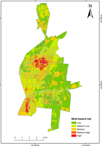
According to the density of population and buildings extracted from land use data, the vulnerability index is divided into five classes (Figure 8). The final risk is calculated by aggregating the multi-hazard intensity (Figure 7) and vulnerability index (Figure 8). The final risk map is shown in Figure 9. Our analysis shows that the high risk areas are mainly distributed in the central and southwest area. The joint action of earthquake and liquid ammonia leakage is the main reason for high risk in the central area. Thus, studying the multi-hazard risk that might be caused by the coupling of natural and technological hazards is essential for risk prevention. Furthermore, the risk in the southwest area is also high due to its dense population and combined effects of earthquakes and floods.

Figure 8. Vulnerability index in HSC.

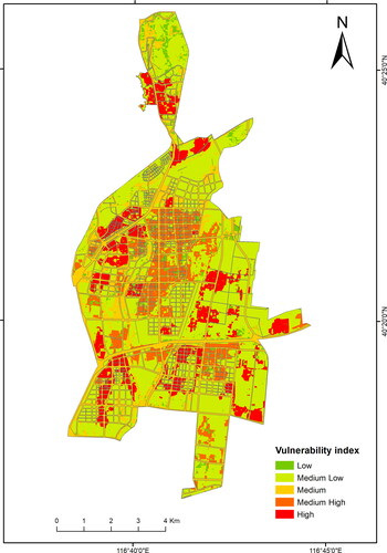
Figure 9. Multi-hazard risk map in HSC.

4. Conclusion and discussion

The new methodology developed in this study filled a key research gap in the existing multi-hazard risk mapping research. Most of the previous multi-hazard risk maps only focused on the risk induced by natural hazards and ignore technological hazards. By contrast, the new methodology calculates multi-hazard risk with an explicit consideration of coupling effect between natural and technological hazards based on hazard matrix and radar graph. In this study, the triggered relationships among natural and technological hazards were analyzed for the first time using a hazard matrix. The matrix can be adapted and scaled for application in specific locations to analyze the influence of the interaction between natural and technological hazards. Based on the triggered relationships shown in the matrix, the radar graph was adopted to adjust the intensity of each hazard in a specific area. The adjusted hazard intensity is the intensity under the coupling effect of all hazards in this area. In this way, the adjusted radar graph can display all possible hazards in this area, and also clearly show the impact of each hazard on the area under the action of hazard coupling.

In conclusion, with the help of the hazard matrix and radar graph, the methodology developed in this study helps public planners and decision-makers to better understand the possible interactions among different natural and technological hazards. This should allow them to implement appropriate and more targeted mitigation measures. Public planners and decision-makers can also use the assessment results to help residents and other organizations to better understand the natural or technological hazards they are exposed to, thus enhancing public risk awareness and informing local risk management.

Overall, this study has constructed a useful tool for analyzing the coupling effect between natural and technological hazards. Nevertheless, we still do not fully understand the interaction mechanism of natural and technological hazards. This study did not calculate the probability of natural hazards inducing technological hazards. Probability calculation usually requires a large amount of historical disaster data in the field of risk assessment, but historical data in most areas is insufficient. It would be interesting to explore a new way of addressing this issue without historical data in the future.

Data availability statement

Hydrologic data were collected from local hydrological stations in Huairou, and seismic data were collected from China Earthquake Administration. Technological hazard data were generated at Beijing Emergency Management Bureau. Landsat TM/ETM remote sensing image were obtained from Resource and Environmental Science and Data Center (https://www.resdc.cn/data.aspx?DATAID=184). Derived data supporting the findings of this study are available from the corresponding author [J.F] on request.

Disclosure statement

No potential conflict of interest was reported by the authors.

Additional information

Funding

This work was supported by the National Natural Science Foundation of China [grant number 41807510]; and Foundation of President of Institutes of Science and Development, Chinese Academy of Sciences [grant number Y9X1791Q01].

References

- Aksha SK, Resler LM, Juran L, Laurence WC. 2020. A geospatial analysis of multi-hazard risk in Dharan, Nepal. Geomatics Nat Hazards Risk. 11(1):88–111.
- Barrantes G. 2018. Multi-hazard model for developing countries. Nat Hazards. 92(2):1081–1095.
- Bathrellos GD, Skilodimou HD, Chousianitis K, Youssef AM, Pradhan B. 2017. Suitability estimation for urban development using multi-hazard assessment map. Sci Total Environ. 575:119–134.
- Brunner GW, Warner J, Wolfe B, Piper S, Marston L. 2016. HEC-RAS, River Analysis System. Applications Guide. US Army Corps of Engineers Hydrologic Engineering Center, Davis (CA).
- Buck KD, Summers JK. 2020. Application of a multi-hazard risk assessment for local planning. Geomat Nat Hazards Risk. 11(1):2058–2078.
- Chen G, Huang K, Zou M, Yang Y, Dong H. 2019. A methodology for quantitative vulnerability assessment of coupled multi-hazard in Chemical Industrial Park. J. Loss Prev. Process Ind. 58:30–41.
- Dabbeek J, Silva V. 2020. Modeling the residential building stock in the Middle East for multi-hazard risk assessment. Nat Hazards. 100(2):781–810.
- Dai FC, Lee CF, Deng JH, Tham LG. 2005. The 1786 earthquake-triggered landslide dam and subsequent dam-break flood on the Dadu River, Southwestern China. Geomorphology. 65(3–4):205–221.
- Eshrati L, Mahmoudzadeh A, Taghvaei M. 2015. Multi hazards risk assessment, a new methodology. Int J Health Syst Disaster Manage. 3(2):79–88.
- Gallina V, Torresan S, Critto A, Sperotto A, Glade T, Marcomini A. 2016. A review of multi-risk methodologies for natural hazards: consequences and challenges for a climate change impact assessment. J Environ Manage. 168:123–132.
- Gautam D, Thapa S, Pokhrel S, Lamichhane S. 2021. Local level multi-hazard zonation of Nepal. Geomatics Nat Hazards Risk. 12(1):405–423.
- Gill JC, Malamud BD. 2014. Reviewing and visualizing the interactions of natural hazards. Rev Geophys. 52(4):680–722.
- Girgin S, Necci A, Krausmann E. 2019. Dealing with cascading multi-hazard risks in national risk assessment: The case of Natech accidents. Int. J. Disaster Risk Reduct. 35:101072.
- Grünthal G, Thieken AH, Schwarz J, Radtke KS, Smolka A, Merz B. 2006. Comparative risk assessment for the city of Cologne-storms, floods, earthquake. Nat Hazards. 38(1-2):21–44.
- Guzzetti F, Carrara A, Cardinali M, Reichenbach P. 1999. Landslide hazard evaluation: a review of current techniques and their application in a multi-scale study, Central Italy. Geomorphology. 31(1–4):181–216.
- He Z, Weng W. 2020. Synergic effects in the assessment of multi-hazard coupling disasters: Fires, explosions, and toxicant leaks. J Hazard Mater. 388:121813.
- Intentional Strategy for Disaster Reduction (ISDR). 2004. Living with risk. A global review of disaster reduction initiatives. United Nations Publication, Geneva.
- Ji J, Chen X, Han X. 2014. Rapid simulation and visualization analysis of liquid ammonia tank leakage risk. Procedia Eng. 84:682–688.
- Kappes MS, Keiler M, von Elverfeldt K, Glade T. 2012. Challenges of analyzing multi-hazard risk: a review. Nat Hazards. 64(2):1925–1958.
- Komendantova N, Mrzyglocki R, Mignan A, Khazai B, Wenzel F, Patt A, Fleming K. 2014. Multi-hazard and multi-risk decision-support tools as a part of participatory risk governance: feedback from civil protection stakeholders. Int J Disaster Risk Reduct. 8:50–67.
- Lenoir EM, Davenport JA. 1993. A survey of vapour cloud explosions: Second update. Proc Safety Prog. 12(1):12–33.
- Liu B, Siu YL, Mitchell G. 2016b. Hazard interaction analysis for multi-hazard risk assessment: a systematic classification based on hazard-forming environment. Nat Hazards Earth Syst Sci. 16(2):629–642.
- Liu B, Siu YL, Mitchell G. 2017. A quantitative model for estimating risk from multiple interacting natural hazards: an application to northeast Zhejiang. Stoch Environ Res Risk Assess. 31(6):1319–1340.
- Liu B, Siu YL, Mitchell G, Xu W. 2016a. The danger of mapping risk from multiple natural hazards. Nat Hazards. 82(1):139–153.
- Marzocchi W, Garcia-Aristizabal A, Gasparini P, Mastellone M, Di Ruocco A. 2012. Basic principles of multi-risk assessment: a case study in Italy. Nat Hazards. 62(2):551–573.
- Mousavi SZ, Kavian A, Soleimani K, Mousavi SR, Shirzadi A. 2011. GIS-based spatial prediction of landslide susceptibility using logistic regression model. Geomatics Nat Hazards Risk. 2(1):33–50.
- Norio O, Ye T, Kajitani Y, Shi P, Tatano H. 2011. The 2011 eastern Japan great earthquake disaster: overview and comments. Int J Disaster Risk Sci. 2(1):34–42.
- Pacheco JF, Sykes LR, Scholz CH. 1993. Nature of seismic coupling along simple plate boundaries of the subduction type. J Geophys Res. 98(B8):14133–14159.
- Pelling M. 2003. The vulnerability of cities. Natural disasters and social resilience. Earthscan Publications, London.
- Pourghasemi HR, Gayen A, Edalat M, Zarafshar M, Tiefenbacher JP. 2020. Is multi-hazard mapping effective in assessing natural hazards and integrated watershed management? Geosci. Front. 11(4):1203–1217.
- Rawat PK, Pant CC, Bisht S. 2017. Geospatial analysis of climate change and emerging flood disaster risk in fast urbanizing Himalayan foothill landscape. Geomatics Nat Hazards Risk. 8(2):418–447.
- Satir O, Berberoglu S, Donmez C. 2016. Mapping regional forest fire probability using artificial neural network model in a Mediterranean forest ecosystem. Geomatics Nat Hazards Risk. 7(5):1645–1658.
- Schmidt-Thomé P. 2006. Natural and technological hazards and risks affecting the spatial development of European region. Geological Survey of Finland, Luxembourg.
- Sutanto SJ, Vitolo C, Napoli CD, Andrea MD, Van Lanen HAJ. 2020. Heatwaves, droughts, and fires: Exploring compound and cascading dry hazards at the pan-European scale. Environ. Int. 134:105276.
- Tan W, Du H, Liu L, Su T, Liu X. 2017. Experimental and numerical study of ammonia leakage and dispersion in a food factory. J. Loss Prev. Process Ind. 47:129–139.
- Tilloy A, Malamud BD, Winter H, Laugel AJ. 2019. A review of quantification methodologies for multi-hazard interrelationships. Earth-Sci. Rev. 196:102881.
- Xie P, Wen H, Ma C, Baise LG, Zhang J. 2018. Application and comparison of logistic regression model and neural network model in earthquake-induced landslides susceptibility mapping at mountainous region, China. Geomatics Nat Hazards Risk. 9(1):501–523.
- Zeng T, Chen G, Reniers G, Yang Y. 2021. Methodology for quantitative risk analysis of domino effects triggered by flood. Process Saf Environ. 147:866–877.
- Zhang Q, Zhou G, Hu Y, Wang S, Sun B, Yin W, Guo F. 2019. Risk evaluation and analysis of a gas tank explosion based on a vapour cloud explosion model: A case study. Eng. Fail. Anal. 101:22–35.
- Zscheischler J, Westra S, van den Hurk BJJM, Seneviratne SI, Ward PJ, Pitman A, AghaKouchak A, Bresch DN, Leonard M, Wahl T, et al. 2018. Future climate risk from compound events. Nature Clim Change. 8(6):469–477.