Investigation of the seismic response characteristics of a rock mass slope containing weak structural planes under seismic excitation based on multi-domain coupling analysis

Abstract

Because of the complexity of interactions between seismic waves and rock masses, the dynamic response of slopes has typical multi-domain characteristics. To fully consider the multi-domain characteristics of ground motion, the dynamic response of a rock slope containing weak structural planes was systematically investigated in the time domain, frequency domain, and time-frequency domain. Two-dimensional dynamic analyses were carried out on two numerical models, including the homogeneous slope- and slope-containing structural planes. The results show that slopes containing structural planes have dynamic topographic and geological amplification effects. Based on the frequency-domain analysis, the relationship between the frequency of waves and the dynamic response of slopes was further studied. The geological structure influences the high-frequency components of waves in slopes containing structural planes. The analyses of the marginal spectrum show that seismic energy is mainly concentrated in the frequency band of waves (7–10 Hz). In addition, the seismic failure mechanism of slopes containing structural planes was explored. Structural planes have an important effect on the seismic failure mode of slopes containing structural planes. Multi-domain coupling analysis can reveal the seismic response characteristics of slopes more comprehensively and provide a reference for the seismic design of rock slopes.

Keywords:

• Seismic response
• multi-domain coupling analysis
• rock slope
• structural plane
• numerical dynamic analyses

1. Introduction

The landscape of Western China is mainly mountainous, and earthquakes have induced many landslides (Zhou et al. 2017; Chen et al. 2020; Chen and Song 2021). Field investigations after the 2008 Wenchuan earthquake show that seismic wave propagation in rock-soil bodies weakens the stability of slopes to a large extent (Yin et al. 2015). The spatial distribution of earthquake-induced landslides after the earthquake also reveals that seismic landslides have specific topographic and geological amplification effects (Wang et al. 2010; Huang et al. 2012). The influence of earthquakes on the stability of landslides has attracted the attention of many scholars for several years (Chen and Wu 2018; Chen, Song, Dong 2021; Chen, Song, Juliev, et al. 2021).

With long-term geological action, there are many discontinuous joints in the rock mass, including penetrating structural planes that cut the rock mass into discontinuous bodies (Wu et al. 2014; Du et al. 2020; Guo and Cui 2020; Cao et al. 2021). The discontinuous geological structure in the rock mass weakens its strength and stability (Liu et al. 2020; Song, Liu, Chen, et al. 2021). The failure modes of toppling slopes containing discontinuities mainly include bend toppling, block toppling, and massive bending and toppling (Alejano et al. 2010; Amini et al. 2012). The dynamic failure modes of rock slopes are affected by discontinuity distributions (Zhou et al. 2017; Song, Chen, et al. 2021). Due to the randomness of earthquakes and the complexity of rock mass structural materials, the stability of rock slopes is difficult to fully understand. Hence, the dynamic stability of rock slopes needs to be further studied.

Many scholars have studied the seismic dynamic response characteristics of rock slopes (Liu et al. 2013; Song, Liu, Huang, Zhang, Zhang, et al. 2021, Song, Liu, Li, et al. 2021). Time-domain analysis is the common method used to investigate the dynamic response of slopes (Fan et al. 2017; Li et al. 2018). The dynamic acceleration response is used to study the seismic response characteristics of various types of slopes, such as jointed slopes (Li et al. 2018), rock slopes with weak structural surfaces (Song, Chen, et al. 2021), and layered slopes (Fan et al. 2016). In addition, frequency-domain analysis can explore the relationships between seismic wave frequency, natural frequency, and the dynamic response characteristics of slopes (Song, Liu, Li, et al. 2021). Moore et al. (2011) investigated the dynamic response of slopes using the Fourier spectrum response of large rock slopes. Li et al. (2019) investigated the dynamic response of jointed slopes and the damage characteristics of slopes by analysing the Fourier spectrum. He et al. (2020) investigated the seismic stability of a landslide by analysing the Fourier spectrum response of a strong earthquake seismograph array. The slope instability caused by the resonance between the high frequency of waves and the natural frequency of slopes has always been a hot issue in the field of seismic engineering. Yang et al. (2015) used the Hilbert-Huang transform (HHT) to study the dynamic response of a rock landslide and its triggering mechanism from an energy perspective, which showed that time-frequency domain analysis could better reflect the dynamic response of slopes. Fan et al. (2016, 2017, 2019) used the HHT marginal spectrum to study the seismic failure mode of slopes with structural planes, suggesting that the marginal spectrum could better reflect the seismic failure development process in slopes. The dynamic response of rock slopes with complex geological structures has typical multi-domain characteristics. Time domain, frequency domain, and time-frequency domain analyses have become important methods for analysing the seismic response of slopes.

Seismic waves are typical random waves containing complex frequency components (Song, Liu, Huang, et al. 2021). Due to the heterogeneity and nonlinearity characteristics of rock masses, the seismic response characteristics of rock masses are difficult to systematically understand. The dynamic characteristics of slopes should be further clarified from the perspective of the frequency domain. Moreover, due to the time-frequency-amplitude characteristics of seismic waves, it is necessary to further reveal the seismic response of slopes in the time-frequency domain. However, previous research focussed on the time-domain analysis of the seismic response of rock slopes but ignored the frequency domain and time-frequency domain characteristics. Therefore, to solve the above problems, it is necessary to establish a multi-domain coupling analysis method to systematically reveal the seismic response characteristics of complex rock slopes considering the three domains.

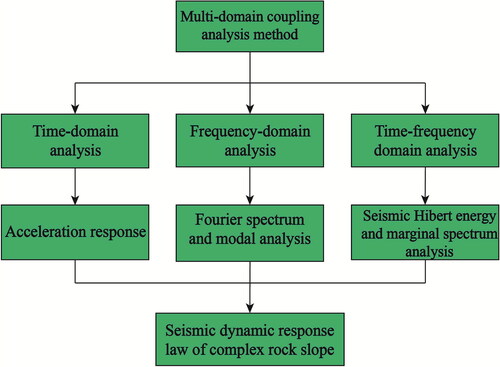
A multi-domain coupling analysis method is proposed to investigate the seismic response characteristics of a rock mass slope containing weak structural planes, as shown in Figure 1. Two-dimensional dynamic analyses are performed on two numerical models using FLAC 3 D (Fast Lagrangian Analysis of Continua). This work focuses on three aspects in this research: dynamic acceleration response (time-domain analysis), modal analysis and Fourier spectrum analysis (frequency-domain analysis), and marginal spectral analysis of the models (time-frequency domain analysis). The influence of topographic and geological conditions on the seismic response of the models was analysed. In addition, this work analyses the relationship between the natural frequencies and the dynamic characteristics of slopes. The dynamic failure mechanism of a slope containing structural planes is discussed as well.

Figure 1. Flowchart for the multi-domain coupling analysis method.

2. Numerical model and dynamic analyses

2.1. Case study

The rock slope is located in the hilly region of Sichuan Province in Western China, where the river system, gullies, and valleys are developed. The landform in the region is dominated by mountains, hills, and valley plains (Figure 2). The strata in the slope area are continuous, with gentle occurrence and no faults passing through. Under the influence of regional tectonic stress, deadweight stress, and unloading, rock joints in the area are very well developed. Several seismic fault zones are distributed near the slope. The slope body with weak structural planes is approximately 34 m long and 40 m high, with a gradient of approximately 70°. The development of the slope has multilayer weak structural planes, joints, and fissures. Weak structural planes are developed on the contact surface between silty mudstone layers. The structural planes are distributed in a zonally continuous manner on the slope. To obtain the physical and mechanical parameters of the rock mass in the slope, a series of laboratory tests, such as direct shear tests, triaxial tests, compression tests, and tensile tests, were performed (Table 1). According to the geological structure type of the slopes, the geological model of the slope is simplified, as shown in Figure 3.

Figure 2. Location of the study area.

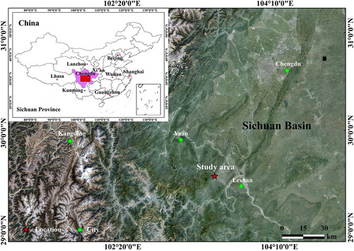
Figure 3. Boundary condition setting and layout of the monitoring points in the models: (a) homogeneous slope (Model 1); (b) toppling slope (Model 2).

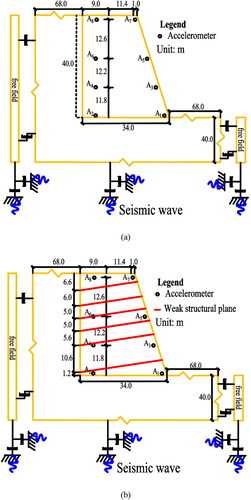
Table 1. Physico-mechanical parameters of the material parameters of the slope.

Material parameters	Density ρ (kN/m^3)	Poisson ratio μ	Elastic modulus E (MPa)	Friction angle φ (°)	Cohesive Force c (kPa)
Rock mass	2400	0.16	375	35	1200
Structural surface	18.4	0.35	35	23	14

2.2. Numerical model

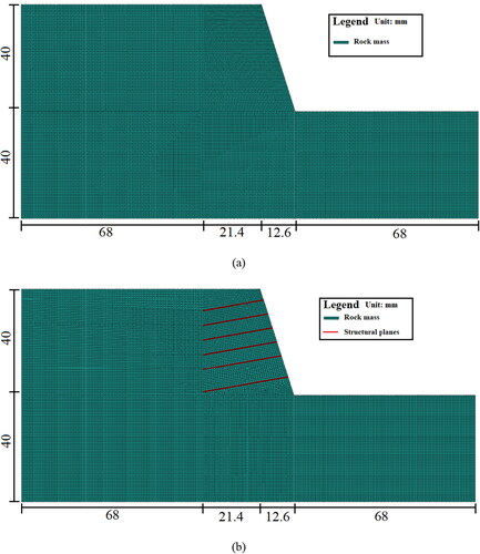
The rock mass of the model is elastoplastic material, and the Mohr-Coulomb strength criterion is adopted. The calculated boundaries of the model are as follows: the length from the foot of the slope to the right boundary is twice the length of the slope, the length from the top of the slope to the left boundary is twice the height of the slope, and the height from the top to the bottom of the slope is twice the height of the slope. The boundary range meets the requirements of calculation accuracy under static and dynamic conditions (Xu et al. 2008). Model 1 (homogeneous slope) and Model 2 (slope containing weak structural planes) were established, and the two numerical mesh models, with dimensions of 80 × 170 m, are shown in Figure 4. To reduce the difficulty of simulation, the structural planes were simplified into a weak band with a depth of 0.2 m. A quadrilateral grid with a side length of 0.5 m was used to investigate the characteristics of the model. FLAC 3 D was used as a solver for dynamic analysis via its transient dynamics simulation capability. Local damping is used in the model. In dynamic analysis, model boundary processing is a key technology. An improper boundary leads to wave reflection and refraction, which seriously affect the results of dynamic analysis. In this model, the discontinuity is simulated as a soft material rigidly connected with the rock mass, and the selection of the thickness of the discontinuity is more critical. The range of the discontinuity should be greater than the wavelength, and the thickness should be less than the wavelength.

Figure 4. Mesh model of the rock mass slopes: (a) homogeneous slope (Model 1); (b) toppling slope (Model 2).

For the dynamic response analysis of a semi-infinite space body such as a slope, the boundary problem that tends to infinity must be dealt with. FLAC provides a static boundary (viscous boundary) and free field boundary in the numerical simulation calculation. The research object in this work is a rock slope whose foundation modulus is large and can be considered a rigid foundation. Therefore, static boundary conditions are not required at the bottom of the model. The free field boundary is set around the model so that the side boundary of the main grid is coupled with the free field grid through dampers. The unbalanced force of the free field grid is applied to the boundary of the main grid. The boundary conditions are set as shown in Figure 3b. To study the dynamic response of the slope, some monitoring points are set up in the model. To eliminate the adverse effect of the deadweight of the slope, a stress balance should be carried out before the numerical simulation.

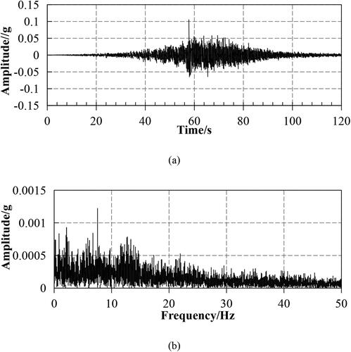
Two loading directions of Wenchuan earthquake waves (the z and x directions) were applied at the bottom boundary of the model, and the corresponding time history curve and Fourier spectrum are shown in Figure 5. The Wenchuan earthquake (WE) waves were recorded at Wudu in Gansu, China. The dominant frequency wave is 7.74 Hz, t = 120 sec, and Δt = 0.005 sec to create time-dependent acceleration inputs at the bottom of the slope during horizontal and vertical motions in the dynamic calculations.

Figure 5. The input WE wave (0.1 g): (a) Time history; (b) Fourier spectrum.

3. Multi-domain coupling analysis of the dynamic response characteristics of slopes

3.1. Analysis of the time domain

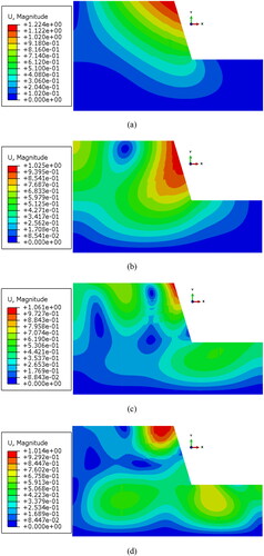
To analyse the influence of structural planes on the wave propagation characteristics, taking the input wave (0.1 g) as an example, the acceleration distribution of the models at different times was extracted. The acceleration distributions of the two models are shown in Figures 6-9. Waves mainly propagate along the slope surface from the bottom to the slope crest. Comparing Model 1 and Model 2 reveals that the acceleration distribution characteristics of Model 2 have apparent changes. A noticeable change in the phase difference can be found on both sides of the weak planes. Furthermore, the local magnification amplification effect of the toppling slope can be identified, which indicates that structural planes affected the propagation characteristics of waves inside the slope. This effect occurs because the existence of structural planes causes refraction and reflection effects of waves when waves propagate in the rock mass so that waves appear superposed near weak planes, further resulting in a local amplification effect of waves.

Figure 6. Wave propagation characteristics through the Model 1 when the WE wave is input in the x-direction (unit: m/s²): (a) t = 0.02 s; (b) t = 0.03 s; (c) t = 0.04 s; (d) t = 0.05 s.

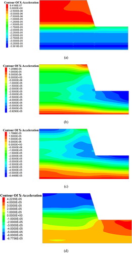
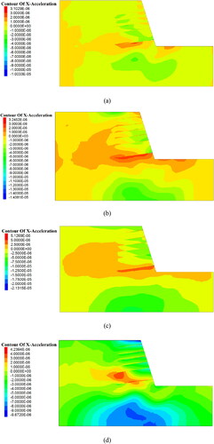
Figure 7. Wave propagation characteristics through the Model 2 when the WE wave is input in the x-direction (unit: m/s²): (a) t = 0.02 s; (b) t = 0.03 s; (c) t = 0.04 s; (d) t = 0.05 s.

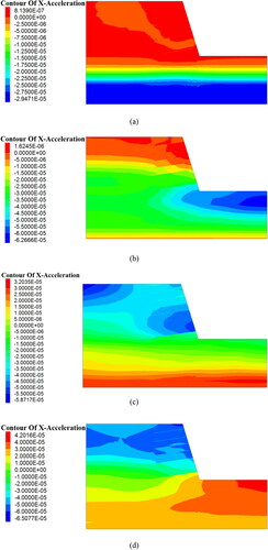
Figure 8. Wave propagation characteristics through the Model 1 when the WE wave is input in the z-direction (unit: m/s²): (a) t = 0.02 s; (b) t = 0.03 s; (c) t = 0.04 s; (d) t = 0.05 s.

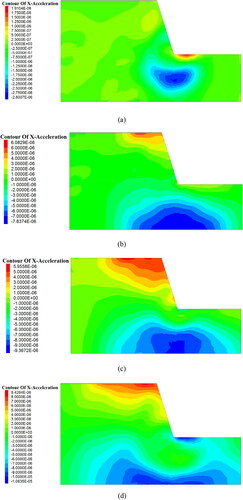
Figure 9. Wave propagation characteristics through the Model 2 when the WE wave is input in the z-direction (unit: m/s²): (a) t = 0.02 s; (b) t = 0.03 s; (c) t = 0.04 s; (d) t = 0.05 s.

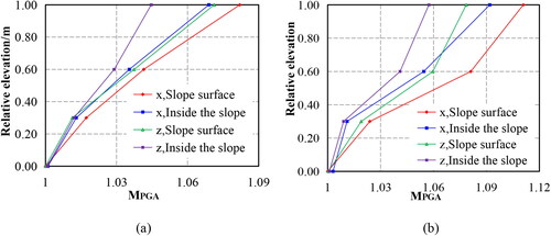
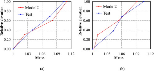
The peak ground acceleration (PGA) reflects the strongest response in the whole acceleration time history and reflects the maximum seismic inertial force at a certain position in the slope body. The M_PGA is used to analyse the acceleration response of slopes. The ratio of PGA at any point on the slope to PGA at the foot of the slope (A1 point) was defined as M_PGA, which represents acceleration magnification at a point of the slope. Four typical monitoring points (A1, A3, A15, and A7) of the slope surface are selected, and their acceleration-time histories and Fourier spectra curves are shown in Figures 10 and 11. The changes in M_PGA with relative elevation (h/H) are shown in Figure 12. h/H refers to the ratio of the height of one point to the height (H) of slopes. h refers to the height from the bottom of slopes. Figure 12a shows that the M_PGA of Model 1 increases with elevation and reaches the maximum at the slope crest. The M_PGAmax values are approximately 1.2 and 1.14 when the input waves are in the x- and z-directions, respectively. This shows that the acceleration amplification effect of the slope increases with elevation, and the slope has a dynamic elevation amplification effect. The M_PGA of Model 2 increases with elevation as well, indicating that the slope also has a typical elevation dynamic amplification effect (Figure 12b). However, comparing Figure. 12a and b, the M_PGA of Model 1 shows an increasing linear trend with elevation overall, while Model 2 shows a significant nonlinear increase, indicating that the structural planes influence the dynamic magnification effect of the model. This effect occurs because structural planes cause the discontinuity of the rock mass, and the refraction and reflection effects of waves appear near the weak structural plane, which leads to the nonlinear variation characteristics of the amplification effect. The M_PGA at the slope surface is significantly larger than that inside the slope, suggesting that the slope has a significant amplification effect on the slope surface. Moreover, the M_PGA of Model 2 is approximately 1.1 times that of Model 1, which suggests that the structural plane has a specific amplification effect on the slope. In addition, in Model 1 (Figure 12a), the M_PGAmax under horizontal seismic force is approximately 1.05 times that under vertical seismic force. In Model 2 (Figure 12b), the M_PGAmax under horizontal seismic force is approximately 1.15 times that under vertical seismic force. This finding indicates that the directions of seismic excitation influence the dynamic response of the slopes, and the acceleration amplification effect under horizontal earthquake excitation is greater.

Figure 10. Acceleration time history and Fourier spectrum of the measuring points at the slope surface (Model 1): (a) Acceleration-time histories; (b) Fourier spectrum.

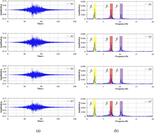
Figure 11. Acceleration time history and Fourier spectrum of the measuring points at the slope surface (Model 2): (a) Acceleration-time histories; (b) Fourier spectrum.

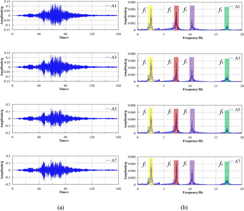
Figure 12. M_PGA change rule of the slope when inputting the WE wave (0.1 g): (a) Model 1; (b) Model 2.

Fan et al. (2016) carried out a laboratory shaking table scaled model test on Model 2, and the comparison between the model test and the numerical test results is shown in Figure 13. The acceleration amplification factor obtained from the model test is similar to the numerical simulation result, indicating that the numerical result is reliable. In the numerical model, the size and physico-mechanical parameters of the model are the same as those of the original slope. However, in the laboratory model test, the physico-mechanical parameters of the model are calculated according to the similarity ratio. The experimental model is a scaled model with a certain size effect compared to the original slope. During the construction of the test model, there are some differences in the adhesion between the simulated rock mass and the structural plane, which is different from the original slope. These factors directly lead to the difference between the numerical results and the model test results. However, in general, the numerical results and experimental results can better reflect the dynamic response patterns of the slope, and the results of both analyses confirm each other.

Figure 13. M_PGA change rule of the toppling slope when the WE wave is input in the x direction (0.1 g): (a) inside the slope; (b) near the slope surface.

3.2. Analysis of the frequency-time domain

The frequency-domain analysis mainly includes modal analysis and Fourier spectrum analysis. The principles of FFT and modal analysis are as follows. Modal analysis has become widely used type of dynamic frequency-domain analysis (Reale et al. 2016; Song, Liu, Li, et al. 2021). Modal analysis can reveal slopes' natural frequency and vibration mode and predict the dynamic response of slopes in the elastic domain. It is worth noting that the low-order vibration mode has a controlling effect on the dynamic characteristics of the engineering body. Therefore, in modal analysis, only the first few modes are considered. In addition, FFT is used to analyse the vibration response of rock and soil masses, which can identify different frequency components of signals. FFT can quickly identify the main components of the signal and can also be quickly filtered, which has become a common method to deal with seismic wave signals.

The modal analysis results of the models are shown in Figures 14–16. Figure 14 shows that the natural frequencies (f) of the slopes increase with the order. The first four f values of Model 1 are 2.96, 7.84, 11.18, and 18.06 Hz, respectively. The corresponding f values of Model 2 are 2.81, 7.34, 10.69, and 17.63 Hz, respectively. The natural frequency of Model 2 is less than that of Model 1 because Model 2 contains multiple structural planes, which decreases the stiffness of the rock mass. This finding suggests that structural planes affect the natural frequency of the models. In Figures 15 and 16, U refers to the relative displacement of the models under a certain mode of vibration. Figures 15 and 16 show that the first four modes of Model 1 are similar to Model 2 overall. However, U near the structural planes of Model 2 has a discontinuous distribution, with a certain phase shift, which indicates that the structural plane affects the dynamic response of the rock mass. Figures 15 and 16 show that the U_max of Model 2 is larger than that of Model 1; in particular, the higher-order modal characteristics of the slopes are different. This difference arises because structural surfaces enlarge the slope deformation. The modal characteristics of different orders show that the U of the slope increases with the slope height, on the whole, suggesting that the slopes have a pronounced elevation amplification effect and are prone to damage on the slope crest. Moreover, Figures 15 and 16 also show that under the same elevation condition, the U of the slope surface is significantly larger than that inside the slope body, which is similar to the time-domain results.

Figure 14. Natural frequency of the slope according to modal analysis by using FEM.

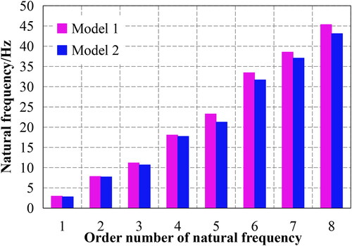
Figure 15. Results of modal analysis of the homogeneous slope: (a) Mode 1 (2.96 Hz); (b) Mode 2 (7.84 Hz); (c) Mode 3 (11.18 Hz); (d) Mode 4 (18.06 Hz).

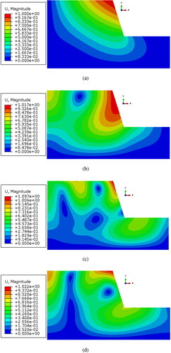
Figure 16. Results of modal analysis of the toppling slope: (a) Mode 1 (2.81 Hz); (b) Mode 2 (7.34 Hz); (c) Mode 3 (10.69 Hz); (d) Mode 4 (17.63 Hz).

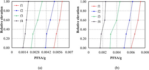
In addition, the dynamic response of the slope is further analysed by using Fourier spectrum analysis. Figures 10 and 11 shows that Model 1 comprises three predominant frequencies (f₁-f₃), and Model 2 has four predominant frequencies (f₁-f₄). The values of the predominant frequencies are similar to those in the modal analysis. Fourier spectrum analysis and modal analysis further determined the f of the slopes. It is worth noting that Model 2 has f₄, which indicates that structural planes have a noticeable magnification effect on the high-frequency components of waves. Figures 17 and 18 show that the PFSA of the slopes increases with elevation at different natural frequencies. Compared with the PFSA of the internal slope body, the slope surface is significantly larger. This indicates that the slope has prominent elevation and slope surface magnification effects, consistent with the analysis results in the time domain. Moreover, the PFSA of Model 2 is approximately 1.3 times that of Model 1. The PFSA of f₁ and f₂ shows an increasing linear trend, while that of f₃ and f₄ shows a nonlinear increasing trend overall, suggesting that the structural plane affects the high-frequency components of waves. Therefore, modal analysis and Fourier spectrum analysis can identify the relationship between the frequency components of waves and the amplification effect of slopes.

Figure 17. The PFSA change rule of the homogeneous slope when inputting the WE wave in the x direction: (a) at the slope surface; (b) inside the slope.

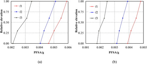
Figure 18. The PFSA change rule of the toppling slope when inputting the WE wave in the x direction: (a) at the slope surface; (b) inside the slope.

3.3. Analysis of the time-frequency domain

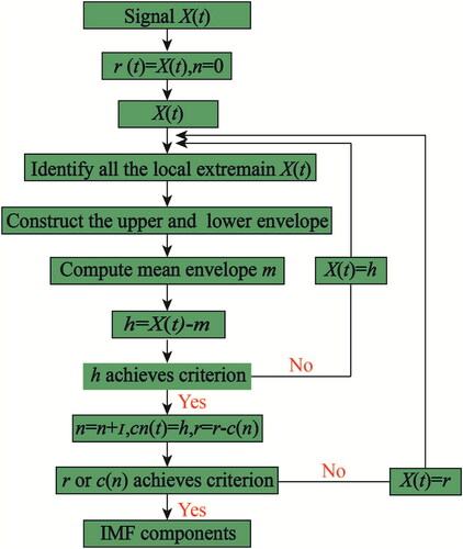
The HHT method is mainly composed of the empirical mode decomposition (EMD) method and Hilbert spectrum analysis (HSA), which provides a feasible tool for identifying earthquake Hilbert energy distributions (Huang et al. 1998; Fan et al. 2017). Using the EMD, the seismic wave is decomposed into a series of intrinsic mode functions (IMFs). The flowchart for the EMD approach is shown in Figure 19 (Zhang 2006). The HHT marginal spectrum is defined as the integral of the Hilbert Huang spectrum on the time axis as follows: $h(\omega )={\displaystyle {\int }_0^{T}H(\omega ,t)}dt.$ The marginal spectrum can show the accumulation of IMF amplitude in the whole period. Every instantaneous frequency has a certain amount of energy. By accumulating the energy of these instantaneous frequencies, the total energy corresponding to the frequency in the original signal can be calculated, that is, the marginal spectrum amplitude (MSA). The marginal spectrum can be used to measure the contribution of each frequency value to the total Hilbert energy and corresponds to the Hilbert energy density at a certain frequency. The Hilbert marginal spectrum obtained by the HHT represents the distribution of the seismic signal energy amplitude along the frequency axis.

Figure 19. Flowchart for EMD approach (Zhang 2006).

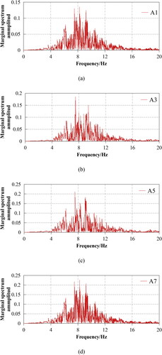
The marginal spectrum shows the energy distribution of the slope vibration, and the instantaneous spectrum can reflect the time-varying characteristics of the seismic wave signal. The propagation characteristics of seismic energy can be determined by analysing the variation in marginal spectral amplitude. Taking the acceleration time history of point A1 in Model 2 as an example, the first four IMFs and instantaneous frequency are obtained by EMD, as shown in Figures 20 and 21. Then, the marginal spectrum of the IMFs can be obtained by using HHT. As shown in Figures 20 and 21, the amplitude of IMF2 is larger, and its frequency component is much richer, which makes it easier to identify. Hence, IMF2 was used to obtain the marginal spectrum. The marginal spectrum of typical measurement points in Model 2 is shown in Figure 22. The peak marginal spectrum amplitude (PMSA) is mainly located in the range of 7–10 Hz. This frequency band is similar to f₂ and f₃ of Model 2, so the seismic wave energy in this frequency band is more suitable for analysing the dynamic response characteristics of the slope.

Figure 20. IMFs of the acceleration time history of point A1 after using the EMD when inputting the WE wave (0.1 g): (a) IMF1, (b) IMF2, (c) IMF3 and (d) IMF4.

Figure 21. Instantaneous frequencies of the acceleration time history of point A1 after using the EMD when inputting the WE wave (0.1 g): (a) Instantaneous frequency 1, (b) Instantaneous frequency 2, (c) Instantaneous frequency 3; (d) Instantaneous frequency 4.

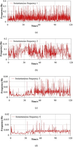
Figure 22. The marginal spectrum amplitude of the measuring points near the slope surface of Model 2 when the WE wave is input in the x direction (0.1 g): (a) A1; (b) A3; (c) A5; (d) A7.

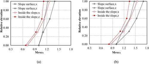
The PMSAs of the models with elevation are shown in Figure 23. The PMSA of the slopes increases with elevation, and the PMSA of the slope surface is larger than that of the internal slope. This phenomenon indicates that the slope surface and elevation magnify the energy propagation of seismic waves to a certain degree. Moreover, Figure 23 shows that the PMSAz when the input wave in the z-direction is significantly less than the PMSAx under horizontal seismic loading. The PMSAx is approximately 1.1 times that of PMSAz in Model 1, and the PMSAx of Model 2 is approximately 1.15 times that of PMSAz. This indicates that the direction of the input wave influences the energy propagation of seismic waves and the geological amplification effect when the input wave in the x-direction is larger. The PMSA of Model 2 is approximately 1.2 times that of Model 1. This difference shows that the structural plane magnifies the propagation energy of seismic waves in the rock mass. Therefore, the dynamic response of slopes can be investigated from an energy-based perspective in the time-frequency domain.

Figure 23. The change rule of PMSA with elevation of the slopes when inputting the WE wave: (a) Model 1; (b) Model 2.

4. Dynamic deformation characteristics of the slope

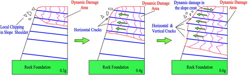
The dynamic deformation characteristics and evolution process of the slope can be investigated by analysing the distribution of shear strain increments of the slope under earthquakes. The contour of the shear strain increment of the slope under different ground motion intensities is shown in Figure 24. Figure 24 shows that the maximum value of the shear strain increment appears in the weak structural planes, while the value of the shear strain increment in the rock of the slope body is small, which indicates that weak structural planes are the most prone to shear failure subject to earthquake excitation; that is, the structural planes are the potential slip planes of the slope. Figure 24 shows that at the initial stage of ground motion, the shear strain increment of the topmost structural surface is large under small earthquakes (Figure 24a, b), which indicates that the top of the slope is the area most prone to damage. With the increase in ground motion, the increment of shear strain gradually transfers to the lower part of the slope body (Figure 24c, d), which indicates that the sliding surface gradually expands to the bottom of the slope as the shear strain in the sliding range of the slope continues to expand with the increase in ground motion. These results of the damage process of the slope are consistent with the results of the shaking table test (Figure 25) (Fan et al. 2016). Therefore, the structural planes greatly impact the failure mode of the slope, which are the potential sliding planes.

Figure 24. Contours of shear strain increment in the weak zone when the WE wave is input in the x direction: (a) 0.1 g; (b) 0.3 g; (c) 0.4 g; (d) 0.6 g.

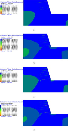
Figure 25. Failure process of the slope containing structural planes during shaking table tests (Fan et al. 2016).

5. Conclusions

A numerical dynamic analysis method is used to study the dynamic response of the two models using the multi-domain coupling analysis method. Time-domain analysis can directly and preliminarily reflect the dynamic response characteristics of slopes. Frequency-domain analysis can clarify the relationship between the wave frequency component and slope dynamic response. Time-frequency analysis can reveal the dynamic response of slopes from an energy-based perspective. The following conclusions can be drawn.

1. The results of the time-frequency joint analysis show that Model 2 has a noticeable topographic and geological dynamic amplification effect. Structural planes have an impact on the wave propagation characteristics and amplification effect of the slope. The amplification effect of the slope is increased due to the distribution of structural planes. The M_PGA, PFSA and PMSA of Model 2 are approximately 1.1, 1.3 and 1.2 times those of Model 1, respectively. Wave propagation directions have an impact on the dynamic response of the slope. The M_PGAmax under horizontal seismic loading is approximately 1.15 times that under vertical seismic loading.

2. According to the frequency-domain analysis, the natural frequency impacts the dynamic response of the slope by using the Fourier spectrum and modal analysis. Structural planes have impacts on the dynamic deformation characteristics of the slope, which have an amplification effect on the high-frequency components of waves. The natural frequencies of Model 2 are smaller than those of Model 1.

3. According to the time-frequency joint analysis, in combination with the contour of the shear strain increment of Model 2, weak structural planes are potential slip surfaces and greatly affect the seismic mode of Model 2. The upper slope body is prone to deformation under small earthquakes. With the increase in earthquakes, the range of sliding bodies gradually extends to the lower slope.

However, the energy method proposed in this work has some limitations in analysing the seismic response characteristics of rock slopes with discontinuities. The marginal spectrum is obtained based on a specific order of IMF without considering the distribution of seismic Hilbert energy in the time domain; hence, it is difficult to determine the specific time when the slope is damaged. Further research can apply the energy method to the evaluation of seismic dynamic response characteristics and failure evolution process of rock slopes with complex geological structures.

Disclosure statement

The authors declare that they have no conflicts of interest.

Data availability statement

Data supporting the results of this study may be obtained at the request of the appropriate authors.

Additional information

Funding

This study was funded by the National Natural Science Foundation of China (41941019 and 52109125), the National Postdoctoral Program for Innovative Talent of China (BX20200191), the China Postdoctoral Science Foundation (2020M680583), and the Shuimu Tsinghua Scholar Program (2019SM058).

References

- Ahmed N, Rao KR. Fast Fourier transform. In: Orthogonal transforms for digital signal processing. Berlin, Heidelberg: Springer.
- Alejano LR, Gómez-Márquez I, Martínez-Alegría R. 2010. Analysis of a complex toppling-circular slope failure. Eng Geol. 114(1-2):93–104.
- Amini M, Majdi A, Veshadi MA. 2012. Stability analysis of rock slopes against block-flexure toppling failure. Rock Mech Rock Eng. 45(4):519–532.
- Cao B, Wang S, Song D, Du H, Guo W. 2021. Investigation on the deformation law of inner waste dump slope in an open-pit coal mine: A case study in southeast Inner Mongolia of China. Adv Civ Eng. 2021:1–18.
- Chen Z, Song D. 2021. Numerical investigation of the recent Chenhecun landslide (Gansu, China) using the discrete element method. Nat Hazards. (1)105 :717–733.
- Chen Z, Song D, Dong L. 2021. Characteristics and emergency mitigation of the 2018 laochang landslide in tianquan county, sichuan province, china. Sci Rep. (1)11:1578.
- Chen Z, Song D, Hu C, Ke Y. 2020. The September 16, 2017, Linjiabang landslide in Wanyuan County, China: preliminary investigation and emergency mitigation. Landslides. (1)17:191–204.
- Chen Z, Song D, Juliev M, Pourghasemi HR. 2021. Landslide susceptibility mapping using statistical bivariate models and their hybrid with normalized spatial-correlated scale index and weighted calibrated landslide potential model. Environ Earth Sci. (8)80:324.
- Chen KT, Wu JH. 2018. Simulating the failure process of the Xinmo landslide using discontinuous deformation analysis. Eng Geol. 239:269–281.
- Du H, Song D, Chen Z, Shu H, Guo ZZ. 2020. Prediction model oriented for landslide displacement with step-like curve by applying ensemble empirical mode decomposition and the PSO-ELM method. J Clean Prod. 270:122248.
- Fan G, Zhang J, Wu J, Yan K. 2016. Dynamic response and dynamic failure mode of a weak intercalated rock slope using a shaking table. Rock Mech Rock Eng. (8)49:3243–3256.
- Fan G, Zhang LM, Zhang JJ, Ouyang F. 2017. Energy-Based analysis of mechanisms of earthquake-induced landslide using hilbert-huang transform and marginal spectrum. Rock Mech Rock Eng. (9)50:2425–2441.
- Fan G, Zhang L, Zhang J, Yang C. 2019. Analysis of seismic stability of an obsequent rock slope using time-frequency method. Rock Mech Rock Eng. (10)52:3809–3823.
- Guo C, Cui Y. 2020. Pore structure characteristics of debris flow source material in the Wenchuan earthquake area. Eng Geol. 267:105499.
- He J, Qi S, Wang Y, Saroglou C. 2020. Seismic response of the Lengzhuguan slope caused by topographic and geological effects. Eng Geol. 265:105431.
- Huang MW, Chen CY, Wu TH, Chang CL, Liu SY, Kao CY. 2012. GIS-based evaluation on the fault motion-induced coseismic landslides. J Mt Sci. (5)9:601–612.
- Huang NE, Shen Z, Long SR, Wu MC, Shih HH, Zheng Q, Yen NC, Tung CC, Liu HH. 1998. The empirical mode decomposition and the Hilbert spectrum for nonlinear and non-stationary time series analysis. Proc R Soc Lond A. (1971)454:903–995.
- Li LQ, Ju NP, Zhang S, Deng XX, Sheng D. 2019. Seismic wave propagation characteristic and its effects on the failure of steep jointed toppling rock slope. Landslides. 16(1):105–123.
- Li HH, Lin CH, Zu W, Chen CC, Weng MC. 2018. Dynamic response of a dip slope with multi-slip planes revealed by shaking table tests. Landslides. (9)15:1731–1743.
- Liu GW, Song DQ, Chen Z, Yang JW. 2020. Dynamic response characteristics and failure mechanisms of coal slopes with weak intercalated layers under blasting loads. Adv Civ Eng. 2020:1–18.
- Liu H, Xu Q, Li Y, Fan X. 2013. Response of high‐strength rock slope to seismic waves in a shaking table test. Bull Seismol Soc Am. 103(6):3012–3025.
- Moore JR, Gischig V, Burjanek J, Loew S, Fah D. 2011. Site effects in unstable rock slopes: dynamic behavior of the Randa instability (Switzerland). B Seismol Soc Am. 101(6):3110–3116.
- Reale C, Gavin K, Prendergast LJ, Xue J. 2016. Multi-modal reliability analysis of slope stability. Transp Res Procedia. 14:2468–2476.
- Song D, Chen Z, Dong L, Zhu W. 2021. Numerical investigation on dynamic response characteristics and deformation mechanism of a bedded rock mass slope subject to earthquake excitation. Appl Sci. (15) 2021. 11:7068.
- Song D, Liu X, Chen Z, Chen J, Cai J. 2021. Influence of Tunnel excavation on the stability of a bedded rock slope: a case study on the mountainous area in Southern Anhui, China. KSCE J Civ Eng. (1)25:114–123.
- Song D, Liu X, Huang J, Zhang JM. 2021. Energy-based analysis of seismic failure mechanism of a rock slope with discontinuities using Hilbert-Huang transform and marginal spectrum in the time-frequency domain. Landslides. (1)18:105–123.
- Song D, Liu X, Huang J, Zhang Y, Zhang J, Nkwenti BN. 2021. Seismic cumulative failure effects on a reservoir bank slope with a complex geological structure considering plastic deformation characteristics using shaking table tests. Eng Geol. 286:106085.
- Song D, Liu X, Li B, Zhang J, Bastos JJV. 2021. Assessing the influence of a rapid water drawdown on the seismic response characteristics of a reservoir rock slope using time–frequency analysis. Acta Geotech. (4)16:1281–1302.
- Wang X, Nie G, Wang D. 2010. Relationships between ground motion parameters and landslides induced by Wenchuan earthquake. Earthq Sci. (3)23:233–242.
- Wu W, Li JC, Zhao J. 2014. Role of filling materials in a P-wave interaction with a rock fracture. Eng. Geol. 172(8):77–84.
- Xu G, Yao L, Li Z, Gao Z. 2008. Dynamic response of slopes under earthquakes and influence of ground motion parameters. Chin J Geotech Eng. 30(6):918–923.
- Yang C, Zhang J, Bi J. 2015. Application of Hilbert-Huang Transform to the analysis of the landslides triggered by the Wenchuan earthquake. J Mt Sci. (3)12:711–720.
- Yin Y, Li B, Wang W. 2015. Dynamic analysis of the stabilized Wangjiayan landslide in the Wenchuan Ms 8.0 earthquake and aftershocks. Landslides. (3)12:537–547.
- Zhang YP. 2006. HHT analysis of blasting vibration and its application [PhD thesis]. Changsha, China: Central South University. (In Chinese).
- Zhou J, Jiao M, Xing H, Yang X, Yang Y. 2017. A reliability analysis method for rock slope controlled by weak structural surface. Geosci J. (3)21:453–467.