Insights into spatial differential characteristics of landslide susceptibility from sub-region to whole-region cased by northeast Chongqing, China

Abstract

Landslides have differential characteristics in different regions. This study explores landslide susceptibility mapping (LSM) based on different evaluation units and proposes a strategy for landslides’ differential characteristics in different sub-regions. Based on data of lithology, elevation, and historical landslides, terrain units (TUs) and slope units (SUs) were obtained. LSM was developed using the Random Forest (RF) model and Light Gradient Boosting Machine (LGBM) model. The LGBM-TUs showed the highest performance and were therefore, selected to obtain LSM. The study area was divided into four sub-regions using the geographically weighted regression (GWR) model, along with spatial differential characteristics of topography conditions. The distribution and characteristics of landslides within each sub-region were assessed using GeoDetector. The results illustrated the reliability of the LGBM-TUs model. Lithology, elevation, and average annual rainfall were the dominant factors, while the influence of other factors on the occurrence of landslides was strengthened only when these factors interacted. This study proposed a new method for LSM research to insight the spatial differential characteristics of landslides in various sub-regions. Our results provide novel insights into landslide mitigation.

Keywords:

• Landslide susceptibility mapping
• evaluation units
• Light Gradient Boosting Machine
• GeoDetector

1. Introduction

Landslides are a destructive geological hazard with severe impacts on nature, society, and the economy (Froude and Petley 2018; Huang et al. 2020b; Pham et al. 2022). Landslide susceptibility mapping (LSM) is based on the spatial distribution of landslides. Considering the influencing factors of landslides, including topography, hydrology, meteorology, and human activities, the spatial distribution of landslides and their occurrence probability can be predicted, thereby facilitating landslide control (Abbaszadeh Shahri and Maghsoudi Moud 2021; Huang et al. 2021a). LSM can facilitate landslide risk management (Huang and Zhao 2018; Nhu et al. 2020) and is therefore, an important method for mitigating landslide-associated damage (Huang et al. 2020c; Min and Yoon 2021).

The methods for improving the accuracy of LSM are primarily based on two aspects, namely, the model and evaluation units. Following the continuous development and improvement of mathematical models, condition analysis, frequency ratios, and regression analysis are used (Camilo et al. 2017; Jones et al. 2021), along with machine learning (Zhao et al. 2020, 2022; Zhou et al. 2022). Wang et al. (2020) used Random Forest (RF) algorithm and Frequency Ratio to conduct LSM on Yunyang County as the precision of the RF algorithm is better than that of other statistical algorithms. Ge et al. (2018) conducted LSM in the Longnan area of the Gansu Province and showed that the machine learning model exhibited better accuracy and stability than the statistical algorithms. To improve the accuracy of a single learning algorithm, ensemble learning, which combines multiple simple algorithms to form a model with high performance optimization, has been proposed (Zhao et al. 2021a, 2021b). Previous studies on landslides used ensemble learning to evaluate LSM and achieved higher accuracy than the single learning algorithm (Pham et al. 2017; Dou et al. 2019; Rong et al. 2020; Huang et al. 2020a). However, different ensemble learning algorithms are associated with different advantages and disadvantages (Table 1). Therefore, this study selected a typical algorithm from the Bagging and Boosting as the LSM model, where the RF model was selected for Bagging, while the Light Gradient Boosting Machine (LGBM) model was selected for Boosting. The accuracy and capability of the two models were compared. In addition, evaluation units are the basis of LSM and significantly affect its accuracy. Grid units (GUs) and slope units (SUs) are commonly used, while geomorphic units, specific condition units, and administrative units are occasionally used. SUs can express terrain features more accurately, thereby significantly improving the accuracy of results.

Table 1. Advantages and disadvantages of the LSM methods.

Type	Name	Advantage	Disadvantage	Reference
Bagging	Decision tree	(1) Easy to illustrate and good at handling feature interactions. (2) Suitable for analyzing discrete data.	(1) Not effective in continuous variables. (2) Does not support online learning and decision tree needs to be built when new samples are available. (3) Easy to over-fit.	Huang et al. 2021b
	Random Forest	(1) A limited sample can be fully applied. (2) Diverse and accurate.	Prone to over-fitting.	Taalab et al. 2018; Deng et al. 2022
Boosting	XGBoost	(1) Use a wide range of strategies to prevent over-fitting. (2) Support for parallelization.	(1) Only suitable for processing structured data. (2) Has several parameters.	Can et al. 2021; Zhou et al. 2022; Zhang et al. 2023
	LGBM	(1) Faster and more efficient training. (2) Lower memory footprint. (3) Faster speed.	More sensitive to noise points.	Saber et al. 2021; Sahin 2022

Landslides are a complicated geographical phenomenon. Previous studies have mostly conducted LSM on an entire region, but neglected the spatial differential characteristics of landslides (Huang et al. 2021a). Abbaszadeh Shahri et al. (2019) had randomly divided the Västra Götaland region into 20 small regions to improve the computer’s calculating speed. It was not only to speed the calculation speed but also much larger area with cost effective approach was covered, which is important for the zoning of LSM. But the subzones are assigned completely randomly. Landslide regions are not only spatially heterogeneous in topographic conditions but also differ in their main conditioning factors between sub-regions and the whole-region. LSM based on different sub-regions can more accurately provide insights on the mechanism of landslides and improve the LSM accuracy (Yu and Gao 2020). However, studies that have considered the spatial differential characteristics of landslides are lacking.

To insight the spatial differential characteristics of landslides, this study was conducted from the following perspective. Firstly, 3,758 landslides caused by rainfall events in Fengjie, Chengkou, Wushan, Wuxi, and the northern area of Yunyang County were selected. The RF and LGBM models were selected as the LSM models, and SUs and TUs were selected as elevation units. The accuracy and ability of each model were compared, and subsequently, the optimal model was selected. The study area was divided into four sub-regions based on the topographic conditions, and geographical weighted regression (GWR) was used to study the spatial differentiation of the topography. Finally, the spatial differential characteristics of the conditioning factors for each sub-region were investigated using the GeoDetector. Investigating the mechanisms underlying the occurrence of landslides in each sub-region was important to develop strategies for disaster prevention. The following are the highlights of this study: (1) Based on the two evaluation units and two machine learning algorithms, four LSM models were developed and compared to determine the optimal model to improve accuracy. (2) Using GWR, the study area was divided based on the spatial differential characteristics of topographic conditions, thus, extending the LSM research from sub-regions to whole-region. (3) GeoDetector was used to collect statistical data on the landslide characteristics for each sub-region. The spatial differential characteristics of the landslide were investigated to understand the spatial location and underlying mechanisms of landslides, thereby providing novel insights into landslide risk management.

2. Materials and methods

2.1. Study area

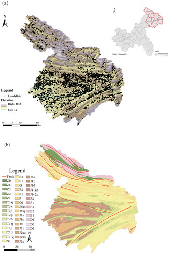
The study area, adjacent to Shaanxi, Sichuan, and Hubei provinces, is located between 30°29'23″ N–32°12'16″ N and 108°15'23″ E–110°11'37″ E and comprises five counties: Fengjie, Chengkou, Wushan, Wuxi, and Yunyang (Figure 1a). The study area is located to the east of the Sichuan Basin, with a complex landform. The landform is mainly mountainous and hilly, with an average altitude of 1,093 m. Structurally, certain areas of Wuxi and Chengkou are located in the Qinling geosyncline fold belt, while the remaining area is located in the northwest region of the Yangtze platform. Figure 1(b) shows the distribution of faults and lithology. From bottom to top, the Sinian, Cambrian, Ordovician, Silurian, Permian, Triassic, Jurassic, and Quaternary strata in the study area were successively developed. Most Devonian, Carboniferous, and Tertiary strata were missing. The study area has a subtropical monsoon climate, with sufficient rainfall and a warm climate. The annual average temperature is approximately 16 °C and the annual average rainfall exceeds 1,000 mm. The rainfall is mainly concentrated in summer, accounting for more than 30% of the total annual rainfall.

Figure 1. Landslide distribution and the geological map of the study area. (a) Location and historical landslide events distribution and (b) geological map.

2.1.1. Data and data sources

Data of the 3,758 historical landslides caused by rainfall events during this study period were obtained from the Chongqing geological monitoring station from 2001 to 2016 and were handled as point data; land use, administrative division, satellite images, digital elevation model (DEM) data, and other data were obtained from the Geographical Information Monitoring Cloud Platform. Land use data for 2015 were obtained while satellite images were obtained during the summer of 2016, when landslides were highly active. Geological data were obtained from the National Geological Archives Data Center. River network and road data were obtained from relevant monitoring departments in Chongqing in 2016. Annual average rainfall data were obtained for 2000–2014 from 72 meteorological stations by Chongqing Meteorological Administration. Point of interest (POI) data were captured using web crawler technology in 2016. The specific sources and data details are listed in Table 2.

Table 2. Data sources.

Data name	Data source	Type	Scale
Historical landslides	Chongqing geological monitoring station	Datasheet
DEM	Aster satellite	Grid	30 m
Geological data	National Geological Data Center	Grid	1:200,000
Land use	Geographical Information Monitoring Cloud Platform	Vector	1:100,000
Administrative division	Geographical Information Monitoring Cloud Platform	Vector	1:100,000
River networks	Chongqing Water Resources Bureau	Vector	1:100,000
Annual rainfall	Chongqing Meteorological Administration	Grid	30 m
Roads	Chongqing Transportation Commission	Vector	1:100,000
Satellite images	Geospatial Data Cloud	Grid	30 m
POI	Web Crawler	Datasheet

2.1.2. Landslide conditioning factors

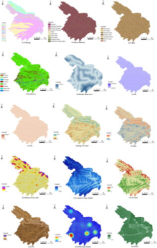
According to previous studies and the characteristics of the study area, 15 landslide factors were identified, including the lithology (X1), micro landforms (X2), combination reclassification of stratum dip direction and slope aspect (CRDS) (X3), landcover (X4), distance from the rivers (X5), stream power index (SPI) (X6), sediment transport index (STI) (X7), degree of relief (X8), aspect (X9), distance from the roads (X10), annual average rainfall (X11), elevation (X12), terrain roughness index (TRI) (X13), POI kernel density (X14), and normalized difference vegetation index (NDVI) (X15).

Lithology can reflect the softness of the soil and its water content in the landslide. Referring to previous studies (Yu et al. 2021; Liao et al., 2022), based on the digital map from the National Geological Data Center (http://dc.ngac.org.cn/Home), we vectorized digital map using ArcGIS and assigned values to different lithologies to obtain the lithology data of the study area. Micro landforms are a small-scale geomorphic forms, which affect the stability of side slope (Nhu et al. 2020). CRDS is the type of relationship between aspect and rock tendency, which is an important factor affecting landslides (Sun et al. 2020b). Land cover represents vegetation and land use patterns, both of which may affect susceptibility (Yu et al. 2021). The distance from the river quantifies the intensity of the river effects for the landslide; the closer to the river the landslide is, the higher the water content of the slope, the more serious the softening, while the slope stability decreases, it was calculated by the euclidean distance tool in ArcGIS. SPI can quantitatively describe the erosion capacity of surface water. The results include the path formed by the flow convergence and the possible erosion gully points. The larger the SPI value, the stronger the erosion ability of the surface water flow (Sestraș et al. 2019; Yu et al. 2019). STI can be used to characterize the transport and deposition of surface materials with water flow (Pourghasemi et al. 2012; Jiang et al. 2018), it was calculated by the hydrological analysis in ArcGIS. Degree of relief can be used to macroscopically describe the terrain. Aspect reflects the number of hours of sunlight available to the slope and impacts the vegetation growth condition. Distance from the road reflects the stability of the foot of the slope by the construction of the road. The annual average rainfall affects soil erosion and vegetation growth. Elevation is closely related to human activities, most of which are associated with lower elevations, making the geological structure of the area less affected (Yang et al. 2022). TRI can describe the surface morphology macroscopically. POI kernel density can reflect the influence of human activities, it was calculated by the nuclear density analysis tool in ArcGIS. NDVI can describe vegetation cover on the landslide surface and the root of vegetation can deepen soil stability (Jacquemart and Tiampo 2021) and was calculated based on Landsat images.

To unify the pixel size of all data, all data were resampled using ArcGIS software with CUBIC method. The 15 conditioning factors were input to the model at a resolution of 100 m, the number of pixels was 1,799,038, number of rows was 1,925, and number of columns was 1,825. They were reclassified using natural breakpoints, which can effectively avoid the uncertainties caused by data classification processing in the LSM (Huang et al. 2022). A landslide factor database was established by combining the reclassification results and historical landslides (Figure 2).

Figure 2. Thematic layers of landslide conditioning factors.

2.2. Methodology

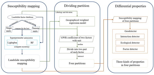
Figure 3 illustrates the process of this study, which includes the following three steps: First, data on landslides, elevation, remote sensing images, and data required for constructing a geospatial database were collected. LSM was applied using RF and LGBM on TUs and SUs. Moreover, the accuracy, mean square error (MSE), area under curve (AUC), and running time were evaluated. Second, the GWR was used to explore the coefficient of elevation and lithology on the landslide susceptibility, dividing the study area into four sub-regions. Finally, in each sub-region, the driving factors of landslide spatial distribution were determined using GeoDetector, which to insight the spatial differential characteristics of landslides.

Figure 3. The flowchart of the study methods.

2.3. Division method of evaluation units

2.3.1. Slope units

The SUs use crest and valley lines as division basis to divide the entire region into different sub-regions, which have been previously used (Camilo et al. 2017; Schlögel et al. 2018; Zhou et al. 2022). In this study, r.slopeunits software was used to divide the SUs, which can better extract the SUs in the study area (Alvioli et al. 2016). Two parameters, a and c, have a great impact for the result of SUs. We selected parameters a (50,000 m², 250,000 m², 500,000 m², 750,000 m², and 1,000,000 m²) and c (0.1, 0.2, 0.3, 0.4, 0.5, and 0.6) to run the r.slopeunits software for SUs. After continuous combination of a and c as the parameters of r.slopeunits software, the result was optimal when a was 50,000 m² and c was 0.4.

2.3.2. Terrain units

The methods to obtain the TUs have been previously proposed by Yan et al. (2017). Using the basic morphological principle of watershed segmentation by elevation and its derived variables and curvature, TUs were obtained by superimposed and inverse curvature of watershed boundaries according to the ArcGIS. The method not only uses ridgelines and valley lines for delineating TUs but also terraces valley boundaries to divide horizontal and sloping surfaces. The units are relatively uniform in size, with a shape generally between circular and triangular.

2.4. Susceptibility model

2.4.1. Light Gradient Boosting Machine (LGBM)

LGBM is a gradient lifting framework based on the decision tree first proposed by Microsoft and has been further optimized based on XGBoost. It exhibits high accuracy, high running speed, and small memory occupation (Chen et al. 2019). The basic learner of LGBM is a decision tree expressed as follows: (1) $$H_T\left(x\right)=\sum _{t=1}^T{H}_t\left(x\right),\mathrm{ }{H}_t\in \vartheta ,$$(1) where H_T is the ith learner and $\vartheta$ is a collection of learners.

LGBM was constructed in the form of a weighted linear combination of a series of decision trees, combining the weights of all leaf nodes to construct the tree. It traverses the samples based on the decision tree algorithm of the histogram, discretizes the floating-point eigenvalues into K integer spaces, and when traversing data, traverses the K spaces according to the discretized value as an index to identify the optimal sub-region point. First, it abandons the level-wise decision tree growth strategy used by most Geodatabase toolset tools and uses the leaf-wise algorithm with depth constraints. The leaf-wise algorithm identifies the leaf with the largest splitting gain from all the current leaves each time, and then splits. This cycle increases the depth and prevents overfitting. It can reduce more errors and obtain better accuracy. Gradient-based One-Side Sampling (GOSS) and Exclusive Feature Bundling (EFB) are used to reduce the number of samples and features required in the training process. GOSS can reduce a large number of data instances with only small gradients and obtain accurate information. Furthermore, EFB can bind many mutually exclusive features into one feature for dimension reduction. LGBM accelerates computation with optimized feature parallelism and data parallelism. When the data volume is very large, the voting parallelism strategy can also be used (Chen et al. 2019; Sahin 2022).

2.4.2. Random Forest

RF is a classifier that uses multiple decision trees to train samples. It was first proposed by Breiman (1996) and Cutler et al. (2012). The decision tree based on training samples and feature sets is the basic classifier of the RF algorithm. The decision tree combines the original data to build the decision tree models of different sub-datasets. According to the voting results, a group of construction models with the highest accuracy is selected to determine and predict the research results of the entire area. The essence of the stochastic forest model is to construct multiple decision trees to vote on the samples and select the mode from the voting results. In addition, RF can learn data quickly, can handle high-dimensional data, and can be easily parallelized (Genuer et al. 2017; Taalab et al. 2018; Sun et al. 2022). It is widely used in the study of LSM (Cao et al. 2019; Oliveira et al. 2019; Yang et al. 2022).

2.5. Validation method

To objectively compare each model, this study used the MSE, accuracy, time, and AUC to evaluate the performance of a model. MSE can reflect a degree of variation between predicted and true values. Accuracy is calculated based on the confusion matrix. Accuracy implies the proportion of positive and negative cells that are correctly classified. After the model was constructed, AUC, accuracy and MSE were calculated. Time could measure how fast the model runs, while AUC was the area of the ROC curve. The horizontal coordinate of the ROC curve is the False Positive Rate and the vertical coordinate is the True Positive Rate. The greater the AUC, better is the model. These factors have been used in previous LSM research to evaluate the accuracy and uncertainty of the LSM model (Huang et al. 2021b, 2022). The equation of MSE and accuracy is as follows: (1) $$\mathrm{Accuracy}=\frac{TP+TN}{TP+NP+TN+FN}$$(1) where FP is false positive and FN is false negative, both of which are the number of misclassified samples; moreover, TP is true positive and TN is true negative, both of which are the number of correctly classified samples. (2) $$\mathrm{MSE}=\sum _{i=1}^n{(Y_i-{\widehat{Y}}_i)}^2$$(2) where n is the number of samples, $Y_i$ is a real value, and ${\widehat{Y}}_i$ is a predicted value.

2.6. Dividing sub-regions—geographical weighted regression

GWR is a spatial analysis technique used in geography research, which explores the spatial variability of a study object at a given scale and the associated drivers by establishing a local regression equation at each point on a spatial scale. It has the advantage of greater accuracy as it considers the local effects of the spatial object. GWR can also be used to explore the relationship between dependent and independent variables (Yu and Gao 2020; He et al. 2021). The regression equation is as follows: (2) $$y_i={\beta }_0\left(u_i+v_i\right)+\sum _{k=1}^p{\beta }_k\left(u_i,v_i\right)x_{ik}+{\epsilon }_i\mathrm{ }i=1,2,\dots ,n$$(2) $\left(u_i+v_i\right)$ is the i coordinate of the sampling point, and ${\beta }_k\left(u_i,v_i\right)$ is the kth regression parameter on sampling point i, which is a function of geographical location obtained using the method of weight function in the estimation process.

To ensure the convenience of operation, the X and Y coordinates of each SU or TU on ArcGIS were collected, thus, obtaining statistical data on its susceptibility, elevation value, and lithology and recording the output in a table. In GWR4 software, the susceptibility was considered as a dependent variable, elevation, and lithology, which are the terrain factors, were considered independent variables, and the X and Y coordinates were considered spatial characteristic inputs. Subsequently, variable Gaussian Kernel function was set as the kernel function of weighted regression. The lithology and elevation coefficients were obtained through software calculation and used to determine whether the same region could be used. In ArcGIS, two types of coefficients were reclassified. The reclassified threshold values of the lithology and elevation coefficients were −1.055 and −16.134, respectively. Those less than or equal to the threshold value, and those exceeding the threshold value were classified as two different types. The reclassification results of the two categories were combined to obtain four sub-regions, and the final region results were obtained via sorting and counting.

2.7. Differential characteristics—GeoDetector

GeoDetector is a mathematical and statistical method proposed by WangJinfeng in 2010 to reveal the spatial differential characteristics of geographical items and explain their driving forces (Wang et al. 2007; Isojunno et al. 2017). Since the model can explain the internal driving mechanism of complex phenomena and the results can discuss the causes of phenomena from multiple perspectives, GeoDetector has been widely used in the geographical sciences, such as for ecological environmental assessment and economic population distribution (Sun et al., 2022). The concept of GeoDetector is based on the assumption that if a factor plays an important role in a phenomenon, the spatial distribution of the factor and phenomenon follows the first law of geography. GeoDetector includes four detectors: a risk detector, factor detector, ecological detector, and interaction detector, of which we used three, namely the ecological, factor, and interaction detectors. Considering the 15 landslide factors as the independent variables and the values of LSM as the dependent variables, the differential characteristics of landslides in different regions under different detectors were explored. Compared to the factor importance of machine learning algorithms, geographic probes can better consider the correlation and causality of geographical things. It can explore the degree of contribution of each factor to the model more accurately.

The factor detector was mainly used to explore the spatial differentiation and explanation of a single factor on a landslide, which was measured using the q value. This indicated the importance of each factor. The value of each factor ranged from 0 to 1 and was calculated as follows: (3) $$q=1-\frac{\sum _{h=1}^L{N}_h{\sigma }_h^2}{N{\sigma }^2},$$(3) where q is the explanatory variable of the conditioning factor on the landslide; h = 1, …, L is the stratification of the variables, i.e. the classification or sub-regions; $N_h$ and N are the number of units in layer h and the entire area, respectively; and $\sigma h^2$ and ${\sigma }^2$ are the variances of the dependent variable values of layer h and the entire region, respectively.

The interaction detector was mainly used to analyze whether the interaction of the two factors is enhanced or weakened compared with their independent effects. Single factors $z_1$ and $z_2$ were calculated to obtain $q\left(z_1\right)$ and $q\left(z_2\right),$ based on which $q\left(z_1\cap z_2\right)$ was calculated.

The ecological detector was measured by the F statistics to determine whether there is a significant difference between the impacts of the two factors on the location of the landslide. The calculation formula was as follows: (4) $$F=\frac{N_{z1}\times (N_{z2}-1)\times \sum _{h=1}^{L_1}{N}_h{\sigma }_h^2}{N_{z2}\times (N_{z1}-1)\times \sum _{h=1}^{L_2}{N}_h{\sigma }_h^2},$$(4) where the F statistic indicates whether there is a difference between the influence of the two factors, z1 and z2, on the landslide location; $N_{z1}$ and $N_{z2}$ represent the sample sizes of the two factors, respectively; and $L_1$ and $L_2$ represent the grading numbers of the two factors, respectively.

3. Results

3.1. Evaluation units

Dividing the study area into evaluation units to form a single evaluation unit can better match the terrain. Upon superimposing the SUs, TUs, and DEM, the sub-regions and distribution of the landslide were observed to be consistent with the topography. At the same time, the trend of the boundary line of the TUs was similar to that of the SUs, but the TUs were a more refined delineation of the SUs. The comparison between the SUs and TUs is illustrated in Figure 4(a) and 4(b).

Figure 4. The comparison between the SUs and Tus. (a) SUs and (b) Tus.

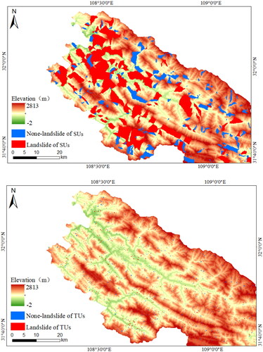
When a is 50,000 m² and c is 0.4, the DEM converges to the optimal sub-regions. In this case, the SUs achieve maximum internal homogeneity and external heterogeneity. The study area was divided into 19,712 SUs with a maximum unit area of 2,961 × 10⁴ m² and a minimum unit area of 5 × 10⁴ m²; the average unit area was 91 × 10⁴ m². The 3,758 historical landslides were located in 1,850 SUs selected as positive samples; 1,850 of the residual SUs were randomly selected as negative samples at a ratio of 1:1.

Using the TUs division method, the study area was divided into 524,742 small units. The maximum unit area was 26 × 10⁴ m², the minimum unit area was 1 × 10⁴ m², and the average unit area was 3 × 10⁴ m². There were 3,622 TUs with historical landslide positions; hence, these were selected as positive samples for training, and negative samples were selected at a ratio of 1:1.

3.2. Model evaluation and landslide susceptibility mapping

Units containing historical landslides were considered as positive samples and assigned a value of 1. According to the 1:1 ratio, units that do not contain historical landslides were randomly selected as negative samples and a value of 0 was assigned to them. Moreover, statistically relevant conditioning factors were analyzed using ArcGIS, and subsequently, input into each model. To determine the accuracy and capability of different evaluation units and models, accuracy, MSE, AUC values, and running time were used as the evaluation metrics. The evaluation results for each model are shown in Table 3 and the confusion matrix for each model are shown in Table 4. From the perspective of the evaluation unit, the accuracy of TUs under the same model exceeded that of SUs, while the MSE value of TUs was relatively small. Therefore, the use of TUs as evaluation units to establish the LSM model was more scientific. From the perspective of the model, the average accuracy of the LGBM model (0.7525) exceeded that of the RF model (0.743), and the LGBM model overcame the overfitting problem better. In conclusion, the LGBM model was more reliable and stable for LSM. Therefore, LGBM-TUs were selected for LSM, and specificity was studied on this basis.

Table 3. Evaluation metrics for different susceptibility models.

Type	RF-SUs	RF-TUs	LGBM-SUs	LGBM-TUs
Accuracy	0.738	0.748	0.743	0.762
MSE	0.262	0.252	0.257	0.238
AUC (training)	1.000	1.000	0.862	0.856
AUC (test)	0.814	0.815	0.803	0.829
Time	0.45 s	0.44 s	0.02 s	0.02 s

Table 4. The confusion matrix for different susceptibility models.

Model			Actual value
			Non-landslide (0)	Landslide (1)
RF-SUs	Predicted value	Non-landslide (0)	383	171
		Landslide (1)	120	436
RF-TUs	Predicted value	Non-landslide (0)	794	296
		Landslide (1)	251	832
LGBM-SUs	Predicted value	Non-landslide (0)	386	168
		Landslide (1)	117	439
LGBM-TUs	Predicted value	Non-landslide (0)	800	289
		Landslide (1)	228	856

LGBM-TUs were used to predict landslide susceptibility in the study area, and referring to previous studies (Baeza et al. 2016; Wang et al. 2021), the results were reclassified based on expert experience (Figure 5). By combining the objective results of machine learning computation with the expert’s prior knowledge, the LSM was divided into five susceptibility classes. According to statistical data of the area (Table 5), the number of landslides, and the density of landslides in different classes, the higher the susceptibility level, the smaller the area of the class; moreover, the strength of susceptibility and the area of the class were inversely proportional. The area of the very high susceptibility class (2,184.3 km²) was only half that of the very low susceptibility class (4,566.3 km²), but its landslide density (0.60) was 300 times that of the very low susceptibility class (0.02). The statistics showed that the LSM results were reliable.

Figure 5. Landslide susceptibility map based on LGBM-TUs.

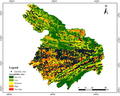
Table 5. Statistical results of landslide susceptibility classification.

Landslide probability	Susceptibility class	Area (km^2)	Number of landslides	Density (Pcs/km^2)
≤0.32	Very low	4,566.3	105	0.02
0.32–0.45	Low	4,006.2	220	0.05
0.45–0.62	Moderate	3,769.7	699	0.19
0.62–0.68	High	3,488.3	1,420	0.41
≥0.68	Very high	2,184.3	1,314	0.60

3.3. Dividing sub-regions

Using the GWR, the study was divided into four sub-regions, as shown in Figure 6. The characteristics of each sub-region of the statistics are shown in Table 6. The lithology of Sub-region 1 mainly comprises hard layered clastic rock and carbonate rocks, with a minimum area of 4,173.0 km². It is mainly located in Fengjie and Wushan counties, with an average elevation of 826.8 m. The area of Sub-region 2 is 4,967.8 km², with a minimum average elevation of 702.3 m, occupying the vast majority of the Yunyang area, mainly distributed with harder layered clastic rock and carbonate rock. Sub-region 3 is mainly located in Wuxi and Fengjie counties, with an area of 4,385.2 km² and an average elevation of 1,319.8 m. The main lithology comprises hard, layered carbonate rock. The entire Chengkou county and part of the Wuxi area belong to Sub-region 4. The lithology mostly comprises carbonate rock and a clastic complex, with an area of 4,488.8 km² and a maximum average elevation of 1,550 m. Among the four sub-regions, Sub-region 2 had the largest number of historical landslides, with 1,741 landslides; followed by Sub-regions 1, 4, and 3, with 1,491, 269, and 257 landslides, respectively. Sub-region 1 had the highest landslide density, 0.357 Pcs/km², while Sub-region 3 had the lowest (0.059 Pcs/km²).

Figure 6. Differences in the sub-regions of the study.

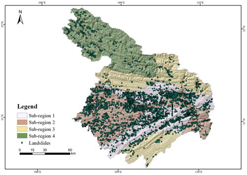
Table 6. Sub-region characteristics.

Type	Area (km^2)	Landslides	Landslide density (Pcs/km^2)	Average elevation (m)	Lithology
Sub-region 1	4,173	1,491	0.357	826.8	Hard layered clastic rock and carbonate rock
Sub-region 2	4,967.8	1,741	0.350	702.3	Harder layered clastic and carbonate rock
Sub-region 3	4,385.2	257	0.059	1,319.8	Hard layered carbonate rock
Sub-region 4	4,488.8	269	0.060	1,550	Carbonate rock and clastic complex

3.4. Differential characteristics

The interaction detector was mainly used to analyze whether the interaction of the two factors was enhanced or weakened compared with their independent effects. The results are shown in Figure 7. The results show that any combination of two factors can enhance the impact of the landslide. With respect to landslide occurrence, each factor does not act independently, but interacts with each other. Generally, the interaction intensity of lithology, annual average rainfall, and elevation with other factors is higher than those of the other factors.

Specifically, compared with other interactions, the values of the interaction between STI and SPI (0.029 and 0.024) were the lowest in Sub-regions 1 and 2, and the values of the TRI and slope were the lowest (0.022 and 0.020) in Sub-regions 3 and 4, indicating that the common influence of these two factors on landslides was less than that of the combination of other factors. Comparison of the influence degree of different factors and other factor combinations showed differences between the sub-regions. The slope factor in Sub-region 1 and NDVI in Sub-region 2 were the most significant, while the degrees of relief in Sub-regions 3 and 4 were consistent with the results of the single factor analysis. The above conditioning factors are expected to produce a variety of changes under complex conditions, which would have a significant impact on the landslides.

The ecological detector was determined by comparing whether there was a significant difference between two factors in the spatial distribution of landslides. The results are shown in Figure 8. Except for Sub-region 4, the lithology and elevation influenced the location distribution of landslides, indicating that these two factors play an important role in the distribution of landslides.

Specifically, in Sub-region 1, lithology, average annual rainfall, and elevation had a significant impact on the location of the landslides, while the distance from the river and TRI tended to be insignificant. In Sub-region 2, the lithology and elevation have a significant impact, and the interaction of NDVI with other factors affects landslide location. In Sub-region 3, lithology, elevation, average annual rainfall, and distance from the road affected the landslide distribution independently, while STI and NDVI had no significant effects. In Sub-region 4, the distance from the river, the distance from the road, and the elevation had a significant impact on landslides, while the SPI, STI, and POI kernel density had no significant impacts.

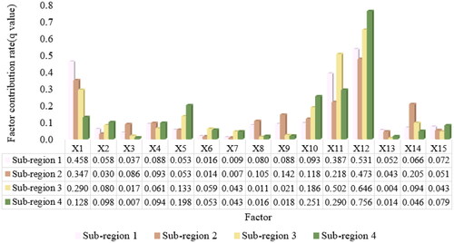
The factor detector can determine the impact of each factor on landslides. The results are shown in Figure 9. The results show that landslides are affected by landform, geological conditions, environmental conditions, and human activities. There were significant differences among the impacts of different impact factors on the occurrence of landslides, but the differences in the dominant factors in different sub-regions were small. Generally, the contribution rate of all factors to the occurrence of landslides ranges from 0.004 to 0.756. The influence of elevation, lithology, and annual average rainfall on the occurrence of landslides exceeds that of other single factors, while the contribution of three factors, SPI, STI, and degree of relief was relatively low. Lithology, elevation, and annual average rainfall are the dominant factors, which are consistent with the above interaction studies. The three factors interact and correlate with other factors, strengthening the impact of the occurrence of landslides.

4. Discussion

TUs were used as evaluation units, while the LGBM model was used to evaluate the LSM in the study area. We obtained the landslide susceptibility from an overall perspective, and the factor differentiation of the results was explored from a regional perspective, thereby providing a different research perspective for landslide susceptibility.

4.1. Rationality of the evaluation units and susceptibility model

The evaluation unit is the smallest LSM unit. Different evaluation units will affect the practical application of LSM. Selecting the appropriate evaluation unit will not only improve the accuracy of the model but also provide a strong guarantee for disaster prevention and control. In previous studies, GUs are often used as the evaluation units for LSM, but only consider size changes and cannot adequately describe changes in mountain morphology. In contrast, SUs and TUs consider elevation as the main data source for division. This evaluation unit is more suitable for the mountainous and hilly areas where the study area is located and can closely link the LSM with the landform. But there is a lack of comparison of SUs and TUs. To evaluate the advantages and disadvantages of the two evaluation units, we measured and compared the area, susceptibility, and accuracy. Table 3 and Figure 4 show that using TUs had more advantages.

The shape divided by the terrain was relatively more uniform, the difference between the maximum and minimum area was 26 times, while the difference between the SUs was 592 times. The average area of the TUs was 3 × 10⁴ m², which was closer to the historical landslide area. Simultaneously, under the same model, the accuracy of TUs slightly exceeded that of SUs, and the accuracies of the RF and LGBM models were 1.4% and 2.6% higher, respectively. In addition, this study divides the data for each evaluation unit into two parts: training and test sets. To comprehensively evaluate the performance of both models, the widely used AUC, accuracy, MSE and time were selected. The results show that the model built on TUs works more superiorly.

With the development of artificial intelligence technology, machine learning algorithms gradually tend to diversify. Selecting the suitable model is essential for LSM. The ensemble algorithm was obtained by combining multiple single learning models, integrating the advantages of a single learning model to obtain higher prediction accuracy (Ao et al. 2019). In our study, two ensemble learning algorithms that have been highly recognized were selected for comparison. The RF adopted Bagging to fuse multiple decision trees. As the optimization model of XGBoost, LGBM can shorten the training time and improve the prediction accuracy through GOSS, EFB, and other methods (Chen et al. 2019; Latha and Jeeva 2019). The AUC value, running time, accuracy, and MSE were analyzed. In Table 3, the LGBM model was superior to the RF model regardless of the statistical index. Therefore, the LGBM model was more reliable for LSM. In addition, the overall model was compared with each model based on each sub-region and by analyzing its accuracy, MSE, and AUC values; the results are listed in Table 7. The accuracy levels of Sub-regions 3 and 4 (0.780) exceeded the overall accuracy (0.762), but the accuracy levels of Sub-regions 1 and 2 were lower than the overall accuracy. Moreover, MSE and the two AUC values showed that the model accuracy of Sub-regions 1 and 2 were lower than that of the entire area, while Sub-regions 3 and 4 showed higher model accuracy than the entire area. The low accuracy levels of Sub-regions 1 and 2 may be related to the small number of landslides, while the number of landslides was less than 300. The information fed back by the data may be random and abnormal, resulting in the unsatisfactory learning effect of the model. To a certain extent, the LSM model based on sub-region can better characterize landslides and reflect their heterogeneity. Using a multi-scale study from an overall to a regional scale provides a new perspective for the study of landslides and a new method to optimize previous LSM.

Table 7. Statistical results at a regional and overall scale.

Type	MSE	Accuracy	AUC (training)	AUC (test)
Sub-region 1	0.312	0.688	0.831	0.767
Sub-region 2	0.349	0.651	0.793	0.682
Sub-region 3	0.220	0.780	0.910	0.861
Sub-region 4	0.220	0.780	0.888	0.846
Whole-region	0.238	0.762	0.856	0.829

4.2. Rationale for specificity studies at regional scales

Landslides are caused by the interaction of different natural environmental factors, and their occurrences are independent and unique, which show their spatial differential characteristics. Therefore, even for landslides with similar spatial locations, the mechanisms and inducing factors behind their occurrence may be quite different. Previous studies on landslides have been generally based on the whole-region, disregarding the spatial differential characteristics. Moreover, the whole-region is dominated by a single administrative region, while the administrative boundary is divided, which damages the integrity of some landforms. Therefore, combining multiple administrative regions, dividing the regional scale according to topographic conditions, and extending the research scale from overall to regional level is important for studying the spatial differential characteristics of landslides.

In this study, using the GWR to divide the study area into four sub-regions based on the spatial differential characteristics of the topographic conditions. And constructing models based on different sub-region. Table 7 demonstrates that the LSM model varies regionally and that the model accuracy of the LSM can be improved based on the sub-region. GeoDetector provides an insight into the linkages between landslides and conditioning factors in each sub-region, which can clarify the heterogeneity of landslides. Figures 7–9 show that different factors have different effects in different regions. Lithology, elevation, and annual average rainfall are the dominant factors, which largely determine the occurrence of landslides, since the rock determines the material basis of the landslide and controls the distribution of the landslide to a great extent. Rainfall washes and erodes the rock surface, and the leaked rainwater further erodes the interior of the slope and reduces its stability. In the study area, the forest area had relatively high elevation, with high vegetation coverage, marginal human activity-associated damage, and high rock mass stability. Moreover, under the influence of common action and interaction, the three factors enhance the influence of other factors on the landslide. Meanwhile, the aforementioned results are similar to those of previous studies (Sun et al. 2020a, 2021a, 2021b). Using GeoDetector to explore specificity provides a new perspective for the study of specificity and is important for exploring the mechanisms of landslide occurrence and for disaster prevention.

Figure 7. Results of the interaction detector based on the four sub-regions.

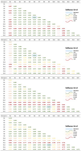
Figure 8. Results of ecological detector based on the four sub-regions.

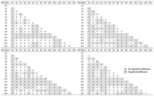
Figure 9. Results of factor detector based on the four sub-regions.

4.3. Study limitations and future outlook

To overcome the adverse impacts of administrative scale on the integrity of geomorphology, this study adopted the methods of sub-regions. It is important to predict landslide susceptibility based on different characteristics of landslides, which provides novel insights into LSM disaster prevention.

However, the number of selected districts and counties was limited, and additional districts and counties, such as parallel mountains and valleys or low mountains and hills, were not selected for sub-regions from the perspective of large-scale landforms. The selection of a large-scale study area allows for more optimized identification of the differences between landslides in different sub-regions and the elucidation of the controlling effect of landform on the stability and occurrence of landslides (Gorum et al. 2013). The preservation and impact of landforms on landslides remain to be assessed in future work. Additionally, hyperparameter optimization was not performed in this study. It can be obtained from Table 3. The modeling method used in this study exhibited high accuracy and could meet the requirements of the study.

GeoDetector was used to assess the specificity and insight the spatial correlation and specificity between the driving factors of landslides, although there are certain limitations. The classification number of the input data and discrete processing methods significantly affect the results of GeoDetector. GeoDetector can analyze the interactions between factors, but it cannot accurately determine the value. We will attempt to apply other methods when assessing the specificity of landslides in future studies.

Despite these limitations, the methods proposed in this study and the research on landslides in various sub-regions provide novel insights for LSM research. The methods adopted in this study can not only consider the spatial differential characteristics of landslides to improve the accuracy of the model but also explore the mechanism of landslide occurrence, which can effectively boost disaster prevention and control.

5. Conclusion

This study used a high-precision model to evaluate the LSM for the study area, and the landslide characteristics of each sub-region were studied comprehensively. In this study, TUs were regarded as the evaluation units, and the LGBM model was used to build the LSM model. Based on these results, in combination with the terrain conditions, the GWR was used to divide the sub-regions, and GeoDetector was used to study the spatial differential characteristics of each sub-region. The conclusions drawn are as follows:

1. The TUs surpass SUs in several aspects. The LSM based on LGBM-TUs was reliable with high accuracy and stability. It provides a novel reference method framework for LSM research.

2. Based on the GWR, the study area could be divided into different sub-regions based on the spatial differential characteristics of topography condition and prediction of the landslide susceptibility showed differences between sub-regions and whole-region, thus, suggesting new methods for LSM research.

3. GeoDetector can be used to study the characteristics of landslides in different sub-regions, which provides insights into the spatial differential characteristics of landslides.

4. In the future, we will apply other methods to accurately determine the role of each conditioning factor and elucidate the controlling effect of landform on the occurrence of landslides.

Disclosure statement

No potential competing interest was reported by the authors.

Data availability statement

The datasets used or analyzed during the current study are available from the corresponding author on reasonable request.

Additional information

Funding

This work was supported by Natural Science Foundation of Chongqing and China National Key R & D Program.

References

- Abbaszadeh Shahri A, Maghsoudi Moud F. 2021. Landslide susceptibility mapping using hybridized block modular intelligence model. Bull Eng Geol Environ. 80(1):267–284.
- Abbaszadeh Shahri A, Spross J, Johansson F, Larsson S. 2019. Landslide susceptibility hazard map in southwest Sweden using artificial neural network. CATENA. 183:104225.
- Alvioli M, Marchesini I, Reichenbach P, Rossi M, Ardizzone F, Fiorucci F, Guzzetti F. 2016. Automatic delineation of geomorphological slope units with r.slopeunits v1.0 and their optimization for landslide susceptibility modeling. Geosci Model Dev. 9(11):3975–3991.
- Ao Y, Li H, Zhu L, Ali S, Yang Z. 2019. The linear random forest algorithm and its advantages in machine learning assisted logging regression modeling. J Pet Sci Eng. 174:776–789.
- Baeza C, Lantada N, Amorim S. 2016. Statistical and spatial analysis of landslide susceptibility maps with different classification systems. Environ Earth Sci. 75(19):1318.
- Breiman L. 1996. Bagging predictors. Mach Learn. 24(2):123–140.
- Camilo DC, Lombardo L, Mai PM, Dou J, Huser R. 2017. Handling high predictor dimensionality in slope-unit-based landslide susceptibility models through LASSO-penalized Generalized Linear Model. Environ Model Softw. 97:145–156.
- Can R, Kocaman S, Gokceoglu C. 2021. A comprehensive assessment of XGBoost algorithm for landslide susceptibility mapping in the upper basin of Ataturk Dam, Turkey. Appl Sci. 11(11):4993.
- Cao J, Zhang Z, Wang C, Liu J, Zhang L. 2019. Susceptibility assessment of landslides triggered by earthquakes in the Western Sichuan Plateau. CATENA. 175:63–76.
- Chen C, Zhang Q, Ma Q, Yu B. 2019. LightGBM-PPI: predicting protein-protein interactions through LightGBM with multi-information fusion. Chemometr Intell Lab Syst. 191:54–64.
- Cutler A, Cutler DR, Stevens JR. 2012. Random Forests. In: Zhang C, Ma Y, editors. Ensemble machine learning: methods and applications. Boston, MA: Springer US. p. 157–175.
- Deng H, Wu X, Zhang W, Liu Y, Li W, Li X, Zhou P, Zhuo W. 2022. Slope-unit scale landslide susceptibility mapping based on the random forest model in deep valley areas. Remote Sens. 14(17):4245.
- Dou J, Yunus AP, Bui DT, Merghadi A, Sahana M, Zhu Z, Chen C-W, Khosravi K, Yang Y, Pham BT. 2019. Assessment of advanced random forest and decision tree algorithms for modeling rainfall-induced landslide susceptibility in the Izu-Oshima Volcanic Island, Japan. Sci Total Environ. 662:332–346.
- Froude MJ, Petley DN. 2018. Global fatal landslide occurrence from 2004 to 2016. Nat Hazards Earth Syst Sci. 18(8):2161–2181.
- Ge Y, Chen H, Zhao B, Tang H, Lin Z, Xie Z, Lv L, Zhong P. 2018. A comparison of five methods in landslide susceptibility assessment: a case study from the 330-kV transmission line in Gansu Region, China. Environ Earth Sci. 77(19):662.
- Genuer R, Poggi J-M, Tuleau-Malot C, Villa-Vialaneix N. 2017. Random Forests for Big Data. Big Data Res. 9:28–46.
- Gorum T, van Westen CJ, Korup O, van der Meijde M, Fan X, van der Meer FD. 2013. Complex rupture mechanism and topography control symmetry of mass-wasting pattern, 2010 Haiti earthquake. Geomorphology. 184:127–138.
- He X, Mai X, Shen G. 2021. Poverty and physical geographic factors: an empirical analysis of Sichuan Province using the GWR model. Sustainability. 13(1):100.
- Huang F, Cao Z, Guo J, Jiang S-H, Li S, Guo Z. 2020a. Comparisons of heuristic, general statistical and machine learning models for landslide susceptibility prediction and mapping. CATENA. 191:104580.
- Huang F, Cao Z, Jiang S-H, Zhou C, Huang J, Guo Z. 2020b. Landslide susceptibility prediction based on a semi-supervised multiple-layer perceptron model. Landslides. 17(12):2919–2930.
- Huang F, Pan L, Fan X, Jiang S-H, Huang J, Zhou C. 2022. The uncertainty of landslide susceptibility prediction modeling: suitability of linear conditioning factors. Bull Eng Geol Environ. 81(5):182.
- Huang F, Tao S, Chang Z, Huang J, Fan X, Jiang S-H, Li W. 2021a. Efficient and automatic extraction of slope units based on multi-scale segmentation method for landslide assessments. Landslides. 18(11):3715–3731.
- Huang F, Ye Z, Jiang S-H, Huang J, Chang Z, Chen J. 2021b. Uncertainty study of landslide susceptibility prediction considering the different attribute interval numbers of environmental factors and different data-based models. CATENA. 202:105250.
- Huang F, Zhang J, Zhou C, Wang Y, Huang J, Zhu L. 2020c. A deep learning algorithm using a fully connected sparse autoencoder neural network for landslide susceptibility prediction. Landslides. 17(1):217–229.
- Huang Y, Zhao L. 2018. Review on landslide susceptibility mapping using support vector machines. Catena. 165:520–529.
- Isojunno S, Sadykova D, DeRuiter S, Cure C, Visser F, Thomas L, Miller PJO, Harris CM. 2017. Individual, ecological, and anthropogenic influences on activity budgets of long-finned pilot whales. Ecosphere. 8(12):e02044.
- Jacquemart M, Tiampo K. 2021. Leveraging time series analysis of radar coherence and normalized difference vegetation index ratios to characterize pre-failure activity of the Mud Creek landslide, California. Nat Hazards Earth Syst Sci. 21(2):629–642.
- Jiang S-H, Huang J, Huang F, Yang J, Yao C, Zhou C-B. 2018. Modelling of spatial variability of soil undrained shear strength by conditional random fields for slope reliability analysis. Appl Math Modell. 63:374–389.
- Jones S, Kasthurba AK, Bhagyanathan A, Binoy BV. 2021. Landslide susceptibility investigation for Idukki district of Kerala using regression analysis and machine learning. Arab J Geosci. 14(10):838.
- Latha CBC, Jeeva SC. 2019. Improving the accuracy of prediction of heart disease risk based on ensemble classification techniques. Inf Med Unlocked. 16:100203.
- Liao M,Wen H,Yang L. 2022. Identifying the essential conditioning factors of landslide susceptibility models under different grid resolutions using hybrid machine learning: A case of Wushan and Wuxi counties, China. CATENA. 217:106428.
- Min D-H, Yoon H-K. 2021. Suggestion for a new deterministic model coupled with machine learning techniques for landslide susceptibility mapping. Sci Rep. 11(1):6594.
- Nhu V-H, Shirzadi A, Shahabi H, Singh SK, Al-Ansari N, Clague JJ, Jaafari A, Chen W, Miraki S, Dou J, et al. 2020. Shallow landslide susceptibility mapping: a comparison between logistic model tree, logistic regression, Naïve Bayes tree, artificial neural network, and support vector machine algorithms. IJERPH. 17(8):2749.
- de Oliveira GG, Ruiz LFC, Guasselli LA, Haetinger C. 2019. Random forest and artificial neural networks in landslide susceptibility modeling: a case study of the Fão River Basin, Southern Brazil. Nat Hazards. 99(2):1049–1073.
- Pham BT, Bui DT, Prakash I, Dholakia MB. 2017. Hybrid integration of Multilayer Perceptron Neural Networks and machine learning ensembles for landslide susceptibility assessment at Himalayan area (India) using GIS. Catena. 149:52–63.
- Pham BT, Vu VD, Costache R, Phong TV, Ngo TQ, Tran T-H, Nguyen HD, Amiri M, Tan MT, Trinh PT, et al. 2022. Landslide susceptibility mapping using state-of-the-art machine learning ensembles. Geocarto Int. 37(18):5175–5200.
- Pourghasemi HR, Mohammady M, Pradhan B. 2012. Landslide susceptibility mapping using index of entropy and conditional probability models in GIS: safarood Basin, Iran. CATENA. 97:71–84.
- Rong G, Alu S, Li K, Su Y, Zhang J, Zhang Y, Li T. 2020. Rainfall induced landslide susceptibility mapping based on Bayesian optimized Random Forest and gradient boosting decision tree models – a case study of Shuicheng County, China. Water. 12(11):3066.
- Saber M, Boulmaiz T, Guermoui M, Abdrabo KI, Kantoush SA, Sumi T, Boutaghane H, Nohara D, Mabrouk E. 2021. Examining LightGBM and CatBoost models for wadi flash flood susceptibility prediction. Geocarto Int. 37(25):7462–7487.
- Sahin EK. 2022. Comparative analysis of gradient boosting algorithms for landslide susceptibility mapping. Geocarto Int. 37(9):2441–2465.
- Schlögel R, Marchesini I, Alvioli M, Reichenbach P, Rossi M, Malet J-P. 2018. Optimizing landslide susceptibility zonation: effects of DEM spatial resolution and slope unit delineation on logistic regression models. Geomorphology. 301:10–20.
- Sestraș P, Ștefan B, Roșca S, Naș S, Bondrea MV, Gâlgău R, Vereș I, Sălăgean T, Spalević V, Cîmpeanu SM. 2019. Landslides susceptibility assessment based on GIS statistical bivariate analysis in the hills surrounding a metropolitan area. Sustainability. 11(5):1362.
- Sun D,Gu Q,Wen H,Xu J,Zhang Y,Shi S,Xue M,Zhou X. 2022. Assessment of landslide susceptibility along mountain highways based on different machine learning algorithms and mapping units by hybrid factors screening and sample optimization. Gondwana Res. 10.1016/j.gr.2022.07.013.
- Sun D, Gu Q, Wen H, Shi S, Mi C, Zhang F. 2022. A hybrid landslide warning model coupling susceptibility zoning and precipitation. Forests. 13(6):827.
- Sun D, Shi S, Wen H, Xu J, Zhou X, Wu J. 2021a. A hybrid optimization method of factor screening predicated on GeoDetector and Random Forest for Landslide Susceptibility Mapping. Geomorphology. 379:107623.
- Sun D, Wen H, Wang D, Xu J. 2020a. A random forest model of landslide susceptibility mapping based on hyperparameter optimization using Bayes algorithm. Geomorphology. 362:107201.
- Sun D, Xu J, Wen H, Wang D. 2021b. Assessment of landslide susceptibility mapping based on Bayesian hyperparameter optimization: a comparison between logistic regression and random forest. Eng Geol. 281:105972.
- Sun D, Xu J, Wen H, Wang Y. 2020b. An optimized Random forest model and its generalization ability in landslide susceptibility mapping: application in two areas of Three Gorges Reservoir. China. J Earth Sci. 31(6):1068–1086.
- Taalab K, Cheng T, Zhang Y. 2018. Mapping landslide susceptibility and types using Random Forest. Big Earth Data. 2(2):159–178.
- Wang Y, McElroy MB, Boersma KF, Eskes HJ, Veefkind JP. 2007. Traffic restrictions associated with the Sino-African summit: reductions of NOx detected from space: change in Beijing NOX by traffic control. Geophys Res Lett. 34(8):L08814.
- Wang Y, Sun D, Wen H, Zhang H, Zhang F. 2020. Comparison of Random Forest model and frequency ratio model for landslide susceptibility mapping (LSM) in Yunyang County (Chongqing, China). IJERPH. 17(12):4206.
- Wang Y, Wen H, Sun D, Li Y. 2021. Quantitative assessment of landslide risk based on susceptibility mapping using Random Forest and GeoDetector. Remote Sens. 13(13):2625.
- Yan G, Liang S, Zhao H. 2017. An approach to improving slope unit division using GIS technique. Scientia Geographica Sinica. 37(11):1764–1770.
- Yang C, Liu L-L, Huang F, Huang L, Wang X-M. 2022. Machine learning-based landslide susceptibility assessment with optimized ratio of landslide to non-landslide samples. Gondwana Res. https://doi.org/10.1016/j.gr.2022.05.012
- Yu L, Cao Y, Zhou C, Wang Y, Huo Z. 2019. Landslide susceptibility mapping combining information gain ratio and support vector machines: a case study from Wushan segment in the Three Gorges Reservoir Area, China. Appl Sci. 9(22):4756.
- Yu X, Gao H. 2020. A landslide susceptibility map based on spatial scale segmentation: a case study at Zigui-Badong in the Three Gorges Reservoir Area, China. PLoS One. 15(3):e0229818.
- Yu X, Zhang K, Song Y, Jiang W, Zhou J. 2021. Study on landslide susceptibility mapping based on rock–soil characteristic factors. Sci Rep. 11(1):15476.
- Zhang J, Ma X, Zhang J, Sun D, Zhou X, Mi C, Wen H. 2023. Insights into geospatial heterogeneity of landslide susceptibility based on the SHAP-XGBoost model. J Environ Manage. 332:117357.
- Zhao Y, Bai C, Xu C, Foong LK. 2021a. Efficient metaheuristic-retrofitted techniques for concrete slump simulation. Smart Struct Syst. 27(5):745–759.
- Zhao Y, Hu H, Bai L, Tang M, Chen H, Su D. 2021b. Fragility analyses of bridge structures using the logarithmic piecewise function-based probabilistic seismic demand model. Sustainability. 13(14):7814.
- Zhao Y, Hu H, Song C, Wang Z. 2022. Predicting compressive strength of manufactured-sand concrete using conventional and metaheuristic-tuned artificial neural network. Measurement. 194:110993.
- Zhao Y, Moayedi H, Bahiraei M, Foong LK. 2020. Employing TLBO and SCE for optimal prediction of the compressive strength of concrete. Smart Struct Syst. 26(6):753–763.
- Zhou X, Wen H, Li Z, Zhang H, Zhang W. 2022. An interpretable model for the susceptibility of rainfall-induced shallow landslides based on SHAP and XGBoost. Geocarto Int. 37(26): 13419–13450.