Optimizing soil erosion estimates of RUSLE model by analyzing land use/cover dynamics in upper Awash River Basin, Central Ethiopia

Abstract

The Revised Universal Soil Loss Equation (RUSLE) is the most widely used erosion model for decision making on conservation priority. However, interpreting estimates of the mean annual soil loss alone could not accurately depict the spatial variation of soil erosion severity due to its inherent mathematical errors. This study aims to optimize the model’s outputs through detailed analysis of land use/cover dynamics in Upper Awash River Basin, central Ethiopia (7815.1 km²). The analysis include annual rate of change, net gain or loss, and conversion pathways. Results of the estimated mean annual soil loss in the basin varies between 4.1 t/ha/y and 5.1 t/ha/y during three consecutive decades (1990-2000, 2000-2010, and 2010-2020). The cultivated land cover exhibits slight erosion severity (< 5 t/ha/y), while contributing up to 59% the total annual soil loss (3198.8 Mt/ha). Although the net loss of cultivated land cover outweighing the gain during these decades, it progressively encroaches forests (142.2 km²), shrubs (780.8 km²), and grasslands (274.5 km²). Such net loss of protective land covers will inevitably increase the soil erosion risk. Findings from the study would be useful, enabling conservation practitioners to understand the overall severity of soil erosion and make informed decisions.

Keywords:

• The RUSLE model
• optimize
• mean annual soil loss
• erosion severity
• land use/cover
• Upper Awash River Basin

1. Introduction

Soil erosion by water remains the major cause of land degradation, making it the most serious environmental challenge worldwide. For example, a global assessment report has estimated the annual soil loss to be around 36 billion tons (Borrelli et al. 2017). According to the report, there was a 2.5% increase in soil erosion due to the conversion of forest to cropland between 2000 and 2012, indicating land use/cover (LULC) changes highly influence the rate of erosion. Additionally, the report predicts that Sub-Saharan Africa and South East Asia are expected to suffer the greatest losses.

Similarly, soil erosion is posing environmental and economic risks in Ethiopia, the second most populous nation in Africa. It is more severe in the highlands, where it accommodates about 90% of the human population and two-thirds of the cattle population (Yesuf et al. 2005). Earlier reports, for example, revealed a gross annual soil loss of 42 tons per hectare per year (t/ha/y) from the cultivated land alone, and varies between 0 and 300 t/ha/y on steep slopes (Hurni 1988). The mean annual soil loss was estimated to be 12 t/ha/y with a total of 1,493 million t/ha (Hurni 1988; Yesuf et al. 2005). Land degradation due to LULC change annually costs over $4.3 billion (Gebreselassie et al. 2015). It is a huge loss as agriculture accounts for about one-third of the country’s GDP and employs more than two-thirds of the population (World Bank 2007). Similarly, a recent review work on gross annual soil loss estimated to be 38 t/ha/y from crop land alone, and varies between 0 and 220 t/ha/y (Tamene et al. 2022). Moreover, climate change intensifies the prevailing challenge of soil erosion, affecting agricultural practices (Verstraeten et al. 2006; Kidane et al. 2019; Teshome and Zhang 2019).

This study was conducted in the Upper Awash River basin where soil erosion by water seriously threatening various environmental, economic, and social sectors. Several studies have been conducted in the basin such as hydrological process (Girma et al. 2015; Bekele et al. 2017; Birhanu et al. 2021; Tadesse and Dai 2019), analysis of dry and wet spells (Adane et al. 2020), impacts of climate change and population growth on river nutrient loads (Bussi et al. 2021), extent and spatiotemporal detection of LULC change (Shawul and Chakma 2019), analysis of regional trends of extreme precipitation indices and long-term climate variability (Shawul and Chakma 2020; Gebremichael et al. 2022), and modeling of land use dynamics (Tessema et al. 2020). For example, the recently documented spatiotemporal trend analysis of extreme precipitation events in the basin revealed increasing trends, which inevitably escalates the existing soil erosion hazards (Bekele et al. 2017; Dawit et al. 2019; Shawul and Chakma 2020; Mohamed et al. 2022; Abebe et al. 2022).

The basin accounts for about 36% of manufacturing values and 25% of the agricultural production in Ethiopia (Bekele et al. 2017; Vivid Economics 2016). It accommodates almost 6.2 million people, including the population of Addis Ababa, the country’s capital (Central Statistical Agency 2014). The Koka Hydroelectric Power Dam is also located in the downstream zone of the basin. It has played an important economic role since 1960, however, sedimentation due to upland erosion has reduced the dam’s actual storage capacity (1,850 million m³) by 35% (Honningsvag et al. 2001; Girma et al. 2015). This results in overland water flow. For example, the overflow of Koka, including Kesem and Tendaho has recently damaged more than 60,000 hectares of crops and farmlands (FloodList News 2020). Trends of extreme precipitation indices are also increasing in the basin (Shawul and Chakma 2020), which ultimately affects the regional economy and wildlife resources (Vivid Economics 2016; BirdLife International 2022).

In such cases, soil erosion models can play critical roles in proactively managing soil and water degradation in the basin. Several models have been developed, and can be classified as statistical, physical, process-based, and empirical models. Several models have been developed, and can be classified as statistical, physical, process-based, and empirical models. For example, Pandey et al. (2021) conducted a comprehensive review of 18 different models to summarize the recent methodological advances, their status and limitations. According to the authors, some of the most widely applied models in recent times include, the Revised Universal Soil Loss Equation (RUSLE), The Pan-European Soil Erosion Risk Assessment (PESERA), The Water Erosion Project (WEEP) Model, and the Soil and Water Assessment Tool (SWAT). Particularly, the RUSLE model is the top most used empirical model worldwide, estimating long-term sheet and rill erosion rates (e.g. Gelagay and Minale 2016; Molla and Sisheber 2017; Pham et al. 2018; Shi et al. 2020; Negese 2021; Getachew et al. 2021). Yet, only a few studies have attempted to associate soil erosion response to LULC change (Yan et al. 2018; Kidane et al. 2019; Getachew et al. 2021; Belay and Mengistu 2021). The model in general involves six input parameters (erosivity, erodibility, slope length, and steepness, cover management, and conservation practices). Its ability to integrate with remote sensing and GIS techniques makes it robust and adoptable, especially where data is scarce (Gelagay and Minale 2016; Benavidez et al. 2018).

However, the model is attributed by limitations. Some of its input parameters are subjective and inconsistent, resulting significant errors and uncertainties of the model output (Breiby 2006; Benavidez et al. 2018). For example, conservation practice (P) and cover management (C) factors mostly rely on expert judgment or previously published works (Benavidez et al. 2018). These parameters would rather change over time, making it challenging to obtain reliable values (Abdul Rahaman et al. 2015). The C factor also does not account for differences in plant species or root structure. Similarly, the erosivity (R) factor, which measures rain intensity and kinetic energy is not available in many regions of the world (Verstraeten et al. 2006). As a result, it is derived indirectly using average annual precipitation (Hurni 1985). In addition, depending on the physiographic characteristics of a watershed, the model may under or overestimate the rate of soil erosion. For example, as it does not account for sediment deposition, it predict higher mean erosion rate, particularly landscapes over a steep slope. On the other hand, it does not consider soil loss due to gully erosion and land mass, which underestimate the overall severity of soil erosion in a watershed (Benavidez et al. 2018). These limitations in general highlight the need for interpreting soil erosion vulnerability beyond magnitude of the mean annual soil loss, which otherwise misleads our decision on conservation priority.

Therefore, this study focuses on optimizing soil erosion estimates using the Revised Universal Soil Loss Equation (RUSLE) model with Land Use/Cover (LLULC) analysis. This would maintain the reliability of the model application for soil loss estimations, which ultimately provides robust information when decision-makers used to interpret soil loss risk.

2. Materials and methods

2.1. Study area

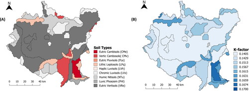
This study was conducted in the Upper Awash River basin, located in Central Ethiopia. It stretches between 8°10′ N, 8°50′ N Latitude and 38°00′ N, 39°00′ E Longitude, and covers a total land area of about 7815 km². Its elevation above sea level ranges from 1596 m to 3573 m (Figure 1). The major LULC types include cultivated land (81.7%), built-up areas (5.8%), bare lands (3.3%), grassland (1.8%), shrubs (6%), forest (1.3%), and water bodies (0.2%). The two main types of surficial lithology are silicic (19%) and volcanic ash, tuff, and mudflow (69.2%). A type of lithology strongly influences slope stability (Sarkar et al. 1995). The landforms are also mainly represented by smooth (28.2%) and irregular plains (38.3%). The major soil types also include Eutric Vertisols (56.7%), Humic Nitisols (14%), Chromic Luvisols (12%), and Lithic Leptosols (6.7%).

Figure 1. Location map of the study area.

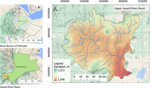
Based on the weather records (1987–2020) analysis, the weighted mean annual precipitation approximately equals 993.4 mm (788–1558 mm/year), and the mean annual temperature is 17.2 °C (13 - 21 °C). The climate is typically classified as humid subtropical to semi-arid, with significant seasonal variation in precipitation. It is influenced by the Inter-Tropical Convergence Zone (ITCZ), which creates the wet and dry seasons in the tropics (Halcrow 1989). The long rainy season (kiremt) runs from June to September, while the short rainy season (belg) runs from February to May.

2.2. Datasets and sources

Daily precipitation data (1987-2020) from 12 weather stations were obtained from the Ethiopian National Meteorological Agency (ENMA). Appendix 1 shows a summary information on the weather stations and mean annual rainfall of the study area. Of these, Asgori, Bantuliben, Boneya, Kimoye, and Lemen represent 80% of the basin land area.

A cloud-free (< 10%) multi-temporal Landsat imageries (LS5-TM and LS8-OLI; Path/Row 168 & 169/54) were accessed from achieves of the United States Geological Survey (USGS), available at https://earthexplorer.usgs.gov/. The Landsat images were used to create thematic maps of LULC for 1990, 2000, 2010, and 2020. Similarly, the Digital Elevation Model (DEM, 30 m) of the Shuttle Radar Topographic Mission (SRTM) was obtained from http://worldgrids.org/doku.php. The DEM was used to delineate the basin and derive topographic factors. Soil data needed to generate the soil erodibility (K-factor) obtained from FAO’s Harmonized World Soil Database (HWSD) v1.2 at 30 arcsec resolution (FAO Soil Portal 2019).

2.3. Data processing techniques

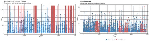
The rainfall datasets were preprocessed using spreadsheet Excel and R-programming languages platforms available at https://www.r-project.org. The operation involves cleaning raw data, imputation of missing values, and data arrangement for statistical analysis. The missing values of precipitation data were filled using univariate imputation techniques of “mice” package in the R programing language (Moritz and Bartz-Beielstein 2017). Classification and regression trees (CART) and predictive mean matching algorithms (pmm) were used for the imputation, which is relatively robust technique (Bailey et al. 2020). Sample outputs of this technique are presented in Appendix 2. In addition, geo-processing of the multi-temporal Landsat images was performed using image processing software: ArcGIS v10.6 and QGIS v3.22.1. They used to analyze, manipulate, query, re-project, and create the spatial thematic maps using remote sensing data. The Landsat imageries were projected to WGS_1984_UTM_Zone_37N, and image mosaic performed from which the study area was extracted.

2.4. Classification of LULC

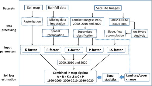
Following preprocessing of the Landsat imageries, optimal combinations of spectral bands were selected over the mosaic image. First, training samples for each class were gathered. These samples are homogeneous cluster of pixels, representing the predefined land use classes. Operational definitions of the LULC schemes are described in Appendix 4. The procedure involves field surveys, interpretation of Google Earth satellite imageries, and false color combinations of the Landsat images of 1990, 2000, 2010, and 2020. Based on the training sample dataset, the LULC classification was performed using Semi-Automatic supervised Classification Plugin (SCP) in QGIS Desktop 3.22.1 (Luca 2021), which embedded a Maximum Likelihood algorithm. Finally, some of incorrectly classified pixels were repeatedly refined to address better classification accuracy. Figure 2 shows the overall methodological framework of the study.

Figure 2. Methodology framework of the study.

Accuracy levels of the classified thematic maps were further evaluated by cross-tabulation between the class values and the reference pixels. For the classified map of 2020, a total of 281 ground control points (reference samples) were obtained from field survey and very high-resolution images using the Google Earth satellite database. A stratified sampling technique was used to represent each LULC class. To obtain an adequate number of reference samples (N) for each class, Olofsson et al. (2014) suggested Eq.1(Eq.1) $$N=(\sum _{c=i}^c(\text{Wi*Si})/\mathrm{So})2$$(Eq.1) : (Eq.1) $$N=(\sum _{c=i}^c(\text{Wi*Si})/\mathrm{So})2$$(Eq.1) where: W_i = mapped area proportion of class i; Si = standard deviation of stratum i; So = expected standard deviation of overall accuracy; c = total number of classes

The thematic maps were further used to create a LULC change-transition matrix using the same Plugin (SCP) in QGIS Desktop 3.22.1. The matrix is then used to compute the annual rate of LULC change. For ease of interpretation, Puyravaud (2003) proposed a more intuitive standardized formula (Equation 2(Eq. 2) $$\mathrm{r}=\frac{1}{t2-t1}\mathrm{\hspace{0.17em}*\hspace{0.17em}}ln\hspace{0.17em}\frac{A2}{A1}$$(Eq. 2) ). Batar et al. (2017) used the procedure, for example, to assess LULC change and forest fragmentation. (Eq. 2) $$\mathrm{r}=\frac{1}{t2-t1}\mathrm{\hspace{0.17em}*\hspace{0.17em}}ln\hspace{0.17em}\frac{A2}{A1}$$(Eq. 2)

Where A₂ and A₁ refer to the Area (sq. km) of land cover at t₂ and t₁, respectively.

However, for the 1990, 2000 and 2010 ground control points couldn’t be available. Thus, temporally invariant sample features were used to create an alternative reference dataset for validating these maps (Sabr et al. 2016). These authors resolved similar challenge without compromising the level of uncertainty.

2.5. Analysis of LULC dynamics

The LULC change is one of the most important physiographic watershed characteristics that determine soil erosion. Based on the multi-temporal classification analysis of the LULC schemes, post classification comparison of LULC change was also performed using SCP Plugin in QGIS (Luca 2021). The comparison purposefully sub-divided into three consecutive decades: 1990–2000, 2000–2010 and 2010–2020, with seven combination of “to-from” change detection. Sabr et al. (2016) used a similar procedure.

2.6. Description of RUSLE model and input parameter estimation

The spatial variation of soil erosion was estimated using the Revised Universal Soil Loss Equation (RUSLE) model (Renard et al. 1991), which is the most widely adopted empirical model. The recent advances in geospatial technologies provide robust platforms to this particular model. It can predict erosion potential on a cell-by-cell basis, and it is effective to identify the spatial pattern of soil loss within a large region (Breiby 2006). It is computed based on Equation 3(Eq.3) $$\mathrm{A}\mathrm{ }(\mathrm{t}/\mathrm{ha}/\mathrm{y})=\mathrm{R}\times \mathrm{K}\times \mathrm{LS}\times \mathrm{C}\times \mathrm{P}$$(Eq.3) : (Eq.3) $$\mathrm{A}\mathrm{ }(\mathrm{t}/\mathrm{ha}/\mathrm{y})=\mathrm{R}\times \mathrm{K}\times \mathrm{LS}\times \mathrm{C}\times \mathrm{P}$$(Eq.3)

Where:

A is the mean annual soil loss (t/ha/y),

R is the erosivity of rainfall (MJ.mm.ha.h.yr⁻¹),

K is the erodibility of soil (t.ha.h.ha⁻¹.MJ⁻¹.mm⁻¹),

LS is the topographic factor (dimensionless),

C is the cover management factor (dimensionless), and

P is the support practice factor (dimensionless)

2.6.1. Rainfall erosivity (R-factor)

The R-factor refers to the erosive force of a specific rainfall event that contributes to soil loss by raindrops (Wischmeier and Smith 1978). It is calculated as the sum of rainfall kinetic energy and maximum 30-minute rainfall intensity (EI₃₀). However, such precipitation data does not have a high temporal resolution, so values were computed using an empirical equation (Equation 4(Eq.4) $$\mathrm{R}\mathrm{ }=\mathrm{ }-8.12\mathrm{ }+\mathrm{ }\left(0.562\mathrm{*}\mathrm{P}\right)$$(Eq.4) ) developed for the Ethiopian highlands (Hurni 1985). (Eq.4) $$\mathrm{R}\mathrm{ }=\mathrm{ }-8.12\mathrm{ }+\mathrm{ }\left(0.562\mathrm{*}\mathrm{P}\right)$$(Eq.4) where: P is the mean annual rainfall in mm.

The annual rainfall dataset was used to calculate rainfall erosivity over three decades (1987–2000, 1998–2010, and 2008–2020). The periods are purposefully subdivided to correspond with the analysis of LULC change for each decade. However, spatial distribution of the rainfall erosivity was deliberately estimated with a lag period of at least two years from the corresponding lower cut-off year in the LULC interval (i.e. 1990, 2000 and 2010). This lag year is assumed to be sufficient to influence vegetation cover in semi-arid region (Wang et al. 2022), and hence considered in the analysis to buffer reliability of the rainfall data. A study also reveals a positive linear relationship between rainfall and Normalized Difference Vegetation Index (NDVI) in arid and semi-arid regions (Shisanya et al. 2011; Zerkani et al. 2022).

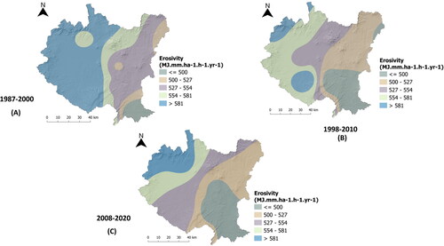
The values range from 428 to 1016 MJ.mm.ha⁻¹.h⁻¹.yr⁻¹. The computed mean annual rainfall data were interpolated using an inverse distance weighting (IDW) technique and then rasterized into a 30 m spatial resolution. Finally, the R-factor was computed for each pixel using a raster calculator in the QGIS v3.22.1 processing tool (Figure 3).

Figure 3. Spatial distribution of rainfall erosivity (R-factor) during (a) 1987–2000; (b) 1998–2010 and (c) 2008–2020.

2.6.2. Topography (LS-factor)

The topographic factor (slope length and steepness) was calculated using the Digital Elevation Model (DEM-30m) of the Shuttle Radar Topography Mission (SRTM). This factor reflects the connection between these factors and soil erosion. As slope length increases, soil loss per unit area also increases (Ganasri and Ramesh 2016). Moore and Wilson (1992) used to calculate the topographic factor (LS) using Equation 5(Eq.5) $$\mathrm{L} = {\left.\left( \frac{\mathbf{\lambda }}{22.13}\right.\right)}^m$$(Eq.5) and Equation 6(Eq.6) $$\mathrm{S}=\{\begin{array}{c}10.8\sin \hspace{0.17em}\mathrm{\theta }+0.03\\ 16.8\sin \hspace{0.17em}\mathrm{\theta }-0.50 \\ 21.9\sin \hspace{0.17em}\mathrm{\theta }-0.96\end{array}\begin{array}{c}\theta \le 5° \\ \mathrm{ }5°<\theta \le 10°\\ \theta >10°\end{array}$$(Eq.6) , as cited in Nearing et al. (2005): (Eq.5) $$\mathrm{L} = {\left.\left( \frac{\mathbf{\lambda }}{22.13}\right.\right)}^m$$(Eq.5)

Where: $m=\frac{\mathrm{ß}}{\left(1+\mathrm{ß}\right)}\mathrm{ß}=\frac{\left(\frac{\sin \hspace{0.17em}\mathrm{\theta }}{0.0896}\right)}{\left[3{(\sin \hspace{0.17em}\mathrm{\theta })}^{0.8}+0.56\right]}$ (Eq.6) $$\mathrm{S}=\{\begin{array}{c}10.8\sin \hspace{0.17em}\mathrm{\theta }+0.03\\ 16.8\sin \hspace{0.17em}\mathrm{\theta }-0.50 \\ 21.9\sin \hspace{0.17em}\mathrm{\theta }-0.96\end{array}\begin{array}{c}\theta \le 5° \\ \mathrm{ }5°<\theta \le 10°\\ \theta >10°\end{array}$$(Eq.6)

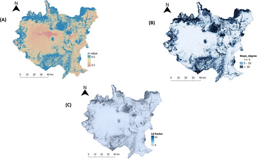
Where: λ is the horizontal projection of the slope length (m) = Flow Accumulation to each cell (FA*30m); θ is the slope (rad) = slope in degrees (°) x 0.01745. The length and slope of the standard USLE plot are 22.13 m and 0.0896 rad (5.14°), respectively; 'm‘ is a variable length-slope exponent ranging from 0.2 to 0.5. Figure 4 shows spatial distribution of the m-value, slope and the resulted LS factor.

Figure 4. Spatial distribution of length-slope exponent (a) m-value, (b) slope and (c) LS factor.

2.6.3. Soil erodibility (K-factor)

The RUSLE model’s K factor shows the vulnerability of soil erodibility related to soil characteristics (Wischmeier and Smith 1978). The factor reflects the cumulative effect of soil qualities such as soil texture, organic content, and sand, silt, and clay percentages (Renard et al. 1991). It denotes the susceptibility of soil or surface components to erosion as well as the transportability of silt.

The HWSD v1.2 soil database provides the above-mentioned field parameters for calculating K factor values for each soil type identified within the watershed (FAO Soil Portal 2019). The numbers were then loaded into the ArcGIS v.10.6 environments to generate a raster map of the K-factor value, which ranged between 0.141 and 0.17 t.ha.h.ha⁻¹.MJ⁻¹.mm⁻¹ (Figure 5).

Figure 5. Spatial distribution of major (a) soil types and their corresponding (b) K-factor values.

The calculation was performed based on William’s (1983) equation, Eq.7 as cited in Yan et al. (2018). (Eq.7) $$\mathrm{K}\mathrm{ }=f_{\mathit{csand}}\mathrm{*}{f}_{cl-si}\mathrm{*}{f}_{\mathrm{orgC}}\mathrm{*}{f}_{\mathit{hisand}}$$(Eq.7) where: $f_{\mathit{csand}}$ is a factor that lowers the K indicator in soils with a high proportion of coarse-sand content and higher for soils with little sand; $f_{cl-si}$ gives low soil erodibility factors for soils with a high clay-to-silt ratio; $f_{\mathrm{orgC}}$ reduces the K values in soils with a high organic carbon content while $f_{\mathit{hisand}}$ reduce the K value of soil classes with high sand contents. The $f_{\mathit{csand}},$ $\mathrm{ }{f}_{cl-si}\mathrm{ }{f}_{\mathrm{orgC}},$ and $f_{\mathit{hisand}}$ were calculated using Equation 8(Eq.8) $${\mathit{f}}_{\mathit{csand}}\mathrm{ }=(0.2+0.3.\mathrm{Exp}[-0256.\mathrm{ms}.\left(1+\frac{\mathrm{msilt}}{100}\right)\left]\right)$$(Eq.8) – Equation 11(Eq.11) $${\mathit{f}}_{\mathit{hisand}}\mathrm{ }=\left(1.0+\frac{0.7.(1-\frac{\mathrm{ms}}{100})}{\left(1-\frac{\mathrm{ms}}{100}\right)+\exp \left[5.51+22.9(1-\frac{\mathrm{ms}}{100})\right]}\right)$$(Eq.11) . (Eq.8) $${\mathit{f}}_{\mathit{csand}}\mathrm{ }=(0.2+0.3.\mathrm{Exp}[-0256.\mathrm{ms}.\left(1+\frac{\mathrm{msilt}}{100}\right)\left]\right)$$(Eq.8) (Eq.9) $${\mathit{f}}_{\mathit{cl}-\mathit{si}}\mathrm{ }={\left(\frac{\mathrm{msilt}}{\mathrm{mc}+\mathrm{msilt}}\right)}^{0.3}$$(Eq.9) (Eq.10) $${\mathit{f}}_{\mathbf{orgC}}=\left(1.0+\frac{0.256.\mathrm{orgC}}{\mathrm{orgC}+\exp \left[3.72-2.95.\mathrm{orgC}\right]}\right)$$(Eq.10) (Eq.11) $${\mathit{f}}_{\mathit{hisand}}\mathrm{ }=\left(1.0+\frac{0.7.(1-\frac{\mathrm{ms}}{100})}{\left(1-\frac{\mathrm{ms}}{100}\right)+\exp \left[5.51+22.9(1-\frac{\mathrm{ms}}{100})\right]}\right)$$(Eq.11) where: mc, ms, and msilt represent the percent (%) fraction of clay, sand, and silt, respectively. orgC is the soil organic carbon content (%).

2.6.4. Support practice (P-factor)

The support practice factor (P factor) or conservation practice refers to the conservation methods that lower the erosion potential of runoffs (Borrelli et al. 2017). Due to the difficulty of mapping the spatial difference of P-factor, many studies ignore it by assigning factor values of 1.0 over non- cultivated lands (Benavidez et al. 2018). In this case, the p-factor values can be estimated by combining slope percent and land use classifications (Wischmeier and Smith 1978). This study used the same values of p-factor values for estimating the soil loss during 1990-2000, 2000-2010 and 2010-2020, but accounting the spatial variation of LULC changes over time. This limitation represents one of the drawbacks of applying the RUSLE model for soil loss prediction. Nevertheless, the approach remain valid as minor changes of these factors are expected over the investigated periods (Benavidez et al. 2018).

Accordingly, the entire watershed was divided into cultivated and non-cultivated land regions, then superimposed with six slope classes (0-5%, 5-10%, 10-20%, 20-30%, 30-50%, and 50-100%). Based on literature reviews, the P-values were assigned for each slope class for the cultivated land and 0.8 to 1.0 for the non-cultivated land covers (Table 1). Finally, the two vector datasets were overlaid and rasterized using the spatial analyst tools in ArcGIS v10.6 Environment.

Table 1. LULC types and their corresponding P- factor and C- factor values.

LULC types	Slope (%)	P values	C values	References
Cultivated lands	0-5	0.1	0.15	(Wischmeier and Smith 1978; Hurni 1985; Bewket and Teferi 2009; Molla and Sisheber 2017; Yeneneh et al. 2022
	10-15	0.12
	15-20	0.14
	20-30	0.19
	30-50	0.25
	50-100	0.33
Bare lands	All slope class	1	0.6	(Haregeweyn et al. 2017; Molla and Sisheber 2017; Tsige et al. 2022; Belay and Mengistu 2021)
Built-up areas		0.8	0.09
Forest		0.8	0.01
Grazing lands		1	0.01
Shrubs		1	0.06
Water bodies		1	0

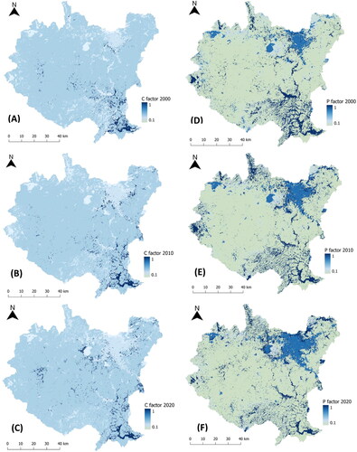
2.6.5. Cover management (C-factor)

The cover management (C-factor) determines the annual ratio of soil loss from LULC to bare lands. It indicates the impact of crops and other agricultural practices on erosion rates (Chalise et al. 2019). The C-factor represent spatiotemporal characteristics in response to the dynamics of vegetation and rainfall (Nearing et al. 2005). Similarly, both the cover and conservation management factors heavily influence the spatiotemporal dynamics of soil erosion in Ethiopia (Tamene et al. 2022). They do not normally change regularly due to the need of large-scale investments. Therefore, C-factor values were assigned from 0 to 0.6 to each LULC type following extensive literature reviews (Table 1). Figure 6 shows the spatial distribution of the P-factor and C-factor.

Figure 6. Spatial distribution of C-factor (a, b and c) and P-factor (d, e and f) values for the year 2000, 2010 and 2020, respectively.

2.7. Soil loss estimation

The RUSLE input factors (R, K, LS, C, and P factors) were implemented in a raster-based GIS environment to estimate mean annual soil loss for three consecutive decades (1990 – 2000, 2000 – 2010, and 2010 – 2020). These composite raster files were used for zonal statistical analysis in QGIS v.3.22.1 Processing Tools.

2.8. Zonal statistical analysis

Zonal statistical analysis was performed to explore the mean annual soil loss response to LULC and the corresponding transition matrix using image Processing Tools in QGIS v3.22.1. It generates data for area-weighted mean annual soil loss under each LULC type for three consecutive decades (1990-2000, 2000-2010, and 2010-2020). The analysis involves superimposing the composite thematic maps of the RUSLE model (i.e. spatial estimates of the mean annual soil loss) and LULC change and selected transition pathways.

3. Results

3.1. The LULC change

The LULC types determine the values of cover management (C-factor), which is the most sensitive spatiotemporal parameter of the RUSLE model (Nearing et al. 2005). Table 2 summarized descriptive statistics of the spatiotemporal analysis of the LULC schemes. The analysis revealed that cultivated land is the predominant land use type, represented by 81.6 − 85.9% of the total basin area between 1990 and 2020. Conversely, waterbodies, forests, grasslands, and bare land cover represented 0.2 − 3.3% of the total basin area during the same period. The spatial distribution of the classified LULC for each year is also presented in Figure 7. The overall classification accuracy of the thematic maps for 1990, 2000, 2010, and 2020 respectively achieved 76.3%, 79.4%, 85.7%, and 82.1%.

Figure 7. Spatial distribution of classified LULC for (a) 1990, (b) 2000, (c) 2010, and (d) 2020.

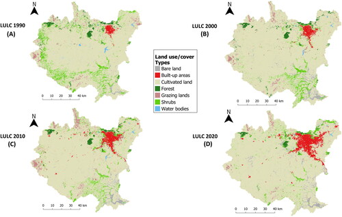
Table 2. Area coverage and proportion of LULC during 1990–2020.

LULC types	1990		2000		2010		2020
	km^2	%	km^2	%	km^2	%	km^2	%
Bare lands	71.6	0.9	175	2.24	209.5	2.68	256.8	3.3
Built-up areas	86.1	1.1	140.8	1.8	271.4	3.47	454.8	5.8
Cultivated land	6541.9	83.7	6709	85.9	6520.8	83.4	6381.1	81.6
Forest	247.4	3.2	225.9	2.3	145.1	1.9	98	1.3
Grassland	173.8	2.2	177.3	2.27	211.5	2.7	139.7	1.8
Shrubs	661.8	8.5	367.6	4.7	434.8	5.56	468.8	6
Water bodies	32.5	0.4	19.6	0.25	22	0.28	15.9	0.2

3.1.1. Annual rate of LULC change

The rate of LULC change varies over time. For example, cultivated land cover annually increased by 0.25% in the first decade (1990–2000) while decreasing by 0.28% and 0.22% during the second (2000–2010) and third decades (2010–2020), respectively (Figure 8). During the last three consecutive decades, bare land covers and built-up areas increased while forest cover decreased. Similarly, grassland cover sharply depleted at a rate of 4.15% in the third decade.

Figure 8. Standardized percent rate of annual LULC change.

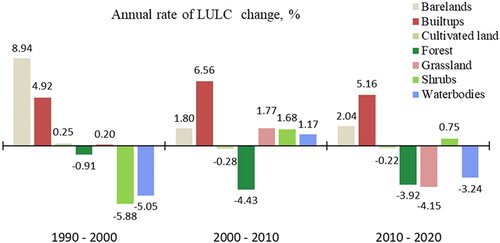
Although, the bare land covers relatively represents a small proportion of the basin area (0.9 − 3.3%), it increases at the fastest rate of 8.94% during the first decade. Consequently, it slows down by 1.8% and 2.04% during the last two decades, respectively. The rate of change of shrubs was also inconsistently varied over time. It decreases by 5.88% during the first decades, but slightly increases during the second and the third decades.

3.1.2. The LULC transition or conversion pathways

The LULC change experienced multiple ranges of conversion pathways during three consecutive decades. Appendix 3 shows each transition matrix and its corresponding spatial extents of the LULC. The result showed that the spatial gain of bare land, and cultivated land is greater as compared with its conversion from non-cultivated lands during the first decade. For example, the cultivated land cover increased by 2.5% (167 km²) during the first decade while decreased by 2.8% (188.1 km²) and 2.1% (139.7 km²) in the second and the third decades, respectively. It further, progressively encroaches a considerable extent of forest (142.2 km²), shrubs (780.8 km²), and grazing lands (274.5 km²). Conversely, the total area converted from forest, shrubs, and grasslands into cultivated land during these periods collectively comprised 611.3 km².

Summary of the LULC transition matrix (Table 3) reveals increased areas of cultivated land in the first decade (1990-2000), while decreasing in the last two decades (2000-2010 and 2010-2020). The increment coincides with decreased areas of forest and shrub landscapes, indicating encroachment of these landscapes. Conversely, the reduction in spatial extent coincides with increased extents of bare lands and built-up areas in the last two decades, presumably associated with urbanization, and competing demands of plantation woodlots over the cultivated lands. For example, Eucalyptus tree species is becoming a popular cash crop around farmlands in the basin.

Table 3. Area of gain, loss, and net changes (km²) of the major land cover schemes during 1990–2000, 2000–2010, and 2010–2020.

LULC schemes	1990–2000			2000–2010			2010–2020
	Gain	Loss	Net changes	Gain	Loss	Net changes	Gain	Loss	Net changes
Bare lands	135	31.6	103.4	119.4	84.9	34.5	156.5	109.2	47.3
Built-up areas	62	7.3	54.7	144.4	13.8	130.6	222.3	39	183.3
Cultivated land	658.6	491.6	167	372.1	560.2	−188.1	403.7	543.4	−139.7
Forest	90.5	112	−21.5	29.6	110.4	−80.8	17.8	64.9	−47.1
Grassland	97.7	94.2	3.5	117	82.8	34.2	53.8	125.6	−71.8
Shrubs	205.5	499.7	−294.2	286.6	219.4	67.2	268.2	234.2	34
Water bodies	7.5	20.4	−12.9	9.7	7.3	2.4	5.2	11.3	−6.1

3.1.3. Net gain or loss of LULC

Based on the transition matrix, Table 3 further summarized spatial extent of the gain or loss of each LULC scheme. Both forests and shrubs respectively lost an area of 21.5 km² and 294.2 km² during the first decade. Similarly, forest and cultivated lands respectively lost an area of 149.4 km² and 327.8 km² during the last three decades (1990-2020). Although the net loss of cultivated land outweighing the gain, it progressively encroaches a large extent of forest, shrubs, and grazing lands. The competing demand for urbanization and energy (fuel wood) may contribute for the loss of cultivated lands, which subsequently trigger grabbing of forest and shrub landscapes (Birhanu et al. 2021). For example, built-up areas and bare land cover progressively gained a spatial extent of 341.7 km² and 185.5 km² throughout the investigated periods of 1990 – 2020, which support the assumption. Similarly, an extensive net loss of forests, shrubs, grasslands, and water bodies occurred during the same periods.

3.2. Estimated mean annual soil loss

The spatial distribution of estimated soil loss during the last three consecutive decades (1990–2000, 2020–2010, and 2010–2020) is presented in Figure 9 (slight to severe). The estimated mean annual soil loss is 4.1 t/ha/y (0–138 t/ha/y), 4.4 t/ha/y (0–150 t/ha/y) and 5.1 t/ha/y (0–186 t/ha/y) during each consecutive decades, respectively. During the same period, the total annual soil loss is also estimated to be 3198.8 Mt/y, 3460.2 Mt/y, and 3985.7 Mt/y, respectively.

Figure 9. Spatial variability of the mean annual soil loss during (a) 1990–2000, (b) 2000–2010, and (c) 2010–2020.

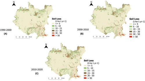
About 90% of the basin land area represents from slight to moderate erosion severity (< 10 t/ha/y) class. Similarly, 9.8% − 11.4% represent high to very severe (> 10 t/ha/y) vulnerability class (Table 4). During the last three decades, both the spatial extent and mean annual soil loss of very severe erosion class increased from 0.9% to 1.4% and from 87.4 t/ha/y to 110.3 t/ha/y, respectively.

Table 4. Soil loss severity class and spatial extent (km², %).

Range t/ha/y	Erosion severity class	Soil loss 2000			Soil loss 2010			Soil loss 2020
		km^2	%	Mean t/ha/y	km^2	%	Mean t/ha/y	km^2	%	Mean t/ha/y
0–5	Slight	6395.1	81.8	1.1	6397.6	81.9	1.1	6280.9	80.4	1.1
5–10	Moderate	655.3	8.4	7.1	612.3	7.8	7.1	647.2	8.3	7.1
10–15	High	270	3.5	12.1	255.7	3.3	12.2	279.3	3.6	12.2
15–30	Very high	319.8	4.1	21	337.7	4.3	21	365.1	4.7	21
30–50	Severe	105	1.3	38.2	121.7	1.6	38.1	131.3	1.7	38
>50	Very severe	69.9	0.9	87.4	90.1	1.2	94	111.3	1.4	110.3

3.2.1. Soil erosion response to LULC change

Different land use types cause different levels of soil loss severity. The mean annual soil loss is estimated to be 43.5, 49.9, and 56 t/ha/y in the 1^st, 2^nd and 3^rd decades, respectively (Table 5). Similarly, estimated soil loss from shrub land use schemes can be attributed to the high erosion severity class (10.1 – 14 t/ha/y). Both the mean and total annual soil loss over the bare landscapes progressively increased.

Table 5. Estimated rate of mean and total annual soil loss in response to LULC classes.

SN	LULC types	2000		2010		2020
		Mean loss t/ha/y	Total loss Mt/y*	Mean loss t/ha/y	Total loss Mt/y	Mean loss t/ha/y	Total loss Mt/y
1	Bare lands	43.5	761.9	49.9	1045.6	56	1438.9
2	Built-up areas	5.9	83.7	6.1	166.4	5.9	269.1
3	Cultivated lands	2.8	1886.7	2.4	1573.3	2.5	1566
4	Forest lands	3.5	79.2	3.3	48.3	3.6	34.9
5	Grasslands	0.9	15.9	1.1	24.1	1	14.7
6	Shrub lands	10.1	371.4	13.9	602.5	14.1	662.1

*Mt/y refers to metric tons per year.

Similarly, cultivated land cover exhibits a very slight amount of mean annual soil loss (2.4 − 2.8 t/ha/y) as the area reduced with time while the percent contribution to the total annual soil loss is considerably high (39.3% − 59%).

3.2.2. Soil erosion response to LULC transition matrix

Soil loss estimate with reference to land use and cover transition is crucial in the decision-making process of watershed management. Unlike the conventional approach, this particular study evaluated soil loss severity in response to land use conversion pathways. Table 6 illustrates zonal statistical analysis of mean annual soil loss for some LULC conversion pathways (from-to), which represents high to very severe erosivity class. The estimated mean annual soil loss for those pathways, which represent the loss above tolerable limit. The estimated soil loss widely ranges from 26.7 − 107.1 t/ha/y, 28.8 – 82 t/ha/y, and 41 – 136 t/ha/y, during the three consecutive decades, respectively.

Table 6. Ranked estimates of soil loss response to LULC change transitions (from-to).

From 1990-2000	Mean loss t/ha/y	From 2000-2010	Mean loss t/ha/y	From 2010-2020	Mean loss t/ha/y
7-1	107.1	7-1	82	4-1	136
4-1	83.4	2-1	67.2	5-1	127.4
6-1	64.9	6-1	59.7	7-1	87.6
2-1	56.4	4-1	58	6-1	83
1 (Unchanged)	46	3-1	50.8	3-1	55.2
3-1	40	1 (Unchanged)	46.7	1 (Unchanged)	54.9
5-1	26.7	5-1	28.8	2-1	41
4-6	15.7	4-6	21.2	4-6	18.5
4-2	14.9	7-6	16.8	7-5	16.7
4-3	13.1	4-2	13.6	4-2	14.8
6 (Unchanged)	11.1	3-6	13.2	4-3	12.5
		5-6	12.4	6-5	11.5
		6 (Unchanged)	12.2

1 = Bare land; 2 = Built-up areas; 3 = Cultivated land; 4 = Forest; 5 = Grassland; 6 = Shrubs; 7 = Water bodies.

4. Discussion

Understanding the LULC dynamics in a given watershed requires thematic maps of multi-temporal LULCs produced by using a robust classification procedure. Unlike the conventional approach, this particular study further examined the spatiotemporal dynamics of LULCs. As a result, the classified thematic maps of 1990, 2000, 2010 and 2020 used in optimizing interpretations of the soil erosion severity in the basin. Accordingly, their overall classification accuracy range from 79.4% to 85.7%, which reveals a high level of agreement between the classified maps and the referenced data (Congalton and Green 2019). Cultivated land cover is the dominant form of LULC in upper Awash River Basin, which was also reported by previous studies (Shawul and Chakma 2019; Alem 2022)

4.1. Spatiotemporal dynamics of LULCs

Results from the analysis of annual rate of change further revealed progressively encroach and deplete protective land covers, like forests. Similarly, the shrubs, bare lands, and cultivated land covers showed varying rate of change over the years. For example, the cultivated land in the first decade (1990-2000) is most likely expanding on cost of shrubs and forest cover. A similar study on spatiotemporal dynamics of land use/cover in the Blue Nile basin has revealed consistent expansion of cultivated land at the expense of forest covers (Yesuph and Dagnew 2019).

Moreover, the high competing demand for non-agricultural land uses in the recent decades, particularly for built-up areas, would likely continue because of the increasing population pressure in the basin (Birhanu et al. 2021). Consequently, the demand for agricultural lands would increase. This would rather triggers farmers to cultivate marginal and fragile landscapes. The results confirm this assumption. For example, the annual rate of bare land expansion decreases from 8.94% in the first decades to 1.8% and 2.04% respectively in the second and third decades. The reason for such sharply declining rate of expansion during the last two decades may be that farmers presumably compelled to use the bare landscapes for cultivating agricultural crops. For example, more than half of the bare land cover was grabbed for cultivation purpose (Appendix 3).

Similarly, during the last two decades cultivated land covers alarmingly encroached, and thus resulted a net loss of spatial extent. This is mainly due to the expansion of bare lands and built-up areas. Such aggressive expansion of non-agricultural lands further encroaches the cultivated lands, which inevitably push farmers to cultivate marginal and most fragile landscapes (Yesuph and Dagnew 2019). Nevertheless, cultivating vulnerable landscapes without proper conservation measures could have substantial negative impacts on soil erosion (Meng et al. 2021; Masroor et al. 2022). Soil erosion severity often attributed with increasing expansion of agricultural lands (Bekele 2019; Kidane et al. 2019; Negese 2021; Alem 2022). In this particular study, however, the decreasing extent of cultivated land does not necessarily implies reduced level of soil erosivity. The net loss of cultivated land cover exceeds the gain, while it progressively encroaching over a large extent of protective land covers such as forest, shrubs, and grazing lands. However, the rate of annual loss is slower than the rate of encroachment over these protective land covers. Several studies in Ethiopia reported increased expansion of cultivated land (references). Unlike these reports, it is steadily decreasing in upper Awash River basin. For example, regarding the overall estimates of mean annual soil loss from cultivated land, the severity looks slight while contributing the largest proportion to total annual soil loss. Thus, without closely interpreting the dynamics of LULC, the decreasing extent of the cultivated land could mislead decision making on conservation planning.

The results also showed that conversion of LULC into bare landscapes (abandoned and left without any treatment) accelerates soil erosion. Studies also indicated that conversion of LULC determines the rate of soil loss (Bekele 2019; Negese 2021; Teshome et al. 2022). For example, regardless of land use practices, conversion from waterbodies, grassland, shrubs and forests into bare land cover may causes severe soil erosion (up to 136 t/ha/year). This is again because of the high rate of erodibility of bare soils (Masroor et al. 2022). Despite the spatial extent of bare land cover relatively accounts smaller proportion of the basin area, it represents a severe erosion hazard (up to 56 t/ha/y). Unless appropriate conservation measures are implemented, these particular pathways may increase the prevailing soil erosion process in the upper Awash River basin. The conversion pathways may be influenced by a variety of factors other than changes in the land use/cover of the basin (Bekele et al. 2017), and hence further research is needed to fully understand these trends and their implications.

4.2. Response of mean annual soil loss to LULCs

Zonal statistical analysis of LULC change revealed noticeable variations in the soil loss responses. The analysis further revealed that the bare landscapes are the most vulnerable type of land cover schemes. However, interpreting the mean annual soil loss alone does not accurately represent the level of severity. Regarding the impacts of LULC change on soil erosion and hydrological responses, analysis of the LULC transition matrix confirmed prior studies conducted in Ethiopia, For example, the average rate of soil erosion, sediment output, and surface runoff increases during the last four decades, mainly due to cultivated lands expansion at the expense of forestlands, shrubs, and grasslands (Bekele 2019; Negese 2021). Thus, optimal interpretation of soil erosion estimates rather requires a detailed analysis of the net gain or loss of LULC schemes for making informed decision on conservation priority.

With a closer visual interpretation of the RUSLE model output (spatial variability of mean annual soil loss), the downstream areas of the watershed represents very severe soil loss potential despite slope gradient is relatively lower. This is mainly because of the influence of LULC type, which is dominantly represented by bare landscapes. Essentially, the downstream region deserves special attention as critical watershed features such rivers, lakes, wetlands, and gully channels are located. They are often threatened by flood damage and other environmental calamities. For example, a study showed that one billion tons of suspended sediment enter rivers each year as a result of human-caused soil erosion (Hurni et al. 2015). Such deposition of sediment into river channels, particularly in the upper Awash River basin, inevitably resulting catastrophic flood damage on nearby farmlands (FloodList News 2020). Apart from the mean annual soil loss values, any soil conservation priority would have much greater benefits in mitigating the potential soil erosion risk.

4.3. Limitations of the study

Although the RUSLE model is one of the widely used empirical models for predicting potential soil erosion, it tends to overestimate soil loss across a wider range of slopes and diverse landscapes. It also represents only the rill and inter-rill soil erosion process, excluding mass and gully erosion processes. In addition to these inherited limitations, it may also be argued that the model does not account for temporal fluctuations of C and P factors in this particular study. Because it is not feasible to monitor these parameters at the watershed scale, the model promptly used the same values with response to the LULC change over time. Similarly, the rainfall erosivity (R factor) was indirectly derived from regression model, which had been recommended for soil erosion assessment in the Ethiopian highlands since 1985. It is likely obsoleted due to the dynamic nature of land use/cover and climate change. Despite these limitations, the study has attempted to optimize uncertainty of the model output through zonal statistical analysis of soil erosion response to the annual rate of land cover change, net gain or loss, and the transition matrix. This approach could help to portray the severity of soil erosion risk in the study area.

5. Conclusion and recommendations

This study demonstrates how to optimize interpreting soil erosion estimates through a detailed analysis of LULC change. It also highlights the need to carefully interpret model results in future studies. Utilizing the RUSLE model to determine conservation priorities is not ideal due to inherited mathematical faults. This is especially true where gully erosion is a predominant form of soil erosion in a watershed like the study area. Thus, interpreting the response of soil erosion in a watershed could be improved with further investigation of land use and cover changes. Thus, to prevent further degradation of protective land covers, continued monitoring, and management of the basin area is indispensable. This particular study, in general, highlights the need for interpreting soil erosion vulnerability beyond the magnitude of the RUSLE-based mean annual soil loss values, which otherwise misleads our decision on conservation priority. Similar future research should adhere to this approach while interpreting the results.

Data availability statement

The datasets and materials supporting the results or analyses presented in this paper are available upon request.

Disclosure statement

No potential conflict of interest was reported by the authors.

Additional information

Funding

This study was funded by the World Bank Group, through Africa Center of Excellence for Climate Smart Agriculture and Biodiversity Conservation, Haramaya University (Ethiopia).

Appendices

 

Appendix 2. Imputation of missing daily rainfall values for weather stations (samples).

Appendix 1. Information of weather stations and mean annual rainfall recorded from 1987 to 2020

SN	Weather Stations	Latitude	Longitude	Elevation (meter)	MARF*, mm
1	Alem Tena	8.29	38.91	1656	822.6
2	Ambo	8.98	37.84	2068	1029.3
3	Asgori	8.79	38.33	2072	1031.4
4	Bantuliben	8.62	38.36	2167	1075.3
5	Boneya	8.78	38.64	2251	928.6
6	Bui	8.33	38.55	2054	1045.7
7	Chefedonsa	8.97	39.12	2392	898.6
8	Hombole	8.37	38.77	1743	739.6
9	Jeldu	9.25	38.08	2952	1558
10	Kimoye	9.01	38.34	2150	1038.3
11	Koka Dam	8.5	39.15	1618	925
12	Lemen	8.6	38.61	2082	906.5

* MARF = Mean annual rainfall

Appendix 3. Transition matrix of spatiotemporal LULC during (a) the 1^st decade (1990–2000); (b) the 2^nd decade (2000–2010); and (c) the 3^rd decade (2010–2020).

1^st decade	LULC 2000 (in km^2)
LULC 1990	Bare lands	Built-up areas	Cultivated land	Forest	Grassland	Shrubs	Water bodies	Total
Bare lands	40	0.8	25.9	0	0	4.7	0.2	71.6
Built-up areas	0.4	78.8	4.7	0.1	0	1	1.1	86.1
Cultivated land	120.6	57.9	6050.3	40.6	90.2	177.9	4.4	6541.9
Forest	0	1.2	88.7	135.4	1.3	20.2	0.6	247.4
Grassland	0.1	0.1	92.3	0.8	79.6	0.8	0	173.8
Shrubs	13.3	1.4	430.3	48.4	5.1	162.1	1.3	661.8
Water bodies	0.6	0.6	16.8	0.5	1	1	12.1	32.5
Total	175	140.8	6708.9	225.9	177.3	367.6	19.6	7815.1
2^nd decade	LULC 2010 (in km^2)
LULC 2000	Bare lands	Built-up areas	Cultivated land	Forest	Grassland	Shrubs	Water bodies	Total
Bare lands	90.1	9.5	72.4	0	0.5	2.1	0.4	175
Built-up areas	2.9	127	7.2	0.2	0.2	3.1	0.2	140.8
Cultivated land	99.4	108.6	6148.7	19.3	109.1	216.4	7.4	6708.9
Forest	0.1	5.5	43.7	115.5	3.7	57.2	0.1	225.9
Grassland	1	1.5	72.6	0.5	94.5	6.9	0.3	177.3
Shrubs	15.1	17.5	172.5	9.4	3.5	148.2	1.3	367.6
Water bodies	0.7	1.9	3.6	0.1	0.1	0.9	12.3	19.6
Total	209.5	271.4	6520.8	145.1	211.5	434.8	22	7815.1
3^rd decade	LULC 2020 (in km^2)
LULC 2010	Bare lands	Built-up areas	Cultivated land	Forest	Grassland	Shrubs	Water bodies	Total
Bare lands	100.3	33	74.7	0	0.2	0.9	0.4	209.5
Built-up areas	4.4	232.4	23.8	0.7	0.2	9.6	0.2	271.4
Cultivated land	143.6	150.3	5977.4	5	47.3	193.4	3.8	6520.8
Forest	0.3	2	9.8	80.2	0.7	51.8	0.2	145.1
Grassland	1.3	2.6	109.6	0.5	85.9	11.6	0	211.5
Shrubs	6.1	32.9	178	11.5	5.1	200.6	0.7	434.8
Water bodies	0.8	1.6	7.8	0	0.2	0.9	10.7	22
Total	256.8	454.7	6381.1	98	139.7	468.8	15.9	7815.1

Appendix 4. Description of LULC schemes.

ID	Land use/ cover Types	Description
1	Bare lands	Landscapes with bare soil, unused for a longer period, are often left abandoned landscape without any treatments and result in further degradation
2	Built-up areas	paved surface, buildings of residential and commercial, transportation routes etc
3	Cultivated land	any agricultural lands crop fields and fallow lands used for rainfed and irrigated agriculture, including homestead farmlands
4	Forest	continuous stand of trees with closed canopy cover, mostly grown over mountainous areas as natural forest and as a patch of riverine forest along streams
5	Grassland	landscape mainly used for grazing lands
6	Shrubs	landscapes covered with sparse vegetation, fragmented patches of trees grown as woodlots near farmlands or homestead areas
7	Water bodies	any water bodies including rivers, lakes, ponds, wetlands etc

References

- Abdul Rahaman S, Aruchamy S, Jegankumar R, Abdul Ajeez S. 2015. Estimation of annual average soil loss, based on rusle model in Kallar Watershed, Bhavani Basin, Tamil Nadu. ISPRS Ann Photogramm Remote Sens Spatial Inf Sci. II-2/W2:207–214. doi: 10.5194/isprsannals-II-2-W2-207-2015.
- Abebe BA, Grum B, Degu AM, Goitom H. 2022. Spatio-temporal rainfall variability and trend analysis in the Tekeze-Atbara river basin, northwestern Ethiopia. Meteorol Appl. 29(2):1–17. doi: 10.1002/met.2059.
- Alem BB. 2022. The nexus between land use land cover dynamics and soil erosion hotspot area of Girana Watershed, Awash Basin, Ethiopia. Heliyon. 8(2):e08916. doi: 10.1016/J.HELIYON.2022.E08916.
- Bailey BE, Andridge R, Shoben AB. 2020. Multiple imputation by predictive mean matching in cluster-randomized trials. BMC Med Res Methodol. 20(1):72. doi: 10.1186/s12874-020-00948-6.
- Batar AK, Watanabe T, Kumar A. 2017. Assessment of land-use/land-cover change and forest fragmentation in the Garhwal Himalayan Region of India. Environments. 4(2):34. doi: 10.3390/environments4020034.
- Bekele D, Alamirew T, Kebede A, Zeleke G, Melese AM. 2017. Analysis of rainfall trend and variability for agricultural water management in Awash River Basin, Ethiopia. J Water and Climate Change. 8(1):127–141. doi: 10.2166/wcc.2016.044.
- Bekele T. 2019. Effect of land use and land cover changes on soil erosion in Ethiopia. Int J Agric Sc Food Technol. 5(1):26–34. doi: 10.17352/2455-815X.000038.
- Belay T, Mengistu DA. 2021. Impacts of land use/land cover and climate changes on soil erosion in Muga watershed, Upper Blue Nile basin (Abay), Ethiopia. Ecol Process. 10(1):1–23. doi: 10.1186/s13717-021-00339-9.
- Benavidez R, Jackson B, Maxwell D, Norton K. 2018. A review of the (Revised) Universal Soil Loss Equation ((R)USLE): with a view to increasing its global applicability and improving soil loss estimates. Hydrol Earth Syst Sci. 22(11):6059–6086. doi: 10.5194/hess-22-6059-2018.
- Bewket W, Teferi E. 2009. Assessment of soil erosion hazard and prioritization for treatment at the watershed level: Case study in the Chemoga watershed, Blue Nile basin, Ethiopia. Land Degrad Dev. 20(6):609–622. doi: 10.1002/ldr.944.
- BirdLife International. 2022. Important Bird Areas factsheet: Koka dam and Lake Gelila. http://datazone.birdlife.org/site/factsheet/koka-dam-and-lake-gelila-iba-ethiopia.
- Birhanu B, Kebede S, Charles K, Taye M, Atlaw A, Birhane M. 2021. Impact of natural and anthropogenic stresses on surface and groundwater supply sources of the upper Awash Sub-Basin, Central Ethiopia. Front Earth Sci. 9:656726. doi: 10.3389/feart.2021.656726.
- Borrelli P, Robinson DA, Fleischer LR, Lugato E, Ballabio C, Alewell C, Meusburger K, Modugno S, Schütt B, Ferro V, et al. 2017. An assessment of the global impact of 21st century land use change on soil erosion. Nat Commun. 8(1):2013. doi: 10.1038/s41467-017-02142-7.
- Breiby T. 2006. Assessment of soil erosion risk within a subwatershed using GIS and RUSLE with a comparative analysis of the use of STATSGO and SSURGO soil databases. Papers in Resource Analysis. Winona, MN: Saint Mary’s University of Minnesota Central Services Press. https://gis.smumn.edu/GradProjects/BreibyT.pdf.
- Bussi G, Whitehead PG, Jin L, Taye MT, Dyer E, Hirpa FA, Yimer YA, Charles KJ. 2021. Impacts of climate change and population growth on river nutrient loads in a data scarce region: the Upper Awash River (Ethiopia). Sustainability (Switzerland). 13(3):1254. doi: 10.3390/su13031254.
- Central Statistical Agency (CSA). 2014. Population Projection of Ethiopia for All Regions At Wereda Level from 2014 – 2017. Addis Ababa, Ethiopa: Federal Demographic Republic of Ethiopia Central Statistical Agency. http://www.statsethiopia.gov.et/population-projection/.
- Chalise D, Kumar L, Kristiansen P. 2019. Land degradation by soil erosion in Nepal: a review. Soil Syst. 3(1):12. doi: 10.3390/soilsystems3010012.
- Congalton RG, Green K. 2019. Assessing the accuracy of remotely sensed data principles and practices. Boca Raton, FL: y Taylor & Francis Group, LLC.
- Dawit M, Halefom A, Teshome A, Sisay E, Shewayirga B, Dananto M. 2019. Changes and variability of precipitation and temperature in the Guna Tana watershed, Upper Blue Nile Basin, Ethiopia. Model Earth Syst Environ. 5(4):1395–1404. doi: 10.1007/S40808-019-00598-8/METRICS.
- FAO Soil Portal. 2019. Harmonized world soil database v1.2 | FAO SOILS PORTAL | Food and Agriculture Organization of the United Nations, Rome. https://www.fao.org/soils-portal/data-hub/soil-maps-and-databases/harmonized-world-soil-database-v12/en/.
- FloodList News. 2020. Ethiopia – 144,000 Displaced by Awash River Flooding in Afar Region – FloodList. https://floodlist.com/africa/-ethiopia-floods-afar-september-2020.
- Ganasri BP, Ramesh H. 2016. Assessment of soil erosion by RUSLE model using remote sensing and GIS - A case study of Nethravathi Basin. Geosci Front. 7(6):953–961. doi: 10.1016/j.gsf.2015.10.007.
- Gebremichael HB, Raba GA, Beketie KT, Feyisa GL, Siyoum T. 2022. Changes in daily rainfall and temperature extremes of upper Awash Basin, Ethiopia. Sci Afr. 16:e01173. doi: 10.1016/j.sciaf.2022.e01173.
- Gebreselassie S, Kirui OK, Mirzabaev A. 2015. Economics of land degradation and improvement in Ethiopia. In: Nkonya E, Mirzabaev A, von Braun J editors. Economics of land degradation and improvement - A global assessment for sustainable development; Cham: Springer; p. 401–430. doi: 10.1007/978-3-319-19168-3_14/TABLES/18.
- Gelagay HS, Minale AS. 2016. Soil loss estimation using GIS and Remote sensing techniques: a case of Koga watershed, Northwestern Ethiopia. Int Soil and Water Conserv Res. 4(2):126–136. doi: 10.1016/j.iswcr.2016.01.002.
- Getachew B, Manjunatha BR, Bhat GH. 2021. Assessing current and projected soil loss under changing land use and climate using RUSLE with Remote sensing and GIS in the Lake Tana Basin, Upper Blue Nile River Basin, Ethiopia. Egyptian J Remote Sensing and Space Sci. 24(3):907–918. doi: 10.1016/j.ejrs.2021.10.001.
- Girma T, Sonder K, Peden D. 2015. The water of the Awash River basin a future challenge to Ethiopia. https://www.researchgate.net/publication/265483628.
- Halcrow. 1989. Master plan for the development of surface water resources in the Awash Basin. Final Report Vol.5, Annex C Assessment of Groundwater Potential. Addis Ababa: Ethiopian Valleys Development Authority, Irrigation and Drainage.
- Haregeweyn N, Tsunekawa A, Poesen J, Tsubo M, Meshesha DT, Fenta AA, Nyssen J, Adgo E. 2017. Comprehensive assessment of soil erosion risk for better land use planning in river basins: Case study of the Upper Blue Nile River. Sci Total Environ. 574:95–108. doi: 10.1016/j.scitotenv.2016.09.019. 27623531
- Honningsvag B, Midttomme GH, Repp K, Vaskinn K, Westeren T. editors. 2001. Hydropower in the new millennium. Proceedings of the 4th International Conference Hydropower; June 20–22, Bergen, Norway. London: CRC Press. https://doi.org/10.1201/9781003078722.
- Hurni H. 1985. Soil conservation manual for Ethiopia : a field guide for conservation implementation. Publisher: Verlag nicht ermittelbar, Addis Abeba. WorldCat.org.
- Hurni K, Zeleke G, Kassie M, Tegegne B, Kassawmar T, Teferi E, Amdihun A, Mekuriaw A, Debele B, Deichert G, and Hurni H., 2015. Economics of Land Degradation (ELD) Ethiopia Case Study. Soil Degradation and SustainableLand Management in the Rainfed Agricultural Areas of Ethiopia: An Assessment of the EconomicImplications. Report for the Economics of Land Degradation Initiative. 94 pp. Bonn, Germany. Available at www.eld-initiative.org
- Hurni. 1988. Degradation and conservation of the resources in the Ethiopian highlands. Mt Res Dev. 8:123–130. doi: 10.2307/3673438.
- Kidane M, Bezie A, Kesete N, Tolessa T. 2019. The impact of land use and land cover (LULC) dynamics on soil erosion and sediment yield in Ethiopia. Heliyon. 5(12):e02981. doi: 10.1016/j.heliyon.2019.e02981.
- Luca C. 2021. Semi-automatic classification plugin—QGIS python plugins repository. https://plugins.qgis.org/plugins.
- Masroor M, Sajjad H, Rehman S, Singh R, Hibjur Rahaman M, Sahana M, Ahmed R, Avtar R. 2022. Analysing the relationship between drought and soil erosion using vegetation health index and RUSLE models in Godavari middle sub-basin, India. Geosci Front. 13(2):101312. doi: 10.1016/j.gsf.2021.101312.
- Meng X, Zhu Y, Yin M, Liu D. 2021. The impact of land use and rainfall patterns on the soil loss of the hillslope. Sci Rep. 11(1):16341. doi: 10.1038/s41598-021-95819-5.
- Mohamed MA, El Afandi GS, El-Mahdy MES. 2022. Impact of climate change on rainfall variability in the Blue Nile basin. Alexandria Engin J. 61(4):3265–3275. doi: 10.1016/j.aej.2021.08.056.
- Molla T, Sisheber B. 2017. Estimating soil erosion risk and evaluating erosion control measures for soil conservation planning at Koga watershed in the highlands of Ethiopia. Solid Earth. 8(1):13–25. doi: 10.5194/se-8-13-2017.
- Moore ID, Wilson JP. 1992. Length-slope factors for the Revised Universal Soil Loss Equation: Simplified method of estimation. J Soil Water Conserv. 47(5):423–428.
- Moritz S, Bartz-Beielstein T. 2017. imputeTS: time Series missing value imputation in R. R J. 9(1):207. doi: 10.32614/RJ-2017-009.
- Nearing MA, Jetten V, Baffaut C, Cerdan O, Couturier A, Hernandez M, Le Bissonnais Y, Nichols MH, Nunes JP, Renschler CS, et al. 2005. Modeling response of soil erosion and runoff to changes in precipitation and cover. Catena (Amst). 61(2–3):131–154. doi: 10.1016/j.catena.2005.03.007.
- Negese A. 2021. Impacts of land use and land cover change on soil erosion and hydrological responses in Ethiopia. Appl Environ Soil Sci. 2021:1–10. doi: 10.1155/2021/6669438.
- Olofsson P, Foody GM, Herold M, Stehman SV, Woodcock CE, Wulder MA. 2014. Good practices for estimating area and assessing accuracy of land change. Remote Sens Environ. 148:42–57. doi: 10.1016/j.rse.2014.02.015.
- Pandey S, Kumar P, Zlatic M, Nautiyal R, Panwar VP. 2021. Recent advances in assessment of soil erosion vulnerability in a watershed. Int Soil Water Conserv Res. 9(3):305–318. doi: 10.1016/j.iswcr.2021.03.001.
- Pham TG, Degener J, Kappas M. 2018. Integrated universal soil loss equation (USLE) and Geographical Information System (GIS) for soil erosion estimation in A Sap basin: Central Vietnam. Int Soil and Water Conserv Res. 6(2):99–110. doi: 10.1016/j.iswcr.2018.01.001.
- Puyravaud JP. 2003. Standardizing the calculation of the annual rate of deforestation. For Ecol Manage. 177(1–3):593–596. doi: 10.1016/S0378-1127(02)00335-3.
- Renard KG, Foster GR, Weesies GA, Porter JP. 1991. RUSLE: revised universal soil loss equation. J Soil Water Conserv. 46:30–33.
- Sabr A, Moeinaddini M, Azarnivand H, Guinot B. 2016. Assessment of land use and land cover change using spatiotemporal analysis of landscape: case study in south of Tehran. Environ Monit Assess. 188(12):691. doi: 10.1007/S10661-016-5701-9/METRICS.
- Sarkar S, Kanungo DP, Mehrotra GS. 1995. Landslide hazard zonation: a case study in Garhwal Himalaya, India. Mt Res Dev. 15(4):301–309. doi: 10.2307/3673806.
- Shawul AA, Chakma S. 2019. Spatiotemporal detection of land use/land cover change in the large basin using integrated approaches of remote sensing and GIS in the Upper Awash basin, Ethiopia. Environ Earth Sci. 78(5):141. doi: 10.1007/s12665-019-8154-y.
- Shawul AA, Chakma S. 2020. Trend of extreme precipitation indices and analysis of long-term climate variability in the Upper Awash basin, Ethiopia. Theor Appl Climatol. 140(1–2):635–652. doi: 10.1007/s00704-020-03112-8.
- Shi P, Castaldi F, van Wesemael B, Van Oost K. 2020. Vis-NIR spectroscopic assessment of soil aggregate stability and aggregate size distribution in the Belgian Loam Belt. Geoderma. 357:113958. doi: 10.1016/j.geoderma.2019.113958.
- Shisanya CA, Recha C, Anyamba A. 2011. Rainfall variability and its impact on normalized difference vegetation index in arid and semi-arid lands of Kenya. IJG. 2(1):36–47. doi: 10.4236/ijg.2011.21004.
- Tadesse A, Dai W. 2019. Prediction of sedimentation in reservoirs by combining catchment based model and stream based model with limited data. Int J Sediment Res. 34(1):27–37. doi: 10.1016/j.ijsrc.2018.08.001.
- Tamene L, Abera W, Demissie B, Desta G, Woldearegay K, Mekonnen K. 2022. Soil erosion assessment in Ethiopia: a review. J Soil Water Conserv. 77(2):144–157. doi: 10.2489/jswc.2022.00002.
- Teshome A, Zhang J. 2019. Increase of extreme drought over Ethiopia under climate warming. Adv Meteorol. 2019:1–18. doi: 10.1155/2019/5235429.
- Teshome DS, Moisa MB, Gemeda DO, You S. 2022. Effect of land use-land cover change on soil erosion and sediment yield in muger sub-basin, Upper Blue Nile Basin, Ethiopia. Land (Basel). 11(12):2173. doi: 10.3390/land11122173.
- Tessema N, Kebede A, Yadeta D. 2020. Modeling land use dynamics in the Kesem sub-basin, Awash River basin, Ethiopia. Cogent Environ Sci. 6(1):1782006. doi: 10.1080/23311843.2020.1782006.
- Tsige MG, Malcherek A, Seleshi Y. 2022. Estimating the best exponent and the best combination of the exponent and topographic factor of the modified Universal soil loss equation under the hydro-climatic conditions of ethiopia. Water. 14(9):1501.doi: 10.3390/w14091501.
- Verstraeten G, Poesen J, Demarée G, Salles C. 2006. Long-term (105 years) variability in rain erosivity as derived from 10-min rainfall depth data for Ukkel (Brussels, Belgium): Implications for assessing soil erosion rates. J Geophys Res. 111(D22):1–19. doi: 10.1029/2006JD007169.
- Vivid Economics. 2016. Water resources and extreme events in the Awash basin: economic effects and policy implications. London, United Kingdom: Report prepared for the Global Green Growth Institute.
- Wang M, An Z, Wang S. 2022. The time lag effect improves prediction of the effects of climate change on vegetation growth in Southwest China. Remote Sens (Basel). 14(21):5580. doi: 10.3390/rs14215580.
- Wischmeier WH, Smith DD. 1978. Predicting rainfall erosion losses. In: A guide to conservation planning. The USDA Agricultural Handbook No. 537. MD: Scientific Research Publishing.
- World Bank. 2007. The cost of land degradation in Ethiopia : a review of past studies. Washington, DC. http://hdl.handle.net/10986/7939.
- Yan R, Zhang X, Yan S, Chen H. 2018. Estimating soil erosion response to land use/cover change in a catchment of the Loess Plateau, China. Int Soil and Water Conserv Res. 6(1):13–22. doi: 10.1016/j.iswcr.2017.12.002.
- Yeneneh N, Elias E, Feyisa GL. 2022. Quantify soil erosion and sediment export in response to land use/cover change in the Suha watershed, northwestern highlands of Ethiopia: Implications for watershed management. Environ Sci Res. 11(1):1–19. doi: 10.1186/S40068-022-00265-5.
- Yesuf M, Mekonnen A, Kassie M, Pender J, Kohlin G, Bojö J, Lutz E, Margulis S, Loening J, Pagiola S. 2005. Cost of land degradation in Ethiopia: A critical review of past studies. Environmetnal economics policy forum for Ethiopia (EEPFE). https://www.efdinitiative.org/sites/default/files/cost_land_degradation.pdf.
- Yesuph AY, Dagnew AB. 2019. Land use/cover spatiotemporal dynamics, driving forces and implications at the Beshillo catchment of the Blue Nile Basin, North Eastern Highlands of Ethiopia. Environ Syst Res. 8(1):1–30. doi: 10.1186/s40068-019-0148-y.
- Zerkani S, Abba EH, Zerkan H, Zair T, Zine N-E. 2022. The impact of the precipitation on the vegetation and ecological quality in the River of Oued Guigou, Morocco. IOP Conf Ser: Earth Environ Sci. 1090(1):012036. doi: 10.1088/1755-1315/1090/1/012036.