Random forest-based multi-hazard loss estimation using hypothetical data at seismic and tsunami monitoring networks

Abstract

This article presents a novel approach to estimate multi-hazard loss in a post-event situation, resulting from cascading earthquake and tsunami events with machine learning for the first time. The proposed methodology combines the power of random forest (RF) with data that are simulated at seismic and tsunami monitoring locations. The RF model is well-suited for predicting highly nonlinear multi-hazard loss because of its nonparametric regression and ensemble learning capabilities. The study targets the cities of Iwanuma and Onagawa in Tohoku, Japan, where seismic and tsunami monitoring networks have been deployed. To encompass a diverse range of future multi-hazard loss estimation, an RF model is constructed based on 4000 simulated earthquake events with peak ground velocity and tsunami wave amplitude captured at ground-motion monitoring sites and offshore wave monitoring sensors, respectively. The incorporation of 10 ground-motion monitoring sites and five offshore wave monitoring sensors significantly enhances the model’s forecasting power, leading to a notable 60% decrease in mean squared error and 20% increase in the $R^2$ value compared to scenarios where no monitoring sensors are utilized. By harnessing the capabilities of RF and leveraging detailed sensing data, RF achieves $R^2$ values over 90%, which can contribute to enhanced disaster risk management.

Keywords:

• Multi-hazard loss
• random forest
• subduction zone
• coastal communities
• monitoring sensors

1. Introduction

Severe damage caused by earthquakes and tsunamis has been well-documented in numerous historical events, highlighting their devastating impacts to coastal regions. The 2011 Great East Japan earthquake and tsunami, for example, resulted in widespread destruction and long-term socio-economic impacts in the Tohoku region of Japan (Mori et al. 2012). Similarly, the 2004 Indian Ocean earthquake and tsunami led to catastrophic consequences across multiple countries, causing significant casualties and extensive damage to infrastructure (Jaffe et al. 2006). These events serve as stark reminders of the destructive power of seismic and tsunami events, emphasizing the importance of accurate estimation of multi-hazard losses (e.g. direct economic loss from damage of building assets) to inform effective disaster risk reduction strategies.

Effective recovery and risk mitigation efforts in coastal regions require accurate estimation of the potential losses associated with these events. There are existing systems for earthquake loss estimation, such as the United States Geological Survey’s PAGER (Prompt Assessment of Global Earthquakes for Response) (Jaiswal et al. 2010). Besides, other research groups have focused on the rapid impact and loss estimation of earthquakes (Erdik et al. 2011; Ranjbar et al. 2017; Elkady et al. 2020; Scheingraber and Käser 2020; Yalcin et al. 2020) and tsunamis (Benchekroun et al. 2015; Virtriana et al. 2023). These studies contributed to the broader understanding of the financial impacts of earthquakes and tsunamis and aid in the development of effective recovery strategies of affected communities. While the impact of an earthquake on coastal communities can cause immediate damage, it is crucial to recognize that the subsequent arrival of tsunami waves can potentially result in even greater losses due to their destructive forces. The inter-dependent nature of earthquakes and tsunamis highlights the need for further advancement in post-event rapid multi-hazard loss estimation, where both hazards are considered in conjunction to comprehensively assess their combined effects on coastal communities.

Recent research has characterized both seismic and tsunami risks to assess urban multi-hazard impact and resilience (Negulescu et al. 2020; Gomez Zapata et al. 2023; Sanderson and Cox 2023). The cost of damaged structures can serve as a qualitative metric to measure the severity of the hazard and guide recovery planning. Previous studies on multi-hazard loss estimation utilized a stochastic earthquake source modelling approach (Goda and De Risi 2018; Park et al. 2019) and applied it to design and evaluate financial risk transfer tools, such as multi-hazard shaking-tsunami catastrophe bond (Goda 2021). These studies aimed to develop a comprehensive dataset by incorporating data from seismic and tsunami monitoring networks. Other studies have demonstrated the important role of sensors in estimating the impacts and losses caused by earthquakes (Zhang et al. 2020; Xia et al. 2021) and tsunamis (Li and Goda 2022; Virtriana et al. 2023). These studies highlighted the significance of utilizing sensor data, such as ground-motion recordings and wave measurements, to improve the accuracy and effectiveness of post-event impact and loss estimation. In Japan, nationwide strong motion observation systems, K-NET and KiK-net, are in operation (Okada et al. 2004), whereas offshore tsunami monitoring systems, such as DONET and recently installed S-net, has been deployed (Uehira et al. 2016). These monitoring systems are not only useful for issuing early warning messages but also for forecasting the financial risks to the built environment rapidly. Due to the lack of available real-world data, it is necessary to utilize hypothetical data to overcome the limitations and explore the potential impacts and losses associated with earthquake and tsunami events. Numerically simulated data of earthquakes and tsunamis have been employed in multi-hazard scenarios (Crowell et al. 2018).

Machine learning methods have gained significant traction in the field of single-hazard and multi-hazard modelling (Karakas et al. 2023), encompassing diverse applications ranging from flood modelling (Park and Lee 2020; Duwal et al. 2023) and forest fire prediction (Mohajane et al. 2021; Piao et al. 2022) to landslide susceptibility mapping (Shirzadi et al. 2017; Tehrani et al. 2021). Furthermore, machine learning techniques, such as support vector machines and random forest (RF), have been extensively explored in the domain of seismic (Ghimire et al. 2022; Liu et al. 2023) and tsunami (Virtriana et al. 2023) risk assessments. By combining environmental variables and geographical information, machine learning models can make accurate predictions about hazard occurrence, intensity, or susceptibility. In their study, Virtriana et al. (2023) demonstrated the capability of RF in performing damage level classification for buildings affected by tsunamis using satellite images as input data. RF has emerged as a suitable method for estimating multi-hazard loss due to its unique characteristics and capabilities. RF combines the power of decision trees and ensemble learning techniques (Ho 1998; Breiman 2001). It is capable of handling mixed type of data and can capture the intricate dynamics and interactions between different factors influencing the loss, without imposing strict assumptions or functional forms. Additionally, the ensemble learning aspect of RF helps mitigate overfitting and improve the performance of the model. These flexibilities make RF a versatile algorithm for rapid multi-hazard loss estimation. RF can be utilized not only for classification tasks but also as a regression tool, upon which this study is focused, to estimate continuous multi-hazard loss variables.

This study aims to propose an RF-based multi-hazard loss estimation methodology that leverages data from seismic and tsunami monitoring networks to provide a more comprehensive assessment of the potential loss resulting from cascading earthquake and tsunami events. The target cities of this analysis are Iwanuma and Onagawa, located in the Tohoku region of Japan. The Japan Meteorological Agency (JMA) has established a comprehensive monitoring system consisting of 280 seismometers in the seismic network and 150 ocean bottom sensors in the S-net system, covering the northeastern region of Japan. The seismic network can record the PGV, providing valuable information on the intensity of ground shaking during earthquakes. The S-net system records real-time wave amplitudes, enabling accurate monitoring of tsunami characteristics. As historical data alone are insufficient for model fitting, the study adopts 4000 stochastic simulated earthquake and tsunami events, which have been used in previous studies (Li and Goda 2022, 2023), noting that the latter applied RF models to the development of effective risk-based tsunami early warning methods. The dataset in this study encompasses a wide range of hypothetical earthquake and tsunami events, along with their corresponding losses, which have been simulated using advanced catastrophe modelling techniques (Goda and De Risi 2018). The seismic intensity is evaluated using a PGV ground-motion model (Morikawa and Fujiwara 2013) based on a given earthquake source model, as calculated at hypothetical ground-motion sensor locations. The simulation of tsunami wave amplitude time series at the S-net system is accomplished by solving the governing physical equations for tsunami propagation and inundation (Goto et al. 1997).

The novel contributions of this study lie in three key areas. It is the first study to utilize an RF model for rapid multi-hazard loss estimation, showcasing the potential of this approach in enhancing post-event impact assessment. Secondly, it underscores the critical importance of seismic and tsunami monitoring networks in providing valuable data for accurate estimation. Thirdly, the study evaluates the RF’s model performance by considering various numbers of monitoring sensors. These findings collectively advance multi-hazard estimation and offer insights into the optimal utilization of monitoring networks and the effectiveness of different modelling approaches.

2. Study area

The study focuses on two coastal locations in the eastern Tohoku region of Japan: Onagawa and Iwanuma. Onagawa, situated further northeast, is a smaller town compared to Iwanuma. Before the 2011 Great East Japan Earthquake and Tsunami, Onagawa was home to around 10,000 residents. However, this catastrophic event brought about significant casualties and displacement, leading to a sharp decline in its population, which now stands considerably below pre-disaster numbers. Onagawa’s economy is deeply rooted in the fishing industry, establishing itself as a pivotal centre for seafood trade and production. Its port plays a crucial role in this aspect. In contrast, Iwanuma, with a population ranging from 40,000 to 45,000, is one of the main municipalities near the regional metropolitan hub, Sendai. Located closer to Sendai, Iwanuma benefits from a harmonious blend of urban and rural landscapes. Both locations, owing to their coastal positions, are exposed to the earthquakes and tsunamis (Raduszynski and Numada 2023).

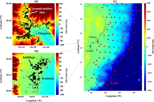
The 2011 disaster left an indelible mark on both areas. The experiences during the recovery process remain an insightful case study for understanding disaster mitigation. For this investigation, 1706 wooden houses in Onagawa and 6152 wooden houses in Iwanuma are examined to ascertain their vulnerability and to assess potential structural damage arising from multi-hazards. The wooden buildings in the considered exposure model are those surveyed during the post-2011 event tsunami building damage survey conducted by the Ministry of Land, Infrastructure, and Transportation of Japan (http://fukkou.csis.u-tokyo.ac.jp/dataset/list_all). Although the tsunami damage data include other building typologies, such as concrete, steel, and masonry structures, wooden buildings alone are focused upon in this study. This is because the multi-hazard loss estimation for non-wooden buildings was less reliable due to the lack of seismic fragility functions applicable to concrete, steel, or masonry types (Goda and De Risi 2018). Figure 1 illustrates the two locations of Onagawa and Iwanuma, along with their respective wooden buildings and hypothetical ground-motion sites (see the geographic locations where the PGV is evaluated using a ground-motion model in Figure 1(a)&(b)). Onagawa and Iwanuma are characterized by different coastal topographies; Onagawa is an area on Ria coast, whereas Iwanuma is an area on the coastal plain. Additionally, Figure 1(c) showcases the placement of 99 offshore sensors from the S-net.

Figure 1. Map of two coastal cities and monitoring sensors (figure modified from Li and Goda (2022)). (a) Zoomed map of Onagawa. (b) Zoomed map of Iwanuma. (c) Map of 99 offshore sensors from the S-net. The white points and the black triangles in (a) and (b) represent ground-motion sites (five in Onagawa and 10 in Iwanuma) and building assets, respectively.

3. Methods and data

3.1. Pre-processing of synthetic data

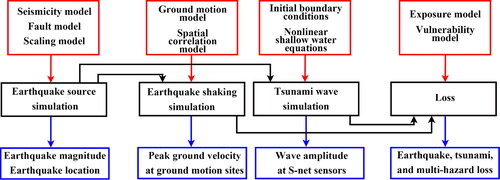
In this study, the data used for analysis and modelling are simulated, as illustrated in Figure 2. The simulated data encompass various aspects, including seismological data, shaking data, wave data, and loss data. Each type of data provides essential information related to the earthquake and tsunami events under investigation, enabling a comprehensive understanding of hazard characteristics and potential impacts. The following sections delve into the specific details of each type of the simulated data, shedding light on their generation and significance in the study. Since the methodologies for generating the synthetic data are fully detailed in Goda and De Risi (2018), the explanations are kept succinct.

Figure 2. Flowchart for simulating multi-hazard loss data. The loss refers to the cost of the damaged coastal buildings due to earthquake only, tsunami only, and multi-hazard (combined loss from both earthquake and tsunami).

3.1.1. Construction of stochastic earthquakes

In this study, a comprehensive analysis is conducted using a dataset consisting of 4000 stochastic earthquake source models, which has been used in the previous study (Li and Goda 2023). This study expands the data with seismic shaking data, earthquake loss data, multi-hazard loss data and includes an additional location, Onagawa. These earthquake source models cover a wide range of moment magnitudes (a measure of earthquake’s size), ranging from M7.5 to M9.1, with a discretization interval of 0.2 resulting in 500 models simulated per interval. This facilitates a thorough examination of various earthquake scenarios and their potential impacts. To generate these earthquake events, a Monte Carlo simulation approach is employed, following the methodology outlined by Goda et al. (2016). The methodology includes the simulation of the earthquake magnitude using a seismicity model that captures the distribution of earthquakes in the Tohoku region. This model is constructed based on earthquake catalogue data, which provide essential information on past seismic activity in the area. The earthquake epicentre and slip parameters are derived from a fault model and scaling model. The fault model represents the geometry and characteristics of the underlying fault responsible for generating the earthquakes. The scaling model relates the earthquake magnitude to the amount of slip on the fault and allows a synthesis of a heterogeneous slip distribution. This simulation technique enables the creation of many hypothetical earthquake scenarios, considering the inherent uncertainty associated with seismic events. Each earthquake event within the dataset is characterized by its specific magnitude and epicentre location (latitude and longitude). These parameters serve as the basic explanatory variables in the model development.

3.1.2. Ground shaking parameter simulation

To assess the seismic intensity for a specific earthquake source model, the study utilizes the PGV ground-motion model developed by Morikawa and Fujiwara (2013) to estimate the maximum absolute velocity of ground shaking caused by an earthquake. Additionally, to account for realistic distribution of the shaking effects, spatial correlation techniques are implemented to generate spatially correlated ground-motion data (Goda and De Risi 2018). In recognition of the greater number of building assets in Iwanuma (6152) compared to Onagawa (1706), this study strategically allocates a greater number of hypothetical ground-motion sites in Iwanuma. The PGV values are evaluated at 5 and 10 ground-motion sites located at Onagawa (Figure 1(a)) and Iwanuma (Figure 1(b)), respectively. This approach ensures that the estimation of seismic intensity and its associated impacts on the built environment are more accurately assessed, considering the specific characteristics of each location. By quantifying the seismic intensity by considering multiple ground-motion sites, the study aims to gain insights into the spatial distribution and severity of ground shaking in the targeted coastal areas. Figure 3(a)&(b) displays the PGV values in Onagawa and Iwanuma, respectively, for two specific scenarios (one having M8 and another having M9) whose heterogenous earthquake slip distributions are shown in Figure 4(a)&(c). Onagawa exhibits a higher sensitivity to PGV compared to Iwanuma, indicating that ground shaking is more pronounced in the former location. It can also be observed that larger magnitude earthquakes tend to result in higher PGV values, with a stronger and more intense ground-motion. On the other hand, Figure 3(c)&(d) shows the overall trends of the PGV values at the ground-motion sites in Onagawa and Iwanuma, respectively. The distributions of the average PGV reflect the local site conditions of the ground-motion sites in Onagawa and Iwanuma (e.g. site 1 in Onagawa and site 5 in Iwanuma are at stiff soil sites).

Figure 3. Peak ground velocity bar plot. (a) PGV recorded at the five ground-motion sites in Onagawa under two specific earthquakes (one having M8 and another having M9) that are shown in Figure 4(a)&(c). (b) PGV recorded at the 10 ground-motion sites in Iwanuma under two specific earthquakes (one having M8 and another having M9) that are shown in Figure 4(a)&(c). (c) Average PGV recorded at the five ground-motion sites in Onagawa based on 4000 earthquakes. (d) Average PGV recorded at the 10 ground-motion sites in Iwanuma based on 4000 earthquakes.

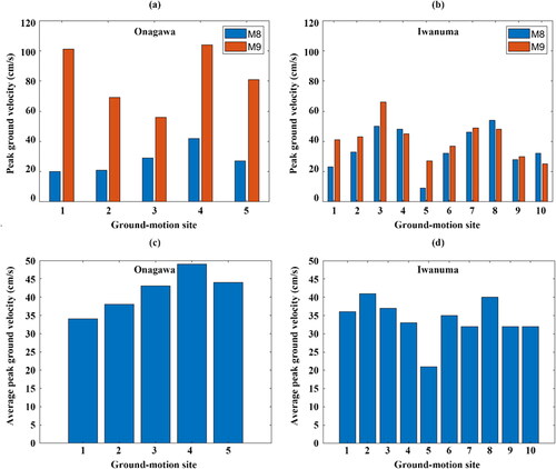
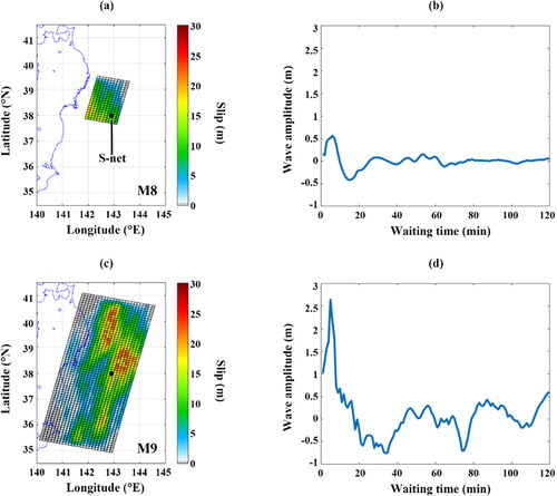
Figure 4. Earthquake rupture and wave time series plot. (a & b) The rupture of an earthquake and time series of the wave from one offshore sensor with a magnitude of 8. (c & d) The rupture of an earthquake and time series of the wave from one offshore sensor with a magnitude of 9. Higher magnitudes of earthquakes generally result in larger rupture sizes and higher wave amplitudes.

3.1.3. Tsunami wave amplitude and inland inundation

The simulation of tsunami waves begins immediately after the occurrence of an earthquake and continues for a duration of 120 min (Figure 4(b)&(d)). The estimation of the initial water surface elevation election is performed using formulas derived from Okada (1985) and Tanioka and Satake (1996). Then, the tsunami waves are simulated by solving nonlinear shallow water equations that describe the propagation and inundation of tsunamis, as outlined by Goto et al. (1997).

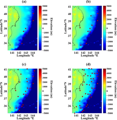
In this study, the maximum wave amplitude recorded by the S-net sensors within the first 5 min of the tsunami wave simulation is utilized as explanatory variables. These variables serve as input for the models developed to predict tsunami loss, which is the response variable of interest. Based on the previous study of Li and Goda (2022), two key findings are highlighted. Firstly, the maximum wave amplitudes recorded by offshore sensors during this initial 5-min period contains valuable information for tsunami loss analysis. Secondly, given the number of selected offshore sensors (5, 10, 20, or 40), according to the Akaike Information Criterion (AIC), different selection strategies are applied for placement of their optimal locations (Figure 5). When the number of sensors available is small, placing farther from the coastline is preferable, since it can detect the high wave amplitude earlier. When a larger number of sensors are available, the selected offshore sensors tend to spread from offshore to nearshore, since they can achieve both early detection and improved estimation of the potential impact to the coastal areas.

Figure 5. Maps of selected offshore sensors with varies densities. (a) Locations of the first five offshore sensors selected by AIC. (b) Locations of the first 10 offshore sensors selected by AIC. (c) Locations of the first 20 offshore sensors selected by AIC. (d) Locations of the first 40 offshore sensors selected by AIC. Those will be used in the results section for comparison.

3.1.4. Estimation of direct shaking and tsunami loss from vulnerability assessments

The response variable in this study is the loss, which consists of earthquake loss, tsunami loss, and multi-hazard loss. The loss estimation is performed for individual buildings using Monte Carlo simulations. More details can be found in Goda and De Risi (2018).

The earthquake loss in Onagawa (Figure 6(a)) and Iwanuma (Figure 7(a)) is calculated by applying appropriate exposure (6152 wooden houses in Iwanuma valued US$ 1280 million and 1706 wooden houses in Onagawa valued US$ 355 million) and seismic fragility models for Japanese wooden buildings (Yamaguchi and Yamazaki 2001; Midorikawa et al. 2011; Wu et al. 2016) to ground shaking intensities (Section 3.1.2). For the seismic fragility functions, three models are weighted equally (Goda and De Risi 2018). The damage states for shaking are defined as: partial damage, half collapse, and complete collapse, and the corresponding damage ratios are assigned as 0.03–0.2, 0.2–0.5, and 0.5–1.0, respectively (Kusaka et al. 2015). The tsunami loss in Onagawa (Figure 6(b)) and Iwanuma (Figure 7(b)) is computed by employing suitable exposure and tsunami fragility models (De Risi et al. 2017) in conjunction with precalculated tsunami inundation data (Section 3.1.3). For tsunami damage, the following five damage states are considered: minor, moderate, extensive, complete, and collapse, together with the damage ratios of 0.03–0.1, 0.1–0.3, 0.3–0.5, 0.5–1.0, and 1.0, respectively, according to the Ministry of Land, Infrastructure, and Transportation of Japan’s tsunami damage assessment guideline.

Figure 6. Loss data for Onagawa, modified from Li and Goda (2022). (a) Earthquake loss. (b) Tsunami loss. (c) Multi-hazard loss.

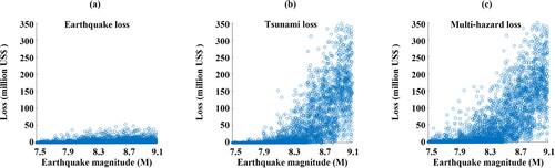
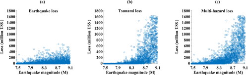
Figure 7. Loss data for Iwanuma, modified from Li and Goda (2022). (a) Earthquake loss. (b) Tsunami loss. (c) Multi-hazard loss.

Subsequently, for each building, the final damage ratio is determined by taking the maximum of the estimated shaking and tsunami damage ratios (Goda and De Risi 2018). This simplistic approach for computing the multi-hazard loss does not account for damage accumulation from sequential ground-motion and tsunami hazards. Finally, the multi-hazard loss value (e.g. Figure 6(c) for Onagawa and Figure 7(c) for Iwanuma) is calculated by sampling a value of the building replacement cost from the lognormal distribution and multiplying it by the final damage ratio. The building replacement cost for wooden buildings is estimated based on the regional unit-area construction cost statistics (mean = 1600 USD/m² and coefficient of variation = 0.33) from a construction costing handbook and the regional floor area statistics collected by the Ministry of Land, Infrastructure, and Transportation of Japan (mean = 130 m² and coefficient of variation = 0.33).

Due to the higher number of building assets, Iwanuma is more susceptible to large loss compared to Onagawa. Iwanuma, being on a coastal plain and wide open, is more exposed to tsunami waves, resulting in substantial damage when the earthquake magnitude is relatively large, exceeding M8.5. While Onagawa is more prone to experiencing severe loss when the earthquake magnitude surpasses M8.3, as it is situated in a Ria coastal location that intensifies the coastal inundation during a tsunami event. To encompass the overall multi-hazard loss within a broader region, this study combines the individual earthquake, tsunami, and multi-hazard losses from Onagawa and Iwanuma to calculate the joint loss (Figure 8). This approach allows for a comprehensive assessment of the combined impact of these hazards, providing valuable insights into the regional risk management.

Figure 8. Joint loss data of Onagawa and Iwanuma. (a) Earthquake loss. (b) Tsunami loss. (c) Multi-hazard loss.

3.2. Model fitting and performance metrics

3.2.1. Random forest

In this study, a RF model is trained by randomly selecting a subset of nodes from the earthquake information, ground-motion sites, and offshore sensors for each decision tree. The algorithm calculates the mean square error (MSE) for each possible split of the features, evaluating their performance in reducing the error. The algorithm then identifies the feature that achieves the lowest MSE as the best split for the data. The decision tree construction process continues until the MSE cannot be further improved or the maximum number of allowed splits is reached. It is important to note that each decision tree is built using bootstrap sampling, where some tsunami events may be selected repeatedly while others may not be included at all (Breiman 1996; Nordhausen 2009).

The training algorithm for bootstrap in RF can be summarized as follows. Starting with a training dataset that includes explanatory variables $X=x_1,\dots ,x_n$ and the corresponding response variable $Y=y_1,\dots ,y_n,\mathrm{ }$ the bagging process is repeated $B$ times to fit decision trees. Each time, a random subset of the training data is selected for training a decision tree. By using the bootstrap method, bagging helps reduce overfitting and improves the accuracy and stability of the model. The key idea is that each decision tree within the RF is trained using a slightly different subset of the training data, resulting in a diverse ensemble of trees. This diversity allows the RF to capture a wide range of patterns and make robust predictions. Once all decision trees are trained, the final prediction is obtained by averaging the results from each individual tree, as shown in Eq. (1)(1) $$\widehat{f}=\mathrm{ }\frac{1}{B}\sum _{b=1}^B{f}_b\left(x\right)$$(1) : (1) $$\widehat{f}=\mathrm{ }\frac{1}{B}\sum _{b=1}^B{f}_b\left(x\right)$$(1) This ensemble approach combines the knowledge of multiple trees and reduces the impact of individual outliers or noisy data points, resulting in a more reliable and accurate prediction (Figure 9).

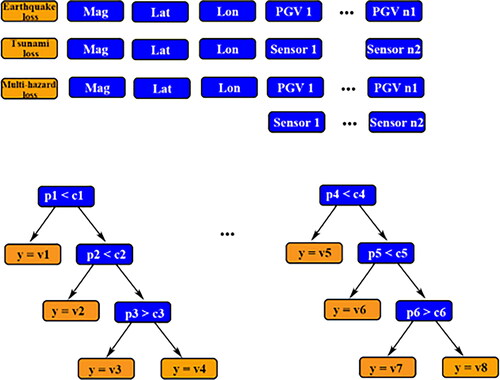
Figure 9. Random forest process. The orange and blue grids represent the response and explanatory variables, respectively. The response variables include earthquake, tsunami, and multi-hazard loss and explanatory variables include earthquake magnitude, epicentre location, PGV, and wave amplitude from offshore sensors. ‘p’ represents parameter selected from the explanatory variables and ‘c’ represents a criterion. ‘y’ represents the response variables and ‘v’ represents a value assigned to ‘y’.

A systematic preliminary investigation is conducted by adjusting the maximum depth parameter of the decision tree. The decision tree in the RF model is constrained to a maximum of 10 splits to strike a balance between computational efficiency and predictive accuracy. The RF model comprises 500 decision trees, chosen to ensure a reliable estimation of tsunami loss without incurring excessive computational burden. To obtain the final prediction of multi-hazard loss, the RF model takes the mean of the predictions made by all the decision trees in the forest. This ensemble approach leverages the collective knowledge and diversity of the individual trees, resulting in a robust and reliable estimation of the multi-hazard loss.

3.2.2. Model performance comparison metrics

The MSE is a commonly used metric to evaluate the goodness of fit of a model to the data. It quantifies the average of the sum of squared errors. The MSE can be expressed as: (2) $$\mathrm{MSE}=\mathrm{ }\frac{1}{n}\sum _1^n(y_i-{\widehat{y}}_i{)}^2$$(2)

The MSE provides a measure of how well the model predicts the observed data, with a lower MSE indicating a better fit.

An alternative metric is the R-squared ($R^2$) value of the original data and the predicted data, which is also known as the coefficient of determination and measures the proportion of the variance in the response variable that can be explained by the explanatory variables in a regression model. The $R^2$ can be expressed as: (3) $$R^2\mathrm{ }=\mathrm{ }1\text{-}\mathrm{ }\frac{\sum _1^n(y_i-{\widehat{y}}_i{)}^2}{\sum _1^n(y_i-{\overline{y}}_i{)}^2}$$(3)

A higher $R^2$ value explains a larger proportion of the variability in the response variable which provides a better fit to the data.

4. Results

In this section, the performances of the RF models in estimating three types of losses are evaluated. To examine the effectiveness of monitoring sensor networks, different densities (numbers) of ground-motion sites and offshore sensors are compared. The study considers four levels of ground-motion sites: none (0 used), small (20% used), medium (60% used), and large (100% used). The large (or 100% used) cases consider 10 and 5 ground-motion sites in Iwanuma and Onagawa, respectively (Figure 1(a)&(b)). In the small density scenario for the ground-motion sites, two ground-motion sites are used in Iwanuma and one in Onagawa. The selection of ground-motion sites is based on a random uniform sampling approach, with a focus on locations where buildings are concentrated. This comparison allows for an assessment of how efficiently monitoring sensors can contribute to the accuracy of earthquake loss estimation.

For the offshore sensors, this study considers five levels: 0 sensors, 5 sensors, 10 sensors, 20 sensors, and 40 sensors. In the previous study by Li and Goda (2022), an order of offshore sensors based on the AIC score was determined (Figure 5). This order provides a ranking of the sensors that contribute the most to improving accuracy, considering spatial and temporal characteristics of the waves and the sensor positions. It has been observed that at the beginning of an earthquake, farther offshore sensors provide useful information, while as time progresses, sensors closer to the coastline become more informative. In this study, the previously determined order is used to select the corresponding number of sensors for each of the five levels mentioned above. The following sections provide in-depth analyses of earthquake, tsunami, and multi-hazard loss. Each section focuses on the specific details and characteristics of these hazards, exploring various factors that contribute to their impact and evaluating the associated losses.

4.1. Earthquake only loss estimation

The first type of loss estimated in this study is the earthquake loss. The earthquake loss serves as the response variable, and the explanatory variables include earthquake information (magnitude and epicentre location), and PGV at different ground-motion sites. Table 1 provides an overview of the MSE and $R^2\mathit{ }$ values for four different models under the joint loss as well as the individual loss estimations for Iwanuma and Onagawa. The primary focus of this study is the estimation of joint loss, while the loss estimations for the two separate locations are considered. The results clearly indicate that as the number of ground-motion sites increases, the MSE values decrease. When a small number of ground-motion sites (one in Onagawa and two in Iwanuma) are used, it results in a 60% reduction of the MSE compared to the base model, where no ground-motion sites are used (also can be seen from Figure 10(a)&(b)). When a larger number of ground-motion sites (five in Onagawa and 10 in Iwanuma) are utilized, there is an 80% reduction in the MSE (also can be seen from Figure 10(a)&(c)). The RF algorithm alone cannot improve the estimation if the data lacks significant information regarding the loss, such as the cases with seismological data alone. Therefore, it is crucial to have both high-quality data and a well-performing algorithm to achieve accurate loss estimation. Similarly, the $R^2$ values obtained for the different models further support the observations made regarding the MSE values. Higher $R^2$ values indicate a better fit and performance of the models in explaining the variation in earthquake loss. As the density of ground-motion sites increases, the $R^2$ values tend to increase, indicating an improved ability of the models to capture and explain the earthquake loss variation accurately.

Figure 10. Plots of simulated joint (two locations) earthquake loss with predicted loss. Panels (a)–(c) correspond to none, small, and large density of ground-motion sites, respectively. The importance of ground-motion sites is compared.

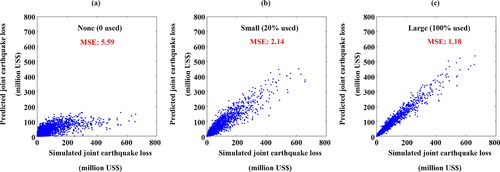
Table 1. MSE and $R^2\mathit{ }$ for earthquake loss estimation under randomly selected different numbers of ground-motion sites.

Number of ground-motion sites	Joint		Iwanuma		Onagawa
	MSE	$R^2$	MSE	$R^2$	MSE	$R^2$
None (0 used)	5.694	74.39%	8.203	67.56%	8.929	63.06%
Small (20% used)	2.140	90.38%	2.990	88.15%	3.127	87.08%
Medium (60% used)	1.404	93.69%	2.079	91.79%	1.797	92.56%
Large (100% used)	1.176	94.69%	1.772	92.94%	1.340	94.46%

Small (1 & 2); medium (3 & 6); large (5 & 10) for Onagawa and Iwanuma, respectively.

These suggest that incorporating ground-motion sites leads to accurate earthquake loss estimation, as it captures a broader spatial representation of the seismic intensity. Besides, these reinforce the importance of incorporating a higher density of ground-motion sites in earthquake loss estimation, as it leads to more reliable and informative models for assessing and understanding the impact of earthquakes on the loss.

4.2. Tsunami only loss estimation

The second focus of this study is the estimation of tsunami loss. In this case, the response variable is the tsunami loss, and the explanatory variables consist of earthquake information (magnitude and epicentre location) and wave amplitudes at various offshore sensors. Table 2 presents the MSE and $R^2$ values for five different models. These metrics offer insights into the accuracy and performance of the models in estimating tsunami loss. When incorporating five offshore sensors in the model, there is a 25% decrease in the MSE compared to the base model (also can be seen from Figure 11(a)&(b)), where no offshore sensors are utilized. This indicates that the inclusion of offshore sensor data contributes to improving the accuracy of tsunami loss estimation. Furthermore, by increasing the number of offshore sensors to 40, the MSE is further reduced by 45% (also can be seen from Figure 11(a)&(c)), highlighting the significant impact of additional sensor information on enhancing the accuracy of the estimation.

Figure 11. Plots of simulated joint (two locations) tsunami loss with predicted loss. Panels (a)–(c) correspond to 0 sensor, 5 sensors, and 40 sensors, respectively. The importance of offshore sensors is compared.

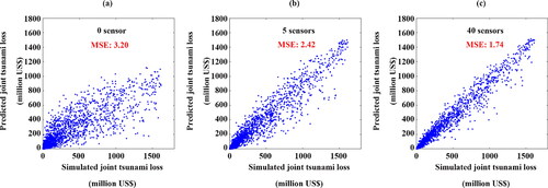
Table 2. MSE and $R^2$ for tsunami loss estimation under different densities of offshore sensors.

Density of offshore sensors	Joint		Iwanuma		Onagawa
	MSE	$R^2$	MSE	$R^2$	MSE	$R^2$
0 sensor	3.198	90.08%	3.359	89.07%	4.610	86.89%
5 sensors	2.423	92.44%	2.344	92.38%	3.703	89.46%
10 sensors	2.084	93.55%	2.027	93.42%	3.134	91.09%
20 sensors	1.958	93.94%	1.959	93.64%	2.875	91.84%
40 sensors	1.736	94.62%	1.747	94.31%	2.628	92.53%

4.3. Multi-hazard loss estimation

The primary objective and novelty of this study are to estimate multi-hazard loss, which includes both earthquake and tsunami impacts. The multi-hazard loss serves as the response variable, and a combination of explanatory variables is utilized. These variables include earthquake information (magnitude and epicentre location), PGV obtained from different ground-motion sites, and wave amplitude data collected from various offshore sensors. In the multi-hazard loss estimation, both seismic and tsunami monitoring sensors are considered.

Figure 12 shows the MSE as a function of portion of ground-motion sites and the number of offshore sensors. Notably, in terms of the number of ground-motion sites (Figure 12(b)), there is a substantial difference between the scenario with no ground-motion sites and the one with a small portion of ground-motion sites. As the number of ground-motion sites increases, the MSE reduction becomes more gradual and less substantial, like the trend of offshore sensors. Figure 12(c) reveals a noticeable trend of decreasing MSE as the number of offshore sensors increases. The initial addition of the first five sensors results in a substantial reduction in MSE, indicating a significant improvement in the model’s performance. As more sensors are added beyond this point, the decrease in MSE becomes less pronounced. Table 3 summarizes the MSE and $R^2$ values for the multi-hazard models. Figure 13 shows scatter plots of simulated joint multi-hazard loss with predicted loss for visual inspection of the similarity of the simulated and predicted data. The results demonstrate the impact of incorporating different combinations of monitoring sensors on the performance of the multi-hazard loss estimation. When considering only offshore sensors in the joint multi-hazard estimation model, there is on average a 10% decrease in the MSE compared to the base model, which does not utilize any offshore sensors or ground-motion sites. When incorporating only ground-motion sites in the multi-hazard estimation model, there is on average a 40% decrease in the MSE compared to the base model.

Figure 12. 3-D MSE of the joint (two locations) multi-hazard loss plot in terms of density of offshore sensors and ground-motion sires. (a) 3D plot (N, S, M, L represent none, small, medium, large portions of ground-motion sites, respectively). (b) MSE of joint multi-hazard loss vs. portion of ground-motion sites. (c) MSE of joint multi-hazard loss vs. number of offshore sensors.

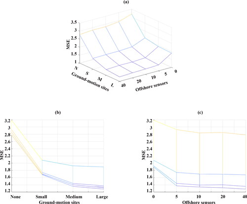
Figure 13. Plots of simulated joint (two locations) multi-hazard loss with predicted loss. Panels (a)–(c) correspond to 0 sensor & no ground-motion sites, five sensors & small ground-motion sites, and 40 sensors & large ground-motion sites, respectively. The importance of joint monitoring sensors is compared.

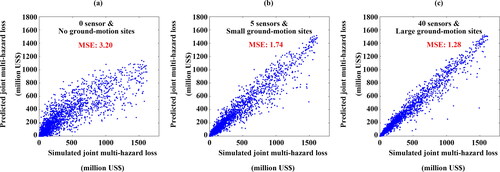
Table 3. MSE and $R^2$ for joint multi-hazard loss under different densities of ground-motion sites and offshore sensors: small (1 & 2), medium (3 & 6), large (5 & 10) for Onagawa and Iwanuma, respectively.

Density of ground-motion sites	Density of offshore sensors	MSE	$R^2$
None (0 used)	0 sensor	3.188	86.08%
	5 sensors	2.928	87.20%
	10 sensors	2.835	87.56%
	20 sensors	2.846	87.94%
	40 sensors	2.781	87.79%
Small (20% used)	0 sensor	2.081	90.92%
	5 sensors	1.744	92.37%
	10 sensors	1.700	92.56%
	20 sensors	1.695	93.80%
	40 sensors	1.678	94.09%
Medium (60% used)	0 sensor	1.927	91.56%
	5 sensors	1.442	93.68%
	10 sensors	1.396	93.87%
	20 sensors	1.404	93.80%
	40 sensors	1.359	94.09%
Large (100% used)	0 sensor	1.896	91.69%
	5 sensors	1.374	93.49%
	10 sensors	1.341	94.10%
	20 sensors	1.321	94.15%
	40 sensors	1.284	94.40%

Furthermore, when utilizing a sparse density of joint monitoring sensors (consisting of a small number of ground-motion sites and five offshore sensors) in the multi-hazard estimation model, there is a significant 45% decrease in the MSE compared to the base model. This performance surpasses all scenarios using only offshore sensors or only ground-motion sites. As the density of joint monitoring sensors increases (with a large portion of ground-motion sites and 40 offshore sensors), there is an impressive 60% decrease in the MSE compared to the base model. These results (see Table 3) highlight the effectiveness of joint monitoring sensors in capturing the characteristics of multi-hazard loss resulting from both earthquakes and tsunamis.

5. Discussion

It is important to recognize the limitations of this study. A notable limitation is the use of hypothetical datasets for earthquake and tsunami events. Due to the scarcity of significant historical tsunami events, even in regions with extensive offshore monitoring systems, real-world data are limited. To overcome this challenge, synthetic data were employed to simulate a wide range of earthquake and tsunami scenarios. While this allowed for comprehensive analysis, it is crucial to recognize that synthetic data may not fully capture the complexity and variability of real-world events. In other words, the results shown in Section 4 entail model errors (i.e. differences between the real situations and model predictions). The sources of the model errors can be attributed to the components of the multi-hazard catastrophe model, including earthquake sources, ground-motion intensity simulations, tsunami wave simulations, single-hazard and multi-hazard loss generations (affected by the adopted seismic fragility functions, tsunami fragility functions, building replacement cost models, and ignorance of the shaking-tsunami damage accumulation effects; see Section 2). These could introduce potential biases in the results and limit the generalization of the findings.

This article promotes the accessibility of the data and algorithms (see Code Availability) used in the study, enabling interested researchers and practitioners to replicate and further advance the multi-hazard loss estimation methods. Future research should aim to incorporate more real-world data to further validate and refine the proposed models, considering additional variables and exploring their applicability in diverse geographic regions and hazard scenarios.

6. Conclusions

This study introduced a novel approach to estimate multi-hazard loss resulting from earthquakes and tsunamis using machine learning techniques. The RF algorithm was employed, leveraging hypothetical simulated data at seismic and tsunami monitoring sensors, including ground-motion sites and offshore sensors. This study revealed that increasing the density of ground-motion sites and offshore sensors significantly improved the model’s performance. The inclusion of monitoring sensors, both seismic and tsunami, provided valuable information for capturing the complex dynamics and interplay between various variables influencing the losses. Notably, the study highlighted the importance of joint monitoring sensors in estimating multi-hazard loss. By integrating both ground-motion sites and offshore sensors in the multi-hazard estimation model, a significant improvement was achieved compared to scenarios using only one type of sensors. This demonstrated the robustness and accuracy of the joint monitoring approach in accounting for the combined effects of earthquakes and tsunamis.

The findings of this study have significant implications for disaster risk management and community recovery efforts. Accurate estimation of multi-hazard losses can greatly enhance decision-making processes and resource allocation. By leveraging machine learning techniques and comprehensive monitored data, policymakers and stakeholders can gain deeper insights into the risks associated with earthquakes and tsunamis, leading to more effective mitigation strategies and improved resilience of coastal communities.

Disclosure statement

The authors declare that they have no known competing financial interests or personal relationships that could have appeared to influence the work reported in this article.

Code availability

The source codes are available for downloading at the link: https://github.com/YaoLi074/Multi-hazard.git and https://github.com/YaoLi074/TEW-RF.git.

Additional information

Funding

The work is funded by the Canada Research Chair Program [950-232015] and the NSERC Discovery Grant [RGPIN-2019-05898].

References

- Benchekroun S, Omira R, Baptista MA, Mouraouah AE, Brahim AI, Toto EA. 2015. Tsunami impact and vulnerability in the harbour area of Tangier, Morocco. Geomatics Nat Hazards Risk. 6(8):718–740. doi: 10.1080/19475705.2013.858373.
- Breiman L. 1996. Bagging predictors. Mach Learn. 24(2):123–140. doi: 10.1007/BF00058655.
- Breiman L. 2001. Random forest. Mach Learn. 45(1):5–32. doi: 10.1023/A:1010933404324.
- Crowell BW, Melgar D, Geng J. 2018. Hypothetical real‐time GNSS modeling of the 2016 Mw 7.8 Kaikōura earthquake: perspectives from ground motion and tsunami inundation prediction. Bull Seismol Soc Am. 108(3B):1736–1745. doi: 10.1785/0120170247.
- De Risi R, Goda K, Yasuda T, Mori N. 2017. Is flow velocity important in tsunami empirical fragility modeling? Earth Sci Rev. 166:64–82. doi: 10.1016/j.earscirev.2016.12.015.
- Duwal S, Liu D, Pradhan PM. 2023. Flood susceptibility modeling of the Karnali river basin of Nepal using different machine learning approaches. Geomat Nat Hazards Risk. 14(1). doi: 10.1080/19475705.2023.2217321.
- Elkady A, Güell G, Lignos DG. 2020. Proposed methodology for building‐specific earthquake loss assessment including column residual axial shortening. Earthq Eng Struct Dyn. 49(4):339–355. doi: 10.1002/eqe.3242.
- Erdik M, Şeşetyan K, Demircioğlu MB, Hancılar U, Zülfikar C. 2011. Rapid earthquake loss assessment after damaging earthquakes. Soil Dyn Earthq Eng. 31(2):247–266. doi: 10.1016/j.soildyn.2010.03.009.
- Ghimire S, Guéguen P, Giffard-Roisin S, Schorlemmer D. 2022. Testing machine learning models for seismic damage prediction at a regional scale using building-damage dataset compiled after the 2015 Gorkha Nepal earthquake. Earthq Spectra. 38(4):2970–2993. doi: 10.1177/87552930221106495.
- Goda K. 2021. Multi-hazard parametric catastrophe bond trigger design for subduction earthquakes and tsunamis. Earthq Spectra. 37(3):1827–1848. doi: 10.1177/8755293020981974.
- Goda K, De Risi R. 2018. Multi-hazard loss estimation for shaking and tsunami using stochastic rupture sources. Int J Disaster Risk Reduct. 28:539–554. doi: 10.1016/j.ijdrr.2018.01.002.
- Goda K, Mori N, Yasuda T. 2019. Rapid tsunami loss estimation using regional inundation hazard metrics derived from stochastic tsunami simulation. Int J Disaster Risk Reduct. 40:101152. doi: 10.1016/j.ijdrr.2019.101152.
- Goda K, Yasuda T, Mori N, Maruyama T. 2016. New scaling relationships of earthquake source parameters for stochastic tsunami simulation. Coast Eng J. 58(3):1650010–1–1650010-40. doi: 10.1142/S0578563416500108.
- Gomez Zapata JC, Pittore M, Brinckmann N, Lizarazo-Marriaga J, Medina S, Tarque N, Cotton F. 2023. Scenario-based multi-risk assessment from existing single-hazard vulnerability models. An application to consecutive earthquakes and tsunamis in Lima, Peru. Nat Hazards Earth Syst Sci. 23(6):2203–2228. doi: 10.5194/nhess-23-2203-2023.
- Goto C, Ogawa Y, Shuto N.1997. Imamura, F. Numerical method of tsunami simulation with the leap-frog scheme. IOC Manual 35. Paris, France: UNESCO.
- Ho TK. 1998. The random subspace method for constructing decision forests. IEEE Trans Pattern Anal Mach Intell. 20(8):832–844. doi: 10.1109/34.709601.
- Jaffe BE, Borrero JC, Prasetya G, Peters RFY, McAdoo BG, Gelfenbaum G, Morton RA, Ruggiero P, Higman B, Dengler L, et al. 2006. Northwest Sumatra and Offshore Islands Field Survey after the December 2004 Indian Ocean Tsunami. Earthq Spectra. 22(3_suppl):105–135. doi: 10.1193/1.2207724.
- Jaiswal K, Wald DJ, Earle PS, Porter K, Hearne M. 2010. Earthquake casualty models within the USGS prompt assessment of global earthquakes for response (PAGER) system. In: Advances in Natural and Technological Hazards Research. Netherlands: Springer Nature. p. 83–94. doi: 10.1007/978-90-481-9455-1_6.
- Karakas G, Kocaman S, Gokceoglu C. 2023. A hybrid multi-hazard susceptibility assessment model for a basin in Elazig Province, Türkiye. Int J Disaster Risk Sci. 14(2):326–341. doi: 10.1007/s13753-023-00477-y.
- Kusaka A, Ishida H, Torisawa K, Doi H, Yamada K. 2015. Vulnerability functions in terms of ground motion characteristics for wooden houses evaluated by use of earthquake insurance experience. AIJ J Techn Des. 21(48):527–532. doi: 10.3130/aijt.21.527.
- Li Y, Goda K. 2022. Hazard and risk-based tsunami early warning algorithms for ocean bottom sensor S-net system in Tohoku, Japan, using sequential multiple linear regression. Geosciences. 12(9):350. doi: 10.3390/geosciences12090350.
- Li Y, Goda K. 2023. Risk-based tsunami early warning using random forest. Comput Geosci. 179:105423. doi: 10.1016/j.cageo.2023.105423.
- Liu Y, Zhang X, Liu W, Lin Y, Su F, Cui J, Wei B, Cheng H, Gross L. 2023. Seismic vulnerability and risk assessment at the urban scale using support vector machine and GIScience technology: a case study of the Lixia District in Jinan City, China. Geomat Nat Hazards Risk. 14(1). doi: 10.1080/19475705.2023.2173663.
- Midorikawa S, Ito Y, Miura H. 2011. Vulnerability functions of buildings based on damage survey data of earthquakes after the 1995 Kobe earthquake. J Jpn Assoc Earthq Eng. 11(4):4_34–4_47. doi: 10.5610/jaee.11.4_34.
- Mohajane M, Costache R, Karimi F, Pham QB, Essahlaoui A, Nguyen H, Laneve G, Oudija F. 2021. Application of remote sensing and machine learning algorithms for forest fire mapping in a Mediterranean area. Ecol Indic. 129:107869. doi: 10.1016/j.ecolind.2021.107869.
- Mori N, Takahashi T, THE 2011 TOHOKU EARTHQUAKE TSUNAMI JOINT SURVEY GROUP. 2012. Nationwide post event survey and analysis of the 2011 Tohoku earthquake tsunami. Coast Eng J. 54(1):1250001–1–1250001-27. doi: 10.1142/S0578563412500015.
- Morikawa N Fujiwara H. 2013. A new ground motion prediction equation for Japan applicable up to M9 mega-earthquake. J Disaster Res. 8(5):878–888.
- Negulescu C, Benaichouche A, Lemoine A, Roy SL, Pedreros R. 2020. Adjustability of exposed elements by updating their capacity for resistance after a damaging event: application to an earthquake–tsunami cascade scenario. Nat Hazards. 104(1):753–793. doi: 10.1007/s11069-020-04189-0.
- Nordhausen K. 2009. The elements of statistical learning: data mining, inference, and prediction, second edition by Trevor Hastie, Robert Tibshirani, Jerome Friedman. Int Stat Rev. 77(3):482–482. doi: 10.1111/j.1751-5823.2009.00095_18.x.
- Okada Y. 1985. Surface deformation due to shear and tensile faults in a half-space. Bull Seismol Soc Am. 75(4):1135–1154. doi: 10.1785/BSSA0750041135.
- Okada Y, Kasahara K, Hori S, Obara K, Sekiguchi S, Fujiwara H, Yamamoto A. 2004. Recent progress of seismic observation networks in Japan—Hi-net, F-net, K-NET and KiK-net—. Earth Planet Sp. 56(8):xv–xxviii. doi: 10.1186/BF03353076.
- Park H, Alam MS, Cox DT, Barbosa AR, van de Lindt JW. 2019. Probabilistic seismic and tsunami damage analysis (PSTDA) of the Cascadia Subduction Zone applied to Seaside, Oregon. Int J Disaster Risk Reduct. 35:101076. doi: 10.1016/j.ijdrr.2019.101076.
- Park S, Lee D. 2020. Prediction of coastal flooding risk under climate change impacts in South Korea using machine learning algorithms. Environ Res Lett. 15(9):094052. doi: 10.1088/1748-9326/aba5b3.
- Piao Y, Lee D, Park S, Kim HG, Jin Y. 2022. Multi-hazard mapping of droughts and forest fires using a multi-layer hazards approach with machine learning algorithms. Geomat Nat Hazards Risk. 13(1):2649–2673. doi: 10.1080/19475705.2022.2128440.
- Raduszynski T, Numada M. 2023. Measure and spatial identification of social vulnerability, exposure and risk to natural hazards in Japan using open data. Sci Rep. 13(1):664. doi: 10.1038/s41598-023-27831-w.
- Ranjbar HR, Dehghani H, Ardalan A, Saradjian MR. 2017. A GIS-based approach for earthquake loss estimation based on the immediate extraction of damaged buildings. Geomat Nat Hazards Risk. 8(2):772–791. doi: 10.1080/19475705.2016.1265013.
- Sanderson DR, Cox DT. 2023. Comparison of national and local building inventories for damage and loss modeling of seismic and tsunami hazards: from parcel- to city-scale. Int J Disaster Risk Reduct. 93:103755. doi: 10.1016/j.ijdrr.2023.103755.
- Scheingraber C, Käser M. 2020. Spatial seismic hazard variation and adaptive sampling of portfolio location uncertainty in probabilistic seismic risk analysis. Nat Hazards Earth Syst Sci. 20(7):1903–1918. doi: 10.5194/nhess-20-1903-2020.
- Shirzadi A, Shahabi H, Chapi K, Bui DT, Pham BT, Shahedi K, Ahmad BB. 2017. A comparative study between popular statistical and machine learning methods for simulating volume of landslides. Catena. 157:213–226. doi: 10.1016/j.catena.2017.05.016.
- Tanioka Y, Satake K. 1996. Tsunami generation by horizontal displacement of ocean bottom. Geophys Res Lett. 23(8):861–864. doi: 10.1029/96GL00736.
- Tehrani FS, Santinelli G, Herrera MH. 2021. Multi-regional landslide detection using combined unsupervised and supervised machine learning. Geomat Nat Hazards Risk. 12(1):1015–1038. doi: 10.1080/19475705.2021.1912196.
- Uehira K, Kanazawa T, Mochizuki M, Fujimoto H, Noguchi S, Shinbo T, Shiomi K, Kunugi T, Aoi S, Matsumoto T, et al. 2016. Outline of seafloor observation network for earthquakes and tsunamis along the Japan Trench (S-net). EGU General Assembly Conference Abstracts. http://ui.adsabs.harvard.edu/abs/2016EGUGA.1813832U/abstract.
- Virtriana R, Harto AB, Atmaja FW, Meilano I, Fauzan KN, Anggraini TS, Ihsan KTN, Mustika FA, Suminar W. 2023. Machine learning remote sensing using the random forest classifier to detect the building damage caused by the Anak Krakatau Volcano tsunami. Geomat Nat Hazards Risk. 14(1):28–51. doi: 10.1080/19475705.2022.2147455.
- Wu H, Masaki K, Irikura K, Kurahashi S, Disaster Prevention Research Center, Aichi Institute of Technology Yachigusa 1247, Yakusa-cho, Toyota, Japan. 2016. Empirical fragility curves of buildings in Northern Miyagi prefecture during the 2011 off the Pacific Coast of Tohoku earthquake. J Disaster Res. 11(6):1253–1270. doi: 10.20965/jdr.2016.p1253.
- Xia J, Li Y, Cheng Y, Li J, Tian S. 2021. Research on compressive sensing of strong earthquake signals for earthquake early warning. Geomat Nat Hazards Risk. 12(1):694–715. doi: 10.1080/19475705.2021.1889689.
- Yalcin I, Kocaman S, Gokceoglu C. 2020. A CitSci approach for rapid earthquake intensity mapping: a case study from Istanbul (Turkey). IJGI. 9(4):266. doi: 10.3390/ijgi9040266.
- Yamaguchi N, Yamazaki F. 2001. Estimation of strong motion distribution in the 1995 Kobe earthquake based on building damage data. Earthq Eng Struct Dyn. 30(6):787–801. doi: 10.1002/eqe.33.
- Zhang R, Duan K, You S, Wang F, Tan SM. 2020. A novel remote sensing detection method for buildings damaged by earthquake based on multiscale adaptive multiple feature fusion. Geomat Nat Hazards Risk. 11(1):1912–1938. doi: 10.1080/19475705.2020.1818637.