Geological and hydrogeological drivers of seismic deformation in L’Aquila, Italy: insights from InSAR analysis

Abstract

Historical and recent earthquakes have struck the city of L'Aquila, located in the axial zone of the Central Apennines, Italy, causing severe damage to the historic centre. Recent studies have shown that higher intensity of damage to buildings in L’Aquila downtown, both in the case of the 2009 earthquake (Mw: 6.29) and the 1703 earthquake (Mw: 6.7), is associated with higher post-seismic subsidence rates, detected through A-DInSAR maps, in the time range 2010–2021. This finding suggests the existence of geological factors that drive deformation (and building damage). The availability of long time series of InSAR data acquired from the Cosmo-SkyMed and Sentinel-1 missions, has enabled us to analyze the relationships between ground deformations and geological, hydrogeological, and geomorphological factors that may affect them. The correlation analysis between predisposing factors and SAR deformation has highlighted an increase in subsidence strongly conditioned by the outcropping lithology, showing how compositional variations within lithology can significantly influence ground deformations. Furthermore, hydrogeology has been recognized as playing an important role in determining deformation processes: the water table depth locally influences long-term subsidence, while seasonal fluctuations in the water table may be responsible for secondary areal variations in ground deformations.

Keywords:

• A-DInSAR
• high-risk seismic areas
• L’Aquila earthquake
• seismic damage
• correlation analysis

1. Introduction

The study of pre- and post-seismic ground behavior is of increasing importance in the framework of seismic risk mitigation and predicting the local seismic effects induced by earthquake is of course crucial for urban planning. For this reason, the use of Advanced Synthetic Aperture Radar Interferometry (A-DInSAR) (Ferretti et al. 2001; Berardino et al. 2002) has become increasingly common, especially in urban contexts (Lanari et al. 2010; Martino et al. 2022). This technology offers advantages such as relatively low costs, the ability to cover extensive areas, millimetric accuracy, and the capability to investigate long temporal time ranges (Cigna et al. 2011; Tomás et al. 2014; Ezquerro et al. 2020; Nappo et al. 2020; Wang et al. 2024).

Therefore, in this presented case-study, the comparison of A-DInSAR data of L’Aquila historic center, hit by the April 6, 2009 (Mw: 6.29) near source earthquake, and its geological and hydrogeological very fine-scale setting, were carried out. This allows for an in-depth analysis of the effectiveness of Radar Remote Sensing technique in mitigating seismic risk for Italian historic urban area characterized by high Cultural Heritage value, such as L’Aquila downtown.

The historic center of L'Aquila (i.e. medieval urban area inside the walls, in the following LAHC), focus of this study, is situated on a flat terraced hill, and the ground has elevations ranging between 630 and 730 meters. The Aterno River, which flows from northwest to southeast, and the Raio Stream, a right bank tributary of the Aterno River, which flows eastward, traverse the city (Antonielli et al. 2020; Tallini et al. 2020). L’Aquila is mainly built on limestone breccias known as the “L’Aquila Breccia” (LAB), overlaid by a variable thickness (ranging from a few meters to 20-30 meters) of fine-grained colluvium (Red Soils – RS) (Magaldi and Tallini 2000; Nocentini et al. 2017; Antonielli et al. 2020). RS formed through karst weathering of the upper Pleistocene limestone substrate (LAB) and cover discontinuously the top of the highly irregular LAB paleosurface (Tallini et al. 2020). In this study, the post-seismic time series (2010–2021). following the L'Aquila earthquake, was analyzed. Located in a high seismic risk area (Figure 1a), the city has a history of numerous earthquakes causing severe damage or destruction, including the significant events of November 27, 1461 (Mw: 6.5) and February 2, 1703 (Mw: 6.7) (Galadini et al. 2003; Tertulliani et al. 2009). These event effects can be compared to the more recent and destructive near source earthquake of April 6, 2009, with a magnitude of 6.29 (Anzidei et al. 2009; Atzori et al. 2009; Chiarabba et al. 2009; Tallini et al. 2019). An interferometric analysis of L'Aquila downtown by Sciortino et al. (2024) revealed that higher values of ground deformations, recorded by Cosmo-SkyMed, in the decade following the April 6, 2009, event, were associated with more severe building damage. The correspondence between deformation intensity and damage, observed for both the recent 2009 earthquake and the historical 1703 earthquake, suggests the presence of geological factors that make some areas more susceptible than others. This study aims to clarify the geological and geomorphological conditions that determine the distribution of deformation in the study area. Indeed, a deep understanding of geology is essential for interpreting InSAR maps (Anzidei et al. 2009; Atzori et al. 2009; Tosi et al. 2009; Nappo et al. 2020; Carboni et al. 2022) and investigating deformations induced by geological processes (Cigna et al. 2011; Tomàs et al. 2014; Ezquerro et al. 2020; Nappo et al. 2020; Wang et al. 2024). Carboni et al. (2022) suggested how the lithology distribution affected the propagation of the surface deformation following the 2016-17 Central Italy earthquake. Furthermore, several previous studies (Martelli et al. 2012; Del Monaco et al. 2013; Durante et al. 2017; Nocentini et al. 2017; Amoroso et al. 2018; Mannella et al. 2019; Tallini et al. 2020) have shed light on the influence of the variability (both spatially and in terms of thickness) of continental deposits, which represent the city’s substrate, on seismic site amplification (Macerola et al. 2019). These insights, combined with a comprehensive database of geological and geophysical surveys, carried out in the city of L'Aquila (many of which were performed out after 2009 to expand knowledge of seismic site amplifications in the urban area), enable us to assess the satellite deformations recorded by Cosmo-SkyMed between 2010 and 2021, while examining subsurface geology from a new perspective. In this study, we have (i) identified the most relevant geological – geomorphological factors for deformation analysis; (ii) reanalyzed existing surveys in the historic center of L'Aquila to produce a detailed geological map; (iii) used Pearson’s correlation coefficient (PCC) analysis to assess the influence of factors such as the thickness of the Red Soils (RS), depth of regional aquifer, terrain slope, and surface geology on ground deformations; (iv) evaluated the correlation between precipitation and seasonal ground deformation.

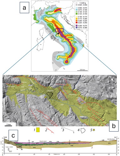
Figure 1. (a) Map of the seismic hazard of Italy, showing peak ground accelerations (g) that have a 10% chance of being exceeded in 50 yr (Meletti and Montaldo, 2007). The arrow refers to L’Aquila area. (b) L’Aquila area simplified geological map and (c) geological section. (1) Quaternary detrital deposit of the Middle Aterno R. intermontane basin (ASB: L’Aquila-Scoppito Basin; PSC: Paganica-San Demetrio-Castelnuovo Basin sensu (Nocentini et al. 2017, 2018); (2) Main Quaternary active faults; SPF: Scoppito-Preturo fault; PTF: Mt. Pettino fault; CFCFS: Colle Cerasitto-Campo Felice-Ovindoli fault system; BF: Bazzano-Fossa fault; PSDFS: Paganica-San Demetrio fault system; (3) geological section of panel b; (4) the studied area: L’Aquila historic downtown located inside the medieval walls perimeter (LAHC); (5) April 6, 2009 Mw: 6.29 L’Aquila earthquake epicenter; (b) geological section from Nocentini et al. (2017). ATF – Aterno Synthem (Holocene): mixed fine- and coarse-grained alluvial deposit; COL: colluvium; PPF – Ponte Peschio Synthem (Upper Pleistocene): coarse-grained alluvial deposit; LAB – Colle Macchione-L'Aquila Synthem (upper Middle Pleistocene): calcareous breccia; FGS – Fosso Genzano Synthem (Middle Pleistocene): coarse-grained alluvial deposit; MDS- Madonna della Strada Synthem (Calabrian): fine grained alluvial deposit; CCF – Colle Cantaro-Cave Formation (upper Piacentian-Gelasian): coarse-grained alluvial deposit; SYN: Neogene syn-orogenic formations sandstone and pelite; SLB: Meso-Cenozoic carbonate formations.

1.1. Geological setting

The study area is located in the western portion of Middle Aterno R. intermontane basin, which formed during the Plio-Quaternary extensional regime that affected the Central Apennines (Cavinato et al. 2002; Boncio et al. 2004; Cosentino et al. 2017). This region is characterized by a fold-and-thrust chain which accommodated crustal shortening. The post-orogenic extension led to the formation of a network of intermontane basins situated on the hanging wall of normal fault structures, oriented NW-SE and N-S (Cosentino et al. 2010). These basins are mainly filled by Quaternary continental detrital deposits pertaining to slope, lacustrine and alluvial environments, which reach up to several hundreds of meters in thickness. Within this context lies the Middle Aterno R. basin, bordered by SW-dipping normal faults, which are responsible for historical and current seismic activity (Galli et al. 2010; Storti et al. 2013). This basin consists mainly of two partially interconnected secondary basins: the L'Aquila – Scoppito basin (ASB) and the Paganica-San Demetrio-Castelnuovo basin (PSC) (Giaccio et al. 2012; Spadi et al. 2016; Cosentino et al. 2017; Nocentini et al. 2017; 2018), as shown in Figure 1b. The ABS, where the study area is located, is a half-graben filled with approximately 600 meters of continental deposits (Giaccio et al. 2012; Mancini et al. 2012; Nocentini et al. 2017; Tallini et al. 2019), characterized by complex stratigraphic relationships. It overlies the substrate formed by the pre-orogenic Meso-Cenozoic marine carbonate succession and the syn-orogenic upper Miocene terrigenous deposits (Tallini et al. 2019).

During the Piacenzian to Gelasian age, the carbonate sedimentation in the ASB comprises the deposition of S. Demetrio-Colle Cantaro (CCF) system (Spadi et al. 2016; Cosentino et al. 2017; Nocentini et al. 2017; 2018), composed of heterometric breccias with a clayey-silty matrix. The CCF system and the underlying bedrock are unconformably overlain by the sands and clays of the Madonna della Strada formation (MDS). The MDS represents the development of a fluvial environment with alluvial plains and extensive marshy areas near meandering river channels during the Early Pleistocene (Agostini et al. 2012; Storti et al. 2013). The Fosso di Genzano unit, incised into the earlier deposits or meso-Cenozoic bedrock, is primarily associated with distal portions of alluvial fans, which pass laterally to braided alluvial plains during the Middle Pleistocene.

Above these deposits, there are 20–100 m of LAB (Tallini et al. 2020). LAB consists mainly of heterometric carbonate clasts with sizes ranging from centimeters to meters, poorly sorted, and set within a sandy-clayey calcareous matrix that can vary in color from white to yellowish. Covering the top of the LAB are the RS, which formed during a humid and warm interglacial phase of the Late Pleistocene (MIS 5e, Eemian). These red clays include paleosols and epikarst deposits and exhibit highly variable thickness, reaching up to 30 m (Magaldi and Tallini 2000; Tallini et al. 2006). The LAHC buildings lay chiefly on LAB and RS.

Lastly, the uppermost deposits that have filled the ASB consist of fluvial deposits of the Fosso Vetoio system (FVS) (T1 – Early Upper Pleistocene), slope deposits of the Colle di Pile system (CPB) (Late Upper Pleistocene), Holocene colluvial deposits, and alluvial deposits of the Aterno River (ATF).

In Figure 1c a schematic geological section of ASB from (Nocentini et al. 2017, 2018) is provided.

2. Materials and methods

2.1. Multi-satellite A-DInSAR displacement data

In this research, we harnessed the power of Advanced Differential Synthetic Aperture Radar Interferometry (A-DInSAR) technique (Hanssen 2001) to investigate the historical ground displacement (or deformation) rates within the L'Aquila municipality. A-DInSAR relies on analyzing the phase differences between two radar satellite observations of the same location. These Synthetic Aperture Radar (SAR) images are analyzed to detect variations in the radar signal phase reflected from the Earth’s surface. These phase changes directly correlate with surface deformations, enabling the creation of precise high-resolution deformation maps (Wang et al. 2024). The A-DInSAR technique is increasingly being employed to study the temporal evolution of ground displacements using time series, particularly for objects with consistent reflectivity over time, referred to as Persistent Scatterers (PS) (Ferretti et al. 2001). A thorough and recent review about such methods is provided by Wang et al. (2024).

The PS-InSAR technique extracts information from a collection of SAR satellite images, forming an interferometric stack that enables the derivation of deformation patterns. We utilized datasets from two active satellite SAR missions, namely Sentinel-1 (by ESA) and Cosmo-SkyMed (by ASI), both offering historical archive data for scientific research. These datasets differ in terms of resolution, both spatial and temporal, as well as in acquisition bandwidth (C- and X-bands respectively). Sentinel-1 (S1) boasts a pixel resolution of 5 × 20 m on the ground, whereas Cosmo-SkyMed (CSK) offers a resolution of 3 × 3 m (specifically for the Interferometric Wide images available in the archive). The revisit time of the S1 constellation is shorter than that of CSK. The former operates with a revisit time of approximately 6 days, while the latter has an average revisit time of 16 days. This distinction is due to CSK's dual-purpose mission for both civilian and military applications, and it may result in sporadic gaps in data availability.

For this study area, we had to use two different satellite constellation datasets because in the CSK archive, there was a significant lack of images that would have made the multi-temporal analysis less valid. The datasets were processed using the PS approach (Kampes 2006) based on a total of 547 SAR images. The selected time frame spans from 2010 to 2022 for both ascending and descending orbital geometries:

Ascending orbital geometry: 386 images in Single Look Complex (SLC) format acquired by the Sentinel-1 (S1) satellites from 20 October 2014 to 03 August 2022.

Descending orbital geometry: 161 Single Look Complex (SLC) format images obtained by Cosmo-SkyMed satellites from April 14, 2010, to November 30, 2021.

Such kind of data was not available for any time ranges before the 2009 L’Aquila seismic event.

For each geometry, we carried out two separate post-processing analyses. A master image was chosen as the reference for calculating phase differences in other images within the dataset. The deformation rate values (expressed in mm/year) estimated by the A-DInSAR analysis were relative to the selected reference point. Additionally, we calibrated and validated our analyses using displacement data obtained from GNSS stations. Notably, the higher ground resolution of Cosmo-SkyMed SAR images resulted in a denser coverage of PS compared to the Sentinel-1 products.

The InSAR method used is the Persistent Scatterer Interferometry (PSI) Technique, according to the Kampes approach (Kampes 2006), with a single master baseline configuration, point selection criterion with amplitude dispersion analysis and linear deformation model in time.

The PS-ToolBox Suite within QGIS, developed by NHAZCA S.r.l. (NHAZCA PS Toolbox 2023) was employed for post-processing. Within this suite, we primarily utilized the time series visualization tool to understand the temporal evolution of deformation and the following two main post-processing analysis: Spatialization and Data Fusion.

Spatialization is a tool that enables the spatial conversion of point data into continuous maps through interpolation. The choice of the interpolation method was mainly based on the following criteria: (i) low computational burden, (ii) return of appropriately smoothed surfaces and (iii) minimization of assumptions regarding the data statistical distribution. With reference to point (iii), Sciortino et al. (2024) highlighted that the spatial distribution of PSs average vertical velocities, detected by Cosmo-SkyMed, cannot be assimilated to a simple spatial stochastic process, as the variogram of such data does not follow the most common geostatistical models. Therefore, interpolation methods such as Kriging, or similar, are not suitable for this kind of data. Interpolation according to the inverse of the distance, raised to a suitable exponent (e.g. 1 or 2, are the most widely used values), satisfies the three criteria mentioned above. Since the data present marked local spatial heterogeneities, which we are not interested in, in this study (but which may be the subject of future studies), the use of an exponent that provides a good smoothing degree would be preferable.

Therefore, the interpolation methodology used is based on the Inverse Distance Weighting (IDW) algorithm (i.e. with exponent equal to 1), which directly generates spatially continuous velocity or deformation maps. The algorithm calculates velocity or deformation values at each point in space by calculating a weighted average that accounts for both the distance of PS points from the point of interest and other relevant qualitative parameters. The formula used to estimate the value at a point P is expressed as: $$\mathit{\text{Vp}}={\displaystyle \sum \mathit{\text{Vi}}\ast (\mathit{\text{Pi di}})}/{\displaystyle \sum (\mathit{\text{Pi di}})}$$ where Vp is the value at point P, Vi is the value of measurement point i within the influence radius, Pi is the weight of each measurement point within the radius, and di represents the distance of measurement point i within the influence radius from the interpolation point.

Data Fusion is a tool that allows the merging of data from multiple satellites and their decomposition into vertical and horizontal directions using Line of Sight (LOS) data as a starting point. To enhance the reliability and spatial coverage of deformation information, we combined the data from Sentinel-1 and Cosmo-SkyMed. This approach leverages measurements from multiple sources with distinct orbital geometries and employs the strain tensor method (Guglielmino et al. 2011) through the ESISTEM (Extended Simultaneous and Integrated Strain Tensor Estimation from Geodetic and Satellite Deformation Measurements) (Guglielmino et al. 2010) method to create synthetic datasets incorporating multi-band information. The estimated displacement (DLOSkXp) for each synthetic data point (Xp=(xp,yp)) along the Line of Sight (LOS) is formulated using a first-order Taylor polynomial: $$D_{\mathit{\text{LOS}}}^k\left({\mathit{\text{XS}}}_d\right)=D_{\mathit{\text{LOS}}}^k\left(X_p\right)+{\nabla D}_{\mathit{\text{LOS}}}^k\left(X_p\right)\Delta {\mathit{\text{XS}}}_d$$

Here, Sd represents the direction cosine of the LOS, while ΔXSd contains the relative distances between the components of XSd points and the synthetic point Xp. The data fusion formulation takes into account two parameters: the maximum distance used for selecting nearby PS measurements to estimate deformations and the locality factor that weights each measurement’s contribution based on its distance from the point being estimated. The synthetic datasets for Up-Down and East-West components are then derived into a regular grid of squared cells from the vector decomposition of the deformation map along the multi-satellite LOS.

We point out here that the quality of the data set from Sentinel-1 is lower than that of the data from Cosmo-SkyMed and, therefore, its individual analysis has little convenience. The main advantage in the joint use of these two data sets consists in enabling to measure the horizontal and vertical components of the displacement vectors associated with the PSs in the monitored territory.

In a previous study (Sciortino et al. 2024), carried out on the same area and with an analogous data set, it was explained that thanks to the densely urbanized are with high backscattering quality and the extended revisit time of approximately 10 years provided by COSMO-SkyMed, we were able to extract a wealth of information from our results. This refinement has led to a scale reduction in the deformation rates of PSs, resulting in an instrumental error of approximately 0.3 mm/year. Moreover, an appropriate statistical treatment of data can further reduce noise and random errors contained in the time series (Sciortino et al. 2024).

For the study of A-DInSAR maps, the starting point was the identification of all factors that can cause ground deformation. For this purpose, recent papers were taking into account and a geomorphological and hydrogeological study was carried out through the analysis of a digital terrain model (DEM) and the piezometric level.

2.2. Collection and processing of geological – geomorphological, hydrogeological and geophysical data

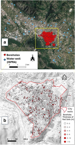
To characterize the study area geological and seismic features, we compiled all relevant geological, hydrogeological and geophysical data. A total of 142 Shear Wave Velocity (Vs) in-situ measurements, pertaining to the shallow lithologies within LAHC, also acquired from neighboring areas, were compiled from bibliographic sources (Lanzo et al. 2011; Del Monaco et al. 2013; di Giulio et al. 2014; Amoroso et al. 2018; Macerola et al. 2019; Amanti et al. 2020; Pagliaroli et al. 2020). We integrated with geological data from the literature (Nocentini et al. 2017; Antonielli et al. 2020), the log from an extensive dataset of 573 boreholes, many of which were drilled after the 2009 earthquake to facilitate the reconstruction of LAHC buildings, to carry out a comprehensive site geology analysis. In Figure 2a, the location of the 573 boreholes and 54 water wells acquired from the ISPRA (Istituto Superiore per la Protezione e la Ricerca Ambientale) database and used in this study is shown.

Figure 2. (a) Database of 573 boreholes (in red) from USRA (Ufficio Speciale per la Ricostruzione dell’Aquila) and 54 water wells from ISPRA (Istituto Superiore per la Protezione e la Ricerca Ambientale) database; (b) 573 boreholes classified with RS thickness.

The collected data formed a substantial database that enabled various GIS (Geographical Information Sistem)-based analyses and processing, aimed to redefine the surface geology with high accuracy and to determine the RS thickness. Due to their high compressibility, RS have been recognized in various previous studies as lithology responsible for site-specific seismic amplifications (Martelli et al. 2012; Del Monaco et al. 2013; Durante et al. 2017; Nocentini et al. 2017; Amoroso et al. 2018; Mannella et al. 2019; Tallini et al. 2020).

The produced geological map was rasterized, by assigning a Vs (shear wave velocity) value to each lithology based on literature data from Downhole (DH) and Multichannel Analysis of Surface Waves (MASW in situ measurements (Del Monaco et al. 2013; Amoroso et al. 2018; Macerola et al. 2019; Amanti et al. 2020; di Giulio et al. 2014; Lanzo et al. 2011; Pagliaroli et al. 2020). Quartiles (first, second, and third quartiles) were calculated for the collected Vs values.

Quartiles are statistical values that divide an ordered dataset into four equal parts. They are widely used to analyze the distribution of a dataset and identify variability within it. The three main quartiles are:

• First Quartile (Q1): This value divides the lowest 25% of the data from the remaining 75% of the higher data. It indicates the point where 25% of the data is below, and 75% of the data is above.

• Second Quartile (Q2) or Median: This value divides the dataset into two equal parts, with 50% of the data below and 50% of the data above. It is the central value of the distribution.

• Third Quartile (Q3): This value divides the lowest 75% of the data from the top 25% of the data. It indicates the point where 75% of the data is below, and 25% of the data is above.

Quartiles are useful statistical tools for understanding the distribution and variability of data in a numeric dataset.

The assigned Vs value to the lithologies is the median (Q2).

Values of the RS thickness, as well as the groundwater level, were interpolated according to the same above discussed criterion utilized for spatializing InSAR data, i.e. the Inverse Distance Weighted (IDW) method. The result of these interpolations is two raster, depicting the variation of the RS thickness and piezometric level across the entire area within the city medieval walls.

A Digital Elevation Model (DEM) with a 5-meter resolution became necessary for assessing the elevation differences and calculating slopes. This was achieved using the dedicated "Slope" analysis algorithm available in the open-source software QGIS. Furthermore, through a subtraction operation between DEM and the groundwater elevation raster, carried out using raster calculator, it was possible to estimate the depth of the water table relative to the ground surface.

2.3. Calculation of the Pearson correlation coefficient

The PCC, often denoted as "r," is a statistical measure used to assess the linear relationship between two variables. It measures the strength and direction of the relationship between two continuous variables.

The formula to calculate the Pearson correlation coefficient (r) is as follows: $$r=\frac{\sum \left[\left(X_i-\overline{X}\right)\left(Y_i-\overline{Y}\right)\right]}{\sqrt{\sum {\left(X_i-\overline{X}\right)}^2\sum {\left(Y_i-\overline{Y}\right)}^2}}$$ where:

$r$ is the Pearson correlation coefficient, $\mathit{\text{Xi}}$ and $\mathit{\text{Yi}}$ represent each value respectively in the first and second dataset, $\overline{X} \mathrm{\text{and}} \overline{Y}$ are the mean of values respectively in the first and second dataset.

The PCC takes values between −1 and +1

$r=1$ indicates a perfect positive correlation (when one variable increases, the other increases linearly)

$r=-1$ indicates a perfect negative correlation (when one variable increases, the other decreases linearly)

$r=0$ indicates no linear correlation (the variables are not linearly related)

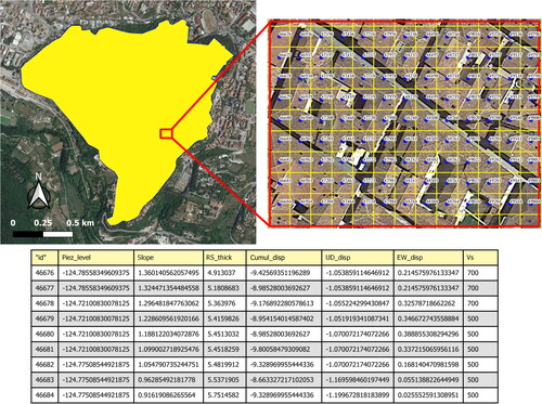
To calculate PCC between PF and SAR deformation, it was necessary to create a grid with a 10 m x 10 m mesh and spatialize data, in order to create continuous surfaces that were sampled at the centroids of each grid cell (Figure 3). In this way, each pixel was assigned a value for cumulative and vertical displacement, ground slope, RS thickness, piezometric level and Vs.

Figure 3. On the top is the 10 m × 10 m grid covering the entire historic center within the medieval city walls, which was used to sample the rasters for correlation purposes. Below, the table displays the values for each grid centroid, including piezometric level, RS thickness, terrain slope, cumulative vertical and horizontal displacement, and Vs of the outcropping lithologies.

2.4. Analysis of seasonal ground movements and correlation with meteorological data

Groundwater level variations, associated with seasonal precipitation changes, lead to modifications in pore pressure in the soil/rock column underlying the studied area. Therefore, we expect to observe a correlation between seasonal variations in subsidence velocities and rainfall intensity values. In order to study such correlation, we used precipitation data provided by NASA (NASA POWER Data Access Viewer 2023), in the form of daily and monthly time series. Both meteorological and subsidence data were preliminarily processed.

The time series of PS cumulative displacement values utilized here consist of an array in which each value is given by the average displacement of all PSs, located on the ground, in a certain time. To remove the effect of seasonal thermal strain of buildings on the measured vertical ground displacements, the PSs located on buildings have been excluded from this analysis. Such time series have been analyzed by means of a detrended approach, as data show an evident multi-year trend. To remove the effects of non-climatic factors, thus isolating seasonal variations, the oscillations of values compared to the long-term trend were considered. In particular, the deviations, or residuals, compared to a linear trend were considered. These deviations were then standardized as follows: $$s=\left(r_e–\text{m}\right)/\sigma$$ where, s represents the standardized residual, r_e the values of the residuals, m and σ, respectively, their mean and standard deviation, calculated over the studied time range. Standardization transforms the data into dimensionless units, allowing comparison between different data types (such as rain intensity and cumulated deformations).

As regards the precipitation data, quarterly averages were calculated from daily intensity values. Each value represents the average rainfall intensity over the preceding three months. By way of example, the May quarterly average is equal to the average of daily intensities of March, April, and May. These values were also standardized according to the aforementioned formula, considering the residuals with respect to a horizontal trend (i.e. compared to the average value of the whole series). Since only the water that actually infiltrates the ground contributes to aquifer recharge, the daily data was preliminarily further corrected, according to a very simple model that accounts for runoff during intense rainfall events. To achieve a first approximation estimate of the infiltration-runoff proportion, the following simple linear model with saturation was utilized: $$\text{p}=\text{i},\text{for i}<={\text{i}}_{\text{tr}};$$ $$\text{p}={\text{i}}_{\text{tr}},\text{for i}>{\text{i}}_{\text{tr}};$$ where p denotes the flow rate per m² of infiltrated water, i the rainfall intensity and i_tr an appropriate threshold value to be determined. Namely, according to this model, when the intensity is lower than the threshold value, all the rainwater infiltrates. When the intensity exceeds the threshold value i_tr, only the quantity equal to i_tr infiltrates, whereas the excess forms runoff water. Based on these corrected intensity values, quarterly averages were calculated.

Then, the cross-correlation was carried out between time series of corrected standardized precipitation intensity and average monthly cumulative displacement of all ground PSs, for the entire monitoring period (from April 2010 to November 2021). The unknown variables to be determined through this analysis were the i_tr threshold value and the time shift between the two series. These values were determined by finding the pair of values, in the (i_tr, shift) plane that maximized the correlation between the two considered time series, i.e. those for which the correlation (in absolute value) between precipitation and cumulative displacement values, reaches its maximum.

3. Results

The A-DInSAR map, obtained from Cosmo-SkyMed images acquired between April 2010 and November 2021 in the descending orbit, reveals more pronounced deformations in the south and southwest LAHC. In Figure 4a, the interferometric data has been interpolated to spatialize the deformation over the study area, and from this map, areas characterized by deformation of more than −1 mm/year have been extracted. Points P1 and P2 exemplify the contrasting deformation trends for PSs in the eastern-northeastern and southern-southwestern sectors of LAHC, respectively. Deformations recorded along the satellite’s Line of Sight (LOS) exhibit significant variation from north to south, ranging from no deformation to a cumulative displacement exceeding −25 mm over an 11-year period. In the map depicted in Figure 4a, stable areas are shown in green, while areas moving away from the satellite are indicated by colors ranging from yellow to orange.

Figure 4. (a) A-DInSAR Map obtained from Cosmo-SkyMed images acquired between 2010 and 2021 in the descending orbit and interpolated to spatialize the deformation. Stable areas are shown in green, while areas moving away from the satellite are indicated by colors ranging from yellow to orange. Black line indicates areas characterized by more pronounced deformation (more than −1 mm/year). Blue points (P1 and P2) are two PSs used for illustrating deformation trend in Northern and Southern sector of the study area; (b) vertical and horizontal A-DInSAR map obtained from the data fusion between COSMO-SkyMed descending April 2010–November 2021 and Sentinel-1 ascending October 2014–August 2022 images.

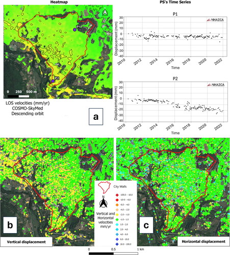
3.1. Horizontal and vertical deformation of L’Aquila hill

The results of decomposing the deformation into horizontal and vertical components, are depicted in the maps in Figure 4b and c which use the same color scale as Figure 4a, to represent vertical and horizontal PSs deformation rates. In the vertical deformation map, warm colors indicate PSs experiencing subsidence (i.e. those with negative velocity, moving away the satellite), while cool colors represent points exhibiting uplift (i.e. with positive velocity, approaching to satellite). As for the horizontal deformation map, PS with negative velocity (ranging from yellow to red) are associated with westward movement, while those with positive velocity (ranging from cyan to blue) indicate eastward movement. In both maps, points with mild deformations falling within the range of −1 to 1 mm/year are represented in green.

From the maps in Figure 4, it can be observed that subsidence is distributed across the entire study area, with a more pronounced character in the southwestern LAHC sector. In contrast, horizontal displacement is characteristic of a smaller number of PS and does not exhibit a preferred direction. For this reason, the horizontal deformation map in calculating the PCC has not been used.

3.2. Identification of factors predisposing deformation

To unravel the causes of the ground deformations, we first identified the geological and geomorphological factors that can possibly influence them. We carried out a detailed analysis of the central area of L'Aquila (LAHC) within the medieval walls, which is the focus area for our study.

A careful review of the existing literature points out that the geological characteristics of the substrate upon which the L'Aquila’s buildings are constructed can be responsible for various seismic amplification effects (Martelli et al. 2012; Del Monaco et al. 2013; Durante et al. 2017; Nocentini et al. 2017; Amoroso et al. 2018; Mannella et al. 2019; Tallini et al. 2020). In other words, the nature of the rocks and sediments exposed in the study area can have a significant impact on seismic amplification. Based on a geomorphological and hydrogeological analysis, four predisposing factors (PFs) potentially influencing deformations were selected:

• thickness of the Red Soils (RS);

• surface lithology;

• terrain slope;

• water table depth

In considering surface lithology, it is worth noting that only lithology with a minimum thickness of 2 m has been mapped.

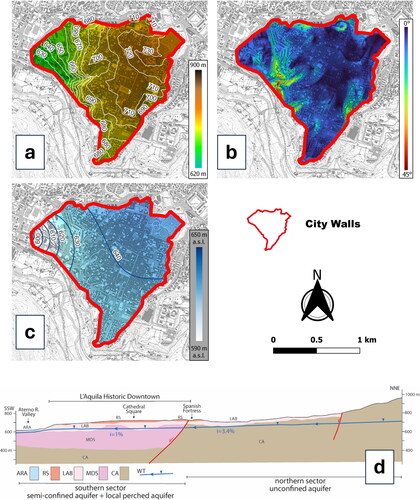
The study area occupies a flat-topped hill with elevations ranging from 628 m a.s.l. to 736 m a.s.l. (Figure 5a). A difference in elevation of over 100 meters in 2 km² is accommodated by areas with potentially steep slopes (Figure 5b), a characteristic that can influence deformations. The multilayer porous aquifer of the intermontane plain, in which is located LAHC, constituted by the Quaternary detrital formations, may be represented hydrogeologically with a unique reference water table with centripetal groundwater flowpaths. This aquifer is dominantly recharged by the surrounding carbonate reliefs acting as regional aquifer (Petitta and Tallini 2003). By observing the section of Figure 5d, the carbonate aquifer outcrops in the northern sector, while it is mainly buried in the southern one by the Quaternary formation (LAB and MDS). The coarse-grained L’Aquila Breccia (LAB) and low-permeability fine-grained MDS formation act as local aquifer and aquitard respectively. In the northern sector the carbonate aquifer is unconfined because only the LAB aquifer overlays on top on it with a negligible thickness, while in the southern one the carbonate aquifer is semi-confined due to the overlaying on it of the MDS aquitard with a considerable thickness of 200–400 m. Moreover, in the southern sector, LAB behaves as a local perched aquifer and overlays the MDS formation so that LAB feeds minor springs in the southern slope of L’Aquila hill (Hanssen 2001) (Figure 5d). The water table varies from West to East between 590 and 640 m a.s.l. with the groundwater flowing towards the SE (Figure 5c). It is shallower in the W part of the city and deeper in the NE (Figure 5). MDS aquitard plays an important role in the LAHC hydrogeological setting because it, as well as being groundwater saturated, partly confines laterally the regional carbonate aquifer.

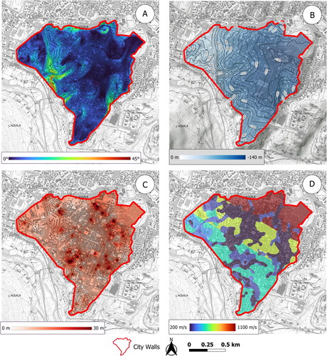
Figure 5. (a) Ground elevation (m a.s.l.); (b) terrain slope (°); (c) water table (m a.s.l.); (d) LAHC hydrogeological section. ARA: Aterno River alluvium, gravel, sand, silt (local aquifer); RS: Red Soil (local aquiclude-aquitard); LAB: L’Aquila Breccia, gravel and breccia mixed with sand and silt (local aquifer); MDS: Madonna della Strada Formation, clayey silt and sand (aquitard); CA: carbonate aquifer; WT: water table; i: hydraulic gradient.

Several studies (Del Monaco et al. 2013; Durante et al. 2017; Nocentini et al. 2017; Amoroso et al. 2018; Mannella et al. 2019) suggest that the varying amplification effects recorded on LAHC buildings during the 2009 earthquake may be associated with the extreme variability in terms of thickness and lithology of the continental deposits, filling the Plio-Quaternary graben upon which the city was built. In particular, (Del Monaco et al. 2013; Durante et al. 2017; Amoroso et al. 2018; Mannella et al. 2019) considered the RS as a key factor in the distribution of deformation and observed damage intensity. Tallini et al. (2020) recognized, through an analysis of HVSR microtremor data, a peak in the mid-frequency microtremor range (f1, 3–13 Hz), partly related to the variation of RS thickness and areal distribution. In terms of seismic amplification, this peak can result in seismic coupling between the frequencies of shallow lithologies and the fundamental frequency of buildings. The authors estimated that 80% of the buildings severely damaged or destroyed by the 2009 earthquake could experience such seismic coupling.

In this context, it is necessary to redefine the LAHC geological map with such detail that it allows for an analysis of deformations at the scale of individual buildings. Indeed, the high number of PSs in the study area and the resolution of SAR images enable us to extend the analysis to a large scale.

3.3. Borehole stratigraphy and redefinition of geological mapping

We utilized data from 573 boreholes within LAHC (Figure 2b), archived in the USRA database (USRA), to produce a highly detailed geological map that accurately reflects the variations in lithology across the study area. This map was primarily used to characterize the spatial variability of the Red Soil (RS) thickness.

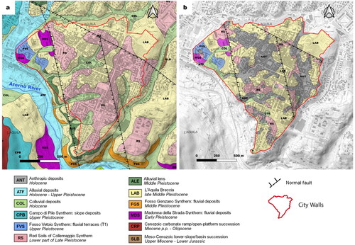
By integrating borehole stratigraphy with literature data mentioned above, we produced the geological map in Figure 6b, which, compared to the map (Nocentini et al. 2017) (Figure 6a), provides a higher level of detail, allowing for an accurate comparison between geological data and A-DInSAR deformations. The key improvements in the new map are: mapping anthropic deposits (ANT) exceeding 2 meters in thickness across all relevant areas; significant reduction of the RS extent based solely on borehole encounters. It’s worth noting that the new map is limited to the medieval city wall, the focus of this study (LAHC).

Figure 6. (a) Geological map modified from Nocentini et al. (2017); (b) new detailed geological map resulting from the analysis of 573 boreholes database and literature data.

Therefore, starting from the new geological map, we selected some representative PSs located on RS and exposed LAB, and analyzed their time series.

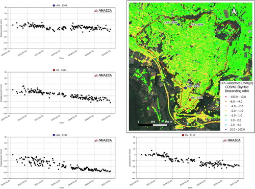
In the A-DInSAR LOS map created with descending Cosmo-SkyMed images, shown in Figure 7, the blue dots indicate the location of measurement points positioned on LAB, while the red dots represent those on RS. The scatterers for which time series are provided are located near boreholes S566, S544, S339, and S110. The time series of PSs located on RS reveal the presence of similar LOS deformations in different areas of LAHC, with cumulative displacement values reaching −20 mm. Conversely, the time series of the two PS points located on LAB highlight a significant difference in deformation behavior. In the northern sector, where S566 is located, deformations are mild, with a cumulative displacement value of approximately −5 mm over 11 years. On the contrary, borehole S339, situated southwest of LAHC, exhibits very pronounced deformations, with a cumulative displacement of −28 mm.

Figure 7. Time series Cosmo-SkyMed descending PSs located on LAB (blue dots) and RS (red dots). In the A-DInSAR LOS descending orbital geometry map green PSs are considered as stable; yellow-red PSs are moving away from the satellite; cyan-blue PSs are moving toward the satellite.

3.4. Geophysical data – Vs

Once the LAHC geology was redefined, it was necessary to assign a numerical value to each outcropping lithology for calculating the correlation between satellite-detected deformations and geology. To this aim, we used seismic shear wave velocity (Vs) values from literature data (Lanzo et al. 2011; Del Monaco et al. 2013; di Giulio et al. 2014; Amoroso et al. 2018; Macerola et al. 2019; Amanti et al. 2020; Pagliaroli et al. 2020).

The quartile values Q₁, Q₂, and Q₃, calculated for each lithology based on the Vs data are illustrated in Table 1 and by the boxplot in Figure 8a. Quartiles provide information about data dispersion and can be used to identify any significant features in value distribution. The boxplot in Figure 8a outlines the large variability of Vs values within LAB, with values ranging from 200 to 1200 m/s. The histogram in Figure 8b further details this distribution, dividing the Vs values of LAB into three intervals marked by red dashed lines.

Figure 8. (a) Boxplot of Vs data (summarized in Table 1) which shows high variability of LAB Vs values, ranging from 200 to 1200 m/s; (b) distribution of Vs values (number of values). The dashed red lines separate the Vs of the LAB into three intervals; (c) boxplot of Vs data considering the classification of LAB presented in Table 2; (d) geological map with an internal division of LAB based on the abundance of the muddy-limestone matrix. From LAB 1 to LAB 3 the silt fraction increases and the Vs decreases (cfr. Table 2).

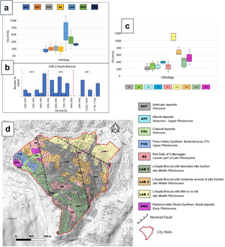
Table 1. Q₁, Q₂, and Q₃ calculated based on the Vs literature data for each outcropping lithology.

Lithology	Q1	Q2	Q3
ANT	167.5	200	250
ATF	230	275	300
COL	200	300	320
RS	180	265	300
LAB	500	700	1000
MDS	400	500	600
FVS	364.25	390	400

For this reason, through a careful analysis of borehole stratigraphy and the lithological characteristics of the LAB in LAHC, we divided LAB into three categories based on the abundance of the fine-grained fraction. In the southern sector, LAB with a significant silty fraction is exposed (LAB 3), to which Vs values ranging from 200 to 500 m/s have been associated. In the central zone of LAHC, the amount of silt within the LAB decreases, and the Vs values rise to 500–800 m/s (LAB 2). Finally, in the northern and northeastern sectors, the silty fraction is almost absent, and the Vs values are higher, ranging from 950 to 1200 m/s (LAB 1). This internal division within LAB is depicted in the geological map in Figure 8d, while Table 2 presents the Vs values (Q₁, Q₂, and Q₃) calculated for each outcropping lithology, based on the distinction of LAB into three categories, along with the associated VS/lithology boxplot (Figure 8c). In Table 2 is also reported the number of Vs measurement used in calculation of Vs median (Q₂).

Table 2. Vs values (Q1, Q2, Q3) calculated for each outcropping lithology, based on the distinction of LAB into three categories (LAB 1, LAB 2, LAB 3).

Unit	Number of Vs Data	Q1 (m/s)	Q2 (m/s)	Q3 (m/s)
ANT	16	167,5	200	250
COL	25	200	300	320
ATF	11	230	275	300
FVS	6	364,25	390	400
RS	10	180	265	300
LAB 1	11	1000	1100	1200
LAB 2	17	600	700	750
LAB 3	13	400	500	500
MDS	35	400	500	600

3.5. Calculation of Pearson’s correlation coefficient (PCC)

We verified the relationship between geological-geomorphological and hydrogeological PF, represented in Figure 9, and deformation in LAHC, by means of PCC estimates. We compared the cumulative deformation (evaluated by interpolation of Cosmo-SkyMed descending velocity values) and vertical deformation (evaluated by interpolation of velocity values resulting from the decomposition of velocities calculated by combining Cosmo-SkyMed descending and Sentinel-1 ascending) with slope maps, RS thickness, depth of regional aquifer and the Vs of the outcropping geology.

Figure 9. geological-geomorphological and hydrogeological predisposing factors (PF): (a) ground slope (°); (b) RS thickness (m); (c) water table depth (m below ground level); (d) Vs (m/s) of the outcropping lithologies.

Table 3 shows the results obtained from the correlation between cumulative and vertical deformation, and PF.

Table 3. Person coefficient values related to correlation between cumulative displacement and the considered predisposing factors, as well as between these and vertical PS velocity.

Predisposing factors	Cumulative displacement (mm)	Vertical displacement (mm/a)
Depth of regional aquifer	−0.394609509	−0.521570082
Ground slope	−0.211930302	−0.223682426
Red Soils thickness	0.179659561	0.12674804
Vs of outcropping geology	0.467233498	0.459702848

We point out here that that the primary aim of this study is to identify predisposing factors that exhibit statistically significant correlations, supporting the hypothesis that these factors influence subsidence rates. A more detailed quantitative analysis, such as multivariate analysis involving all the PFs and dividing the study area into sectors with homogeneous structures (e.g. considering areas with different L'Aquila Breccias, LAB1, LAB2 and LAB3, as well as areas bounded by faults), is beyond the scope of this study and will be the subject of future research.

The Pearson correlation values observed (Table 3) are statistically significant. Suffice it to consider that, according to the well-known p-value approach, a correlation value equal to 0.126 (the lowest observed in Table 3) is statistically significant if the data set considered includes a number of data of the order of magnitude of one hundred, while our data set includes several tens/hundreds of thousands of values.

3.6. Correlation between subsidence fluctuations and precipitations

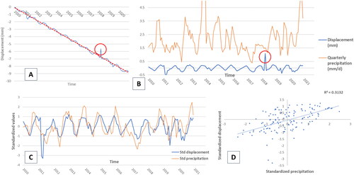
Figure 10a and b show the detrended time series of average deformations, representing the spatially averaged values across the study area. The y-axis values in Figure 10c represent the standardized deviations of the values in Figure 10b relative to the trendline. The orange curve represents the standardized values of quarterly precipitation. The Figure 10c shows the result of the cross-correlation analysis, involving the corrected and standardized precipitation values (see Section 2.4 in Methods), in which the runoff threshold precipitation and the temporal shift were estimated, by maximizing of the correlation coefficient. The optimal values of these unknowns were given by threshold rainfall intensity of 4.7 mm per day and zero shift (note, however, that the quarterly data is already delayed, as it is a moving average over three months). The July 2018 displacement standardized residual value (circled in red in Figure 10a and b) has been removed as it is a suspected outlier. Indeed, it presents the maximum positive deviation of the entire series in a period of the year in which the deviations are systematically negative. The two standardized time series of detrended PS displacement and quarterly precipitation exhibit a notable degree of history matching, thus highlighting a significant relationship between the seasonal variations in subsidence on the rainfall rates of the previous months. Figure 10d shows the linear regression, with the relative squared correlation coefficient, between the two considered time series. Each data point in Figure 10d represents a specific date, with the ordinate value corresponding to the standardized displacement measured on that date and the abscissa value corresponding to the standardized and corrected precipitation on the same date.

Figure 10. (a) Result of detrending the time series of average displacements (i.e. spatially averaged over the studied area); (b) values in ordinates in the diagram are given by the standardized deviations of the curve panel (a) compared to the trendline. The orange curve represents the values of quarterly precipitation; (c) curves of standardized values of ground deformation and precipitation and result of the cross-correlation analysis carried out by maximizing of the correlation value; (d) linear regression, with the relative squared correlation coefficient (R²), between the two considered time series.

4. Discussions

Several studies attribute the variations in seismic amplification observed in LAHC buildings during the 2009 and 1703 earthquakes to the significant differences in the characteristics of continental sediments filling the Plio-Quaternary graben underlying the city (Martelli et al. 2012; Del Monaco et al. 2013; Durante et al. 2017; Nocentini et al. 2017; Amoroso et al. 2018; Mannella et al. 2019; Tallini et al. 2020). Sciortino et al. (2024) observed a systematic increase in post-seismic subsidence rate, with increasing seismic damage (for both the 2009 and 1703 events), in the time range 2010-–2021. This study, through A-DInSAR analysis of Cosmo-SkyMed images acquired between 2010 and 2021, supports the notion that geological and hydrogeological conditions are key factors explaining the observed damage patterns. The PCC (Table 3) shows a positive correlation between satellite-detected ground deformations and the Vs values, whereas a negative correlation between the former and the depth of regional aquifer, is observed. In other words, lower Vs values correspond to greater InSAR deformation, and a deeper water table translates to less deformation (both subsidence and cumulative deformation along the LOS).

Decomposing PS velocities into H (horizontal) and V (vertical) components reveals subsidence dominant deformation feature in L'Aquila, indicating a primarily vertical displacement. Notably, the PCC between Vs and Cumulative Displacement and between Vs and Vertical Displacement is almost identical. Conversely, the water table depth exhibits an anticorrelation, with the highest PCC value observed in the case of vertical displacement rather than cumulative deformation.

To create a new and more precise geological map, we integrated site-specific geological and geophysical data from the literature. The collection of Vs measurements to associate with outcropping lithologies highlighted significant variability in LAB, whose lithological and textural differences had already been identified by Antonielli et al. (2020) but had not been represented in the LAHC geological maps until now. They recognized two different levels in LAB: a lower level with a massive structure and grain-supported, containing blocks ranging in size from decimeters to meters, which directly overlies the bedrock and predates Quaternary deposits; the upper level is mud-supported and contains smaller blocks ranging from centimeters to a few decimeters.

The LAB lithology in the northern area of LAHC appears competent (lithoid, with a sparse matrix), whereas the southern breccias are dominated by a silty fraction. The LAB outcropping in the central sector of LAHC represents a transitional zone with roughly 50% silty matrix and 50% clasts.

The observed variability in Vs values within LAB necessitated mapping of this internal lithological difference: in the northeast sector, more compact and lithoid breccias outcrop with a median Vs value of 1100 m/s. The Vs value decreases to 700 m/s in the central sector, where the lithology shows an increase in the silty matrix. Finally, the LABs outcroping in the southwest sector are characterized by the lowest Vs values, with a median of 500 m/s. Different Vs values in the breccias correspond to different ground deformation behaviors, which cannot be considered negligible for the purpose of correlating deformation and lithology. In fact, higher Vs values correspond to areas with less deformation, while the deformation of PS gradually increases southwestwards, where the cumulative displacement can reach up to −25 or −30 mm. This trend is confirmed by the PCC calculation, which has shown a moderately strong correlation between the Vs of outcropping lithologies and cumulative and vertical deformation.

The observed subsidence results from competing compaction phenomena of soil and rocks, at different depths and observation scales.

In Figure 11a PSs are grouped into the following cumulative deformation classes, appropriately chosen, with uplift; 0 − 0.3 mm; −0.3, −1 mm; −1, −7 mm; −7, −10 mm; < −10 mm. The comparison with Figure 8d shows a clear overlap: the gray points fall on LAB 3, the orange ones predominantly on LAB 2 and the yellow ones fall in an area delimited partly by a main fault and to the SE by the limit between LAB 1 and LAB 2. Therefore, subsidence values appear to be controlled by the kind of breccia. Only near the NE walls is there a small cluster of points showing subsidence tending towards zero or uplift.

Figure 11. (a) PSs grouped in cumulative displacement classes; black line and the associated, 50 m width, semi-transparent red strip is the trace section (panel b); (b) the comparison of deformation and subsurface geology is shown through the projection of the cumulative displacement values (mm) of the PSs falling in the red semi-transparent band (in panel a) and the geological section from (Antonielli et al. 2020); (c) the comparison of ground deformation and geology is shown through the superposition of the cumulative displacement and the geological section in panel b. Note the good matching between deformation with the Red Soil bottom boundary.

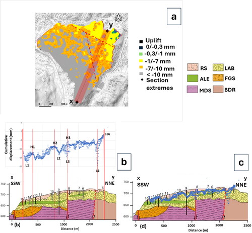
To facilitate a more accurate comparison of deformation data with the subsurface structure, Figure 11b illustrates the values associated with PSs falling within the a 50-meter-wide strip, marked in semi-transparent red in Figure 11a. This band surrounds an accurate geological section constructed by Antonielli et al. (2020), illustrated below in Figure 11b, with the same scale. It is highlighted that, although the areal distribution of the lithologies proposed in that article has been determined with greater accuracy in the present work, the geological section proposed by them can be considered reliable, being based on data from several wells well aligned with the section itself. Figure 11a and b (i.e. plan and section) point out that the subsidence decreases going from LAB 3 to LAB 2 and LAB 1. However, the local variations seem to be predominantly controlled by the RS, as the trend of the point cloud in the diagram faithfully follows the thickness of the RS units.

Local maxima H1 and H2 occur precisely in areas where the RS is thin or absent. The point cloud minima (i.e. maximum subsidence values) in the interval from L1 to L2 are found where the section displays the greatest RS thicknesses. The local minimum L4 (very high subsidence) is located near the fault, where the section shows an increase in RS thickness. This could be explained by the presence of more deformable fault rock and potentially greater erosion at the fault zone, or alternatively, due to sin-kinematic nature of RS, resulting in a thicker RS. The situation with maxima and minima H3 and L3 is a bit more complex. Figure 11a indicates that near the intersection between the geological section and the fault, points with that abscissa falling within the strip exhibit greater subsidence to the right of the section and lower values to the left. Therefore, maximum H3 is associated with the points on the left, whereas L3 corresponds to those on the right side. The geological section (Figure 11b) also shows an increase in RS near the fault. This might be because the fault brought materials with different mechanical properties and erosion susceptibilities into contact, resulting in further geological complexities. What is evident is the presence of significant anomalies in deformation values near the two faults. Furthermore, the maxima from H1 to H3, where RS is absent (or significantly thin), follow an increasing trend, likely associated with an increase in LAB thickness in that direction. On the other hand, the maxima in the segment between the two faults show an almost absent trend, with values around −5 mm, consistent with an almost constant LAB thickness. The maximum H4, where subsidence tends towards zero (and transforms into a slight uplift slightly further northeast outside the section), is found where the RS, as well as MDS units, are absent, and LAB 1 directly rests on the carbonate basement uplifted by the fault.

To compare the role of quaternary deposits in affecting ground deformations the cumulative displacement scatterplot of Figure 11b has been superposed over the geological section. Note the good matching between displacement with the Red Soil bottom boundary.

The results illustrated in Figure 11a–c confirm that a significant contribution to the observed subsidence phenomenon is provided by the consolidation of Quaternary units.

As the hydrogeological behaviour is controlled by lithology (for instance, the abundance of silty-clay matrix influences water filtration), the correlations between InSAR deformation and outcropping lithologies, as well as between InSAR deformation and water table depth, obtained through the calculation of the PCC, represent two sides of the same coin.

In granular soils, seismic shaking produces well-known phenomena of variation in porosity, such as compaction or dilatancy. In the case of saturated fine-grained soils (even above the water table, i.e. in soils saturated by capillarity) a first phase of porosity variation occurs slowly, associated with fluid expulsion (Terzaghi consolidation, Figure 12), followed by a second phase of secondary consolidation, due to creep phenomena (e.g. Lancellotta 2014). The time evolution of fluid discharge related consolidation in soil and rock depends on both their compressibility and permeability (Guerriero et al. 2021; Guerriero 2022). In unsaturated soils, the first compaction phase is immediate and is followed by secondary consolidation, which occurs slowly. Note that, as we only have post-seismic data, we cannot detect immediate consolidation effects in unsaturated soils. Therefore, the speed and deformation values of the monitored PS are given by the sum of effects of primary and/or secondary consolidation in saturated soils and the only secondary consolidation of non-saturated ones. Furthermore, large-scale movements of groundwater, involving the fractured carbonates of the basement, contribute to the observed subsidence phenomenon, as assessed by Moro et al. (2017).

Figure 12. Scheme of pore pressure dissipation during the co-seismic period of the 6 April 2009 Mw. 6.29 L’Aquila earthquake within above all the low permeability MDS formation and LAB3.

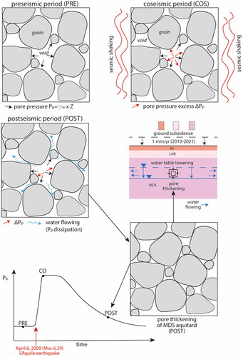
It is known that before a seismic event, the phenomenon of dilatancy occurs at the hanging wall of normal faults (Doglioni et al. 2013; Moro et al. 2017) caused by the opening of fractures and voids that, during the pre-seismic phase, draw groundwater downward, leading to a lowering of water table. Moro et al. (2017) carried out a large-scale InSAR analysis that demonstrated that in the months preceding the 2009 earthquake, near to the epicentral area, some of the basins filled with alluvial deposits experienced subsidence phenomena associated with the water table lowering of the Gran Sasso aquifer, to which they are connected. The migration of water from the multi-layer aquifers caused pre-seismic subsidence, while after the earthquake, uplift was recorded in the same areas.

Pore pressure variations can account for the observed fluctuations in the water table, a phenomenon often documented during earthquakes (Doglioni et al. 2013). In fact, during an earthquake, as the hanging wall of a normal fault subsides, interstitial fluids previously accumulated within dilated volumes are expelled. This prior migration of fluids had led to a gradual increase in pore pressure during the pre-seismic phase. However, with the expulsion of fluids from voids and fractures due to the hanging wall downward movement, pore pressure diminishes, subsequently causing a rise in the water table. The subsequent lowering of the water table to its natural level will occur more rapidly if filtration is favored, and more slowly if water has to pass through lithologies with a low permeability coefficient. The delayed dissipation of pore pressure in the MDS aquitard and LAB 3, low permeability lithologies, can explain the well-recognized negative correlation between subsidence and water table depth in the period following the 2009 earthquake (Figure 12).

Given the highly irregular spatial distribution of the RS, we believe it is indeed the content of silty matrix within LAB 3 (and secondarily within LAB 2) that accounts for the higher subsidence rate within the study area. This lithology, being both characterized by a low S-wave velocity and a low permeability coefficient, explains why the highest ground deformation values are localized in the southern and western areas of the city.

The seasonal cyclicity of precipitation was also taken into account with the goal to assess its potential influence on the monthly variations of InSAR deformations. With this aim, the cross-correlation of the quarterly average precipitation (mm/d) for each month from 2010 to 2021 with the average deformation of all PS resulting from the InSAR analysis using Cosmo-SkyMed descending images during the same period (mm/month), was analysed. In light of the explanations provided regarding interactions between water table oscillation and deformations – where a rise in the piezometric level corresponds to a decrease in the deformation rate – a significant correlation value has been identified, with PCC = 0.560 (i.e. R² = 0.313). This highlights a significant connection between the seasonal variations in subsidence on the rainfall rates of the previous months. To verify whether the fluctuations in the groundwater level, resulting from seasonal variations in precipitation, are the only ones responsible for the seasonal variations in the subsidence rate, an analysis carried on via geomechanical modeling would be needed, to quantify variations in effective stress in the subsoil. This kind of analysis is beyond the scope of the present study and will be the subject of future research.

In evaluating the obtained results, it is necessary to remember that reconstructing the outcropping geology in an urban setting is quite difficult, because of building and infrastructure covering, even when a rich database of site investigations is available. Therefore, the correlation value between cumulative displacement and Vs, as well as that with RS thickness, could be different if an even more detailed geological map were available. A 3D geological model of the subsurface would also allow for the assessment of the spatial variability, thickness, and Vs values of the lithologies on which the LAHC buildings are constructed in relation to the deformations detected by Remote Sensing data.

5. Conclusions

The correlation analysis between satellite and geophysical data represents a novel aspect that sheds light on the potential of interferometry. The satellite records a difference in deformation behavior as the Vs values of the outcropping lithology vary. Regarding the LAB, the satellite can even describe subtle internal variations in composition within the lithology, which are well-documented in the literature and supported by a high variability of Vs within this lithology.

The LAB classification based on the amount of silty matrix is the key to comprehending the decade-long deformation phenomena that characterize the historic center. The low permeability coefficient of LAB 3, and LAB 2 introduces a delay in the dissipation of pore pressure within these rocks. Notably, the presence of silty matrix inhibits filtration and hinders the decline of the water table. When seismic shaking occurs, the water – previously filling voids and fractures that formed at the fault’s hanging wall during the pre-seismic phase – is forcefully expelled, causing a rise in the water table. This model of delayed pore pressure dissipation also may elucidate the observed correlation between precipitation patterns (which induce seasonal water table variations) and monthly fluctuations in satellite-detected deformations.

The results illustrated in the present study integrate those achieved in a previous one (Sciortino et al. 2024), carried out on the same area and involving analogous InSAR data sets, which outline as greater post-seismic InSAR deformations correspond to more severe damage to buildings, both for 2009 and 1703 earthquake. Based on this evidence, use of long-term InSAR time series emerges as a promising tool aimed at mapping and characterizing high-risk seismic areas.

Author contributions

“Conceptualization, A.S., M.S., pm, V.G., M.T.; methodology, R.M., V.G., pm, A.S.; software, R.M, V.G.; validation, pm, M.T.; formal analysis investigation A.S., V.G.; data curation, R.M., V.G., A.S.; writing—original draft preparation, A.S., V.G.; writing—review and editing, A.S., V.G., pm, M.T.; visualization, A.S., V.G., pm, M.T., M.S., R.M.; supervision, pm, M.T.; project administration, pm, M.T.; funding acquisition, M.T., pm All authors have read and agreed to the published version of the manuscript.”

Acknowledgments

The authors thank the Editor and the reviewers, for the useful and constructive suggestions which have helped to significantly improve this manuscript. The research leading to these results has received funding from the Italian Ministry of Economic Development (MiSE) under the project “SICURA – CASA INTELLIGENTE DELLE TECNOLOGIE PER LA SICUREZZA – Grant Id: C19C20000520004.”

Disclosure statement

No potential conflict of interest was reported by the authors.

Data availability statement

The data that support the findings of this study are available from the corresponding author, V.G.

Additional information

Funding

This research was funded by PhD of Department of Civil, Construction-Architectural and Environmental Engineering (DICEAA) of L’Aquila University.

References

- Agostini S, Palombo MR, Rossi MA, Di Canzio E, Tallini M. 2012. Mammuthus meridionalis (Nesti, 1825) from Campo di Pile (L’Aquila, Abruzzo, Central Italy). Quat Int. 276-277:42–52. doi: 10.1016/j.quaint.2012.05.013.
- Amanti M, Muraro C, Roma M, Chiessi V, Puzzilli LM, Catalano S, Romagnoli G, ToRTorici G, Cavuoto G, Albarello D, et al. 2020. Geological and geotechnical models definition for 3rd level seismic microzonation studies in Central Italy, Bull Earthquake Eng. 18:5441–5473. https://doi.org/10.1007/s10518-020-00843-x
- Amoroso S, Gaudiosi I, Tallini M, Di Giulio G, Milana G. 2018. 2D site response analysis of a cultural heritage: the case study of the site of Santa Maria di Collemaggio Basilica (L’Aquila, Italy). Bull Earthquake Eng. 16(10):4443–4466. doi: 10.1007/s10518-018-0356-2.
- Antonielli B, Della Seta M, Esposito C, Scarascia Mugnozza G, Schilirò L, Spadi M, Tallini M. 2020. Quaternary rock avalanches in the Apennines: new data and interpretation of the huge clastic deposit of the L’Aquila Basin (central Italy). Geomorphology. 361:107194. doi: 10.1016/j.geomorph.2020.107194.
- Anzidei M, Boschi E, Cannelli V, Devoti R, Esposito A, Galvani A, Melini D, Pietrantonio G, Riguzzi F, Sepe V, et al. 2009. Coseismic deformation of the destructive April 6, 2009 L’Aquila earthquake (central Italy) from GPS data. Geophys Res Lett. 36(17):3–7. doi: 10.1029/2009GL039145.
- Atzori S, Hunstad I, Chini M, Salvi S, Tolomei C, Bignami C, Stramondo S, Trasatti E, Antonioli A, Boschi E. 2009. Finite fault inversion of DInSAR coseismic displacement of the 2009 L’Aquila earthquake (central Italy). Geophys Res Lett. 36(15):1–6. doi: 10.1029/2009GL039293.
- Berardino P, Fornaro G, Lanari R, Sansosti E. 2002. A new algorithm for surface deformation monitoring based on small baseline differential SAR interferograms. IEEE Trans Geosci Remote Sensing. 40(11):2375–2383. [Database] doi: 10.1109/TGRS.2002.803792.
- Boncio P, Lavecchia G, Pace B. 2004. Defining a model of 3D seismogenic sources for Seismic Hazard Assessment applications: the case of central Apennines (Italy). J Seismol. 8(3):407–425. doi: 10.1023/B:JOSE.0000038449.78801.05.
- Carboni F, Porreca M, Valerio E, Manzo M, De Luca C, Azzaro S, Ercoli M, Barchi MR. 2022. Surface ruptures and off‑fault deformation of the October 2016 central Italy earthquakes from DInSAR data. Sci Rep. 12(1):3172. doi: 10.1038/s41598-022-07068-9.
- Cavinato GP, Carusi C, Dall’Asta M, Miccadei E, Piacentini T. 2002. Sedimentary and tectonic evolution of Plio-Pleistocene alluvial and lacustrine deposits of Fucino Basin (central Italy). Sediment Geol. 148(1-2):29–59. doi: 10.1016/S0037-0738(01)00209-3.
- Chiarabba C, Amato A, Anselmi M, Baccheschi P, Bianchi I, Cattaneo M, Cecere G, ChIAraluce L, Ciaccio MG, De Gori P, et al. 2009. The 2009 L’Aquila (central Italy) Mw6.3 earthquake: main shock and aftershocks. Geophys Res Lett. 36(18):1–6. doi: 10.1029/2009GL039627.
- Cigna F, Del Ventisette C, Liguori V, Casagli N. 2011. Advanced radar-interpretation of InSAR time series for mapping and characterization of geological processes. Nat Hazards Earth Syst Sci. 11(3):865–881. doi: 10.5194/nhess-11-865-2011.
- Cosentino D, Asti R, Nocentini M, Gliozzi E, Kotsakis T, Mattei M, Esu D, Spadi M, TaLLini M, Cifelli F, et al. 2017. New insights into the onset and evolution of the central Apennine extensional intermontane basins based on the tectonically active L’Aquila Basin (central Italy). Bull Geol Soc Am. 129(9-10):1314–1336. doi: 10.1130/B31679.1.
- Cosentino D, Cipollari P, Marsili P, Scrocca D. 2010. Geology of the central Apennines: a regional review. J. Virtual Explor. 36:12. doi: 10.3809/jvirtex.2009.00223.
- Del Monaco F, Tallini M, De Rose C, Durante F. 2013. HVNSR survey in historical downtown L’Aquila (central Italy): site resonance properties vs. subsoil model. Eng Geol. 158:34–47. doi: 10.1016/j.enggeo.2013.03.008.
- di Giulio G, Gaudiosi I, Cara F, Milana G, Tallini M. 2014. Shear-wave velocity profile and seismic input derived from ambient vibration array measurements: the case study of downtown L’Aquila. Geophys. J. Int. 198(2):848–866. doi: 10.1093/gji/ggu162.
- Doglioni C, Barba S, Carminati E, Riguzzi F. 2013. Geoscience Frontiers Fault on e off versus coseismic fl uids reaction. Geosci Front. 5:1–14.
- Durante F, Di Giulio G, Tallini M, Milana G, Macerola L. 2017. A multidisciplinary approach to the seismic characterization of a mountain top (Monteluco, central Italy). Phys Chem Earth. 98:119–135. doi: 10.1016/j.pce.2016.10.015.
- Ezquerro P, Del Soldato M, Solari L, Tomás R, Raspini F, Ceccatelli M, Fernández-Merodo JA, Casagli N, Herrera G. 2020. Vulnerability assessment of buildings due to land subsidence using insar data in the ancient historical city of Pistoia (Italy). Sensors (Basel). 20(10):2749. doi: 10.3390/s20102749.
- Ferretti A, Prati C, Rocca F. 2001. Permanent scatterers in SAR interferometry. IEEE Trans Geosci Remote Sensing. 39(1):8–20. doi: 10.1109/36.898661.
- Galadini F, Galli P, Moro M. 2003. Paleoseismology of silent faults in the Central Apennines (Italy): the Campo Imperatore Fault (Gran Sasso Range Fault System). Ann Geophys. 46:793–814.
- Galli P, Giaccio B, Messina P. 2010. The 2009 central Italy earthquake seen through 0.5 Myr-long tectonic history of the L’Aquila faults system. Quat Sci Rev. 29:3768–3789. doi: 10.1016/j.quascirev.2010.08.018.
- Giaccio B, Galli P, Messina P, Peronace E, Scardia G, Sottili G, Sposato A, Chiarini E, Jicha B, Silvestri S. 2012. Fault and basin depocentre migration over the last 2 Ma in the L’Aquila 2009 earthquake region, central Italian Apennines. Quat Sci Rev. 56:69–88. doi: 10.1016/j.quascirev.2012.08.016.
- Guerriero V. 2022. 1923–2023: one century since formulation of the effective stress principle, the consolidation theory and fluid–porous-solid interaction models. Geotechnics. 2(4):961–988. doi: 10.3390/geotechnics2040045.
- Guerriero V, Mazzoli S. 2021. Theory of effective stress in soil and rock and implications for fracturing processes: a review. Geoscience. 11(3):119. doi: 10.3390/geosciences11030119.
- Guglielmino F, Bignami C, Bonforte A, Briole P, Obrizzo F, Puglisi G, Wegmüller U. 2010. Analysis of satellite and in situ ground deformation data integrated by the SISTEM approach: the earthquake along the Pernicana fault (Mt. Etna-Italy) case study. Earth Planet Sci Lett. 312(3):327–336. doi:10.1016/j.epsl.2011.10.028
- Guglielmino F, Nunnari G, Puglisi G, Spata A. 2011. Simultaneous and integrated strain tensor estimation from geodetic and satellite deformation measurements to obtain three-dimensional displacement maps. IEEE Trans Geosci Remote Sensing. 49(6):1815–1826. doi: 10.1109/TGRS.2010.2103078.
- Hanssen RF. 2001. SAR interferometry; ISBN 9781613532256.
- Kampes BM. 2006. Radar interferometry: persistent scatterer technique. Dordrecht, The Netherlands: Springer. ISBN 140204576X.
- Lanari R, Berardino P, Bonano M, Casu F, Manconi A, Manunta M, Manzo M, Pepe A, Pepe S, Sansosti E, et al. 2010. Surface displacements associated with the L’Aquila 2009 Mw 6.3 earthquake (central Italy): new evidence from SBAS-DInSAR time series analysis. Geophys. Res. Lett. 37(20):10–15. doi: 10.1029/2010GL044780.
- Lancellotta R. 2014. Geotechnical Engineering; Taylor & Francis: london,
- Lanzo G, Tallini M, Milana G, Di Capua G, Del Monaco F, Pagliaroli A, Peppoloni S. 2011. The Aterno valley strong-motion array: seismic characterization and determination of subsoil model. Bull Earthquake Eng. 9(6):1855–1875. doi: 10.1007/s10518-011-9301-3.
- Macerola L, Tallini M, Giulio G, Di; Nocentini M, Milana G. 2019. The 1-D and 2-D seismic modeling of deep quaternary basin (downtown L’Aquila, central Italy). Earthq Spectra. 35(4):1689–1710. doi: 10.1193/062618EQS166M.
- Magaldi D, Tallini M. 2000. A micromorphological index of soil development for the quaternary geology research. Catena. 41(4):261–276. doi: 10.1016/S0341-8162(00)00096-5.
- Mancini M, Cavuoto G, Pandolfi L, Petronio C, Salari L, Sardella R. 2012. Coupling basin infill history and mammal biochronology in a Pleistocene intramontane basin: the case of western L’Aquila Basin (central Apennines, Italy). Quat Int. 267:62–77. doi: 10.1016/j.quaint.2011.03.020.
- Mannella A, Macerola L, Martinelli A, Sabino A, Tallini M. 2019. The local seismic response and the effects of the 2016 central Italy earthquake on the buildings of L’aquila downtown. Boll di Geofis Teor ed Appl. 60:263–276. doi: 10.4430/bgta0241.
- Martelli, L.; Boncio, P.; Baglione, M.; Cavuoto, G.; Mancini, M.; Mugnozza, G.S.; Tallini, M. Main geologic factors controlling site response during the 2009 L’Aquila earthquake. Ital J Geosci, Vol. 131, n. 3. 2012, 131, 423–439, doi: 10.3301/IJG.2012.12.
- Martino S, Fiorucci M, Marmoni GM, Casaburi L, Antonielli B, Mazzanti P. 2022. Increase in landslide activity after a low-magnitude earthquake as inferred from DInSAR interferometry. Sci Rep. 12(1):2686. doi: 10.1038/s41598-022-06508-w.
- Moro M, Saroli M, Stramondo S, Bignami C, Albano M, Falcucci E, Gori S, Doglioni C, Polcari M, Tallini M, et al. 2017. New insights into earthquake precursors from InSAR. Sci Rep. 7(1):12035. doi: 10.1038/s41598-017-12058-3.
- Nappo N, Ferrario MF, Livio F, Michetti AM. 2020. Regression analysis of subsidence in the como basin (northern Italy): New insights on natural and anthropic drivers from InSAR data. Remote Sens. 12:2931. doi: 10.3390/rs12182931.
- NASA POWER Data Access Viewer, 11–23. 2023.
- NHAZCA PS Toolbox. 2023. https://www.sarinterferometry.com/ps-toolbox/.
- Nocentini M, Asti R, Cosentino D, Durantec F, Gliozzi E, Macerola L, Tallini M. 2017. Plio-quaternary geology of L’Aquila-Scoppito basin (Central Italy). J Maps. 13:563–574. doi: 10.1080/17445647.2017.1340910.
- Nocentini M, Cosentino D, Spadi M, Tallini M. 2018. Plio-quaternary geology of the paganica-san demetrio-castelnuovo basin (Central Italy). J Maps. 14(2):411–420. doi: 10.1080/17445647.2018.1481774.
- Pagliaroli A, Pergalani F, Ciancimino A, Chiaradonna A, Compagnoni M, de Silva F, Foti S, Giallini S, Lanzo G, Lombardi F, et al. 2020. Site response analyses for complex geological and morphological conditions: relevant case-histories from 3rd level seismic microzonation in Central Italy Vol. 18. ISBN 0123456789.
- Petitta M, Tallini M. 2003. Groundwater resources and human impacts in a quaternary intramontane basin (L’Aquila Plain, Central Italy). Water Int. 28(1):57–69. doi: 10.1080/02508060308691665.
- Sciortino A, Marini R, Guerriero V, Mazzanti P, Spadi M, Tallini M. 2024. Satellite A-DInSAR pattern recognition for seismic vulnerability mapping at city scale: insights from the L Aquila (Italy) case study. GIScience Remote Sens. 61(1):1. doi: 10.1080/15481603.2023.2293522.
- Spadi M, Gliozzi E, Cosentino D, Nocentini M. 2016. Late Piacenzian–Gelasian freshwater ostracods (Crustacea) from the L’Aquila Basin (central Apennines, Italy). J Syst Palaeontol. 14(7):617–642. doi: 10.1080/14772019.2015.1079561.
- Storti F, Aldega L, Balsamo F, Corrado S, Del Monaco F, Di Paolo L, Mastalerz M, MoNAco P, Tallini M. 2013. Evidence for strong middle Pleistocene earthquakes in the epicentral area of the 6 April 2009 L’Aquila seismic event from sediment paleofluidization and overconsolidation. JGR Solid Earth. 118(7):3767–3784. doi: 10.1002/jgrb.50254.
- Tallini M, Gasbarri D, Ranalli D, Scozzafava M. 2006. Investigating epikarst using low-frequency GPR: example from the Gran Sasso range (Central Italy). Bull Eng Geol Environ. 65(4):435–443. doi: 10.1007/s10064-005-0017-y.
- Tallini M, Lo Sardo L, Spadi M. 2020. Seismic site characterisation of red soil and soil-building resonance effects in L’Aquila downtown (Central Italy). Bull Eng Geol Environ. 79(8):4021–4034. doi: 10.1007/s10064-020-01795-x.
- Tallini M, Spadi M, Cosentino D, Nocentini M, Cavuoto G, Di Fiore V. 2019. High-resolution seismic reflection exploration for evaluating the seismic hazard in a plio-quaternary intermontane basin (L’Aquila downtown, central Italy). Quat Int. 532:34–47. doi: 10.1016/j.quaint.2019.09.016.
- Tertulliani A, Rossi A, Cucci L, Vecchi M. 2009. L’Aquila (Central Italy) earthquakes: the predecessors of the april 6, 2009 event. Seismol Res Lett. 80(6):1008–1013. doi: 10.1785/gssrl.80.6.1008.
- Tomás R, Romero R, Mulas J, Marturià JJ, Mallorquí JJ, Lopez-Sanchez JM, Herrera G, Gutiérrez F, González PJ, Fernández J, et al. 2014. Radar interferometry techniques for the study of ground subsidence phenomena: a review of practical issues through cases in Spain. Environ Earth Sci. 71(1):163–181. doi: 10.1007/s12665-013-2422-z.
- Tosi L, Teatini P, Carbognin L, Brancolini G. 2009. Using high resolution data to reveal depth-dependent mechanisms that drive land subsidence: the Venice coast, Italy. Tectonophysics. 474(1-2):271–284. doi: 10.1016/j.tecto.2009.02.026.
- Ufficio Speciale per la Ricostruzione dell’Aquila USRA. 2023. https://usra.it.
- Wang C, Chang L, Wang XS, Zhang B, Stein A. 2024. Interferometric Synthetic Aperture Radar Statistical Inference in Deformation Measurement and Geophysical Inversion: a Review. IEEE Geosci Remote Sens Mag. 12(1):8–35. doi: 10.1109/MGRS.2023.3344159.