Classification of hyperspectral data using extended attribute profiles based on supervised and unsupervised feature extraction techniques

Abstract

The classification of remote sensing data based on the exploitation of spatial features extracted with morphological and attribute profiles has been recently gaining importance. With the development of efficient algorithms to construct the profiles for large datasets, such methods are becoming even more relevant. When dealing with hyperspectral imagery, the profiles are traditionally built on the first few principal components computed from the data. However, it needs to be determined if other feature reduction approaches are better suited to create base images for the profiles. In this article, we explore the use of profiles based on features derived from three supervised feature extraction techniques (i.e. Discriminant Analysis Feature Extraction, Decision Boundary Feature Extraction and Non-parametric Weighted Feature Extraction) and two unsupervised feature-extraction techniques (i.e. Principal Component Analysis (PCA) and Kernel PCA) in classification and compare the classification accuracies obtained by using different techniques for two different classification methods. The obtained results indicate significant improvements in the accuracies using the supervised feature extraction methods. However, the choice of the method affects the quality of the results for different datasets depending on the availability of the training samples.

Keywords:

• data fusion
• spatial information
• attribute profiles
• feature extraction
• hyperspectral
• classification

1. Introduction

When dealing with remote sensing images, especially with those of metre or even sub-metre spatial resolution, the spatial information (e.g. contextual relations, geometrical and structural features) is an informative source of fundamental importance for the data analysis (Datcu et al. 1998, Daya Sagar and Serra 2010). For a review on the use of mathematical morphology tools for the modelling of spatial information for the analysis of remote sensing images, the reader can refer to Soille and Pesaresi (2002) and Daya Sagar and Serra (2010). Morphological profiles (MPs) and attribute profiles (APs) have been successfully exploited as tools for fusing spectral and spatial information for the classification of remote sensing data (Pesaresi and Benediktsson 2001, Benediktsson et al. 2003, 2005, Dalla Mura et al. 2010a, 2010b, 2011a). Also, with the development of computationally efficient algorithms to construct profiles of large datasets, the relevance of using them as standard tools for efficient classification of remote sensing data is manifold (Ouzounis and Soille 2009, Wilkinson et al. 2008, 2010, 2011). As defined in Pesaresi and Benediktsson (2001), an MP of an image is built using a sequence of geodesic closing and opening transformations (Soille 2003) computed with a window of fixed shape and increasing size, called structuring element (SE). When multidimensional images are considered (i.e. multi- and hyperspectral imagery), a direct application of the concept of the MP to the data is not possible (Benediktsson et al. 2005, Dalla Mura et al. 2010b). Thus, in Benediktsson et al. (2005), it was proposed to reduce the high dimensionality of a hyperspectral image with the Principal Component Analysis (PCA) and to generate an MP to each of the extracted features associated to the largest eigenvalues. The computed profiles stacked together, namely an extended morphological profile (EMP), were considered as features for classification. An extension of the MP is the more versatile morphological AP (Dalla Mura et al. 2010b), which is built on a sequence of increasingly severe attribute filters (Breen and Jones 1996). The use of attribute filters permits to extract features that are not only related to the scale of the regions in the image (as by using the geodesic operators in the MPs), but also to any measure (e.g. geometrical, textural and spectral) that can be computed on the regions. Analogous to the EMP, the corresponding stack of APs computed on features extracted from hyperspectral data is called the extended attribute profile (EAP) (Dalla Mura et al. 2010b). When multiple EAPs are computed considering different attributes and stacked together in the same data structure, an extended multi-attribute profile (EMAP) is obtained (Dalla Mura et al. 2010b). By considering multiple attributes, especially for measures as less correlated as possible (e.g. spatial and spectral characteristics), it is possible to extract a richer description of the regions in the image. This provides a more complete modelling of the spatial information of the investigated scene (Dalla Mura et al. 2010c).

When dealing with hyperspectral images, which have huge dimensionality (e.g. about 100 of spectral channels), the profiles are computed on a set of reduced number of features extracted from the data. Traditionally, the EMP (Benediktsson et al. 2005) and EAP (Dalla Mura et al. 2010b) are computed on the first few principal components (PCs) extracted from the images of full dimensionality. The main reason for this selection was due to the fact that the PCA is optimal for representation in the mean square sense. An open question is whether the feature reduction mechanism to create base images further considered by the EMP and EAP can be improved by using supervised dimensionality reduction approaches for a classification task. The feature reduction operation applied to the data is of fundamental importance, since the modelling of the spatial information is performed by computing the profiles that are based on the extracted features. This is also very important while handling large datasets. There have been earlier attempts to study the classification results with profiles using various feature reduction algorithms independently (e.g. Fauvel et al. 2009, Castaings et al. 2010, Licciardi et al. 2011, Peeters et al. 2011, Dalla Mura et al. 2011b). However, no attempt has been made to study the classification results with the profiles generated using the various supervised feature reduction algorithms in comparison to unsupervised feature reduction algorithms. The aim of this work is to study the effect of feature reduction on the EMAPs for the purpose of classification.

In greater detail, we aim at assessing the robustness of the EMAP approach considering different feature extraction techniques in relation with the availability of the training samples. Such analysis is of interest, since in many practical scenarios (especially when dealing with large datasets), the labelled samples might not be enough for properly and completely modelling the heterogeneity of the data, hence influencing the classification results. The analysis of the effect of different feature reduction techniques on the profile and the related validation results for efficient classification can become the base for extending the application of the approaches to large datasets using available efficient implementations. For this reason, in this work, we focus on the effectiveness of the profiles built with different feature reduction methods considering different processing architectures. This study thus provides guidelines to effectively utilise the concept of APs while classifying high spatial resolution hyperspectral data.

The performance of the profiles built with kernel-based unsupervised feature reduction using kernel-PCA (KPCA) (Schölkopf et al. 1998) is also studied. The supervised feature reduction techniques used in this work are the Discriminant Analysis Feature Extraction (DAFE), Decision Boundary Feature Extraction (DBFE) and Non-parametric Weighted Feature Extraction (NWFE) (Landgrebe 2003). The aim of this article is not only to compare the results statistically, according to the available ground truth information, but also to visually verify the geometric stability of the classification maps. This helps in understanding the bias of the resulting maps towards the corresponding training samples of the classes of interest. While EMP and EAP are both considered as effective tools for combining spectral and spatial information, we only use the EAP in this work as it is found to consistently provide more accurate classification results than EMP (Dalla Mura et al. 2010b). Thus, in this work we consider different feature reduction techniques while using only the APs.

This article is organised into five sections. The next section is devoted to the presentation of the concept of the EAP. Section 3 illustrates the proposed classification technique. Section 4 presents the two hyperspectral dataset considered and Section 5 reports the results obtained in the experimental analysis. Finally, conclusions are drawn in Section 6.

2. Extended attribute profiles

EAPs are a generalisation of the APs for hyperspetral images. We recall that the APs are an extension of the MPs based on morphological APs (Breen and Jones 1996). In the following, we briefly review the concepts of attribute filters and APs prior to introducing the EAPs.

Attribute filters are connected operators (Salembier and Wilkinson 2009), so they process an image only by merging its connected components (i.e. regions of iso-intensity spatially connected pixels). When considering binary images, the connected components are simply the foreground and background regions present in the image. When dealing with greyscale images, the set of connected components can be extracted by considering the image as composed by a stack of binary images generated by thresholding the image at all its grey-level values (Maragos and Ziff 1990). Since connected operators cannot create new or distort existing borders of the regions, they are particularly suitable for the analysis of remote sensing images, especially for high spatial resolution data.

The two main operators in the attribute filters family are attribute thinning and attribute thickening (Breen and Jones 1996) that, roughly speaking, process bright and dark connected components (with respect to their surrounding regions), respectively. Attribute filters process an image according to a given criterion. A criterion is a logical predicate that compares the value of an arbitrary attribute, attr (e.g. area, volume, standard deviation) measured on a connected component C against a given reference value λ, e.g. T(C) = attr(C) > λ. The criterion is then evaluated on all the connected components of the image and the output of the filter is obtained by considering whether the criterion is fulfilled or not. If the predicate is verified on a connected component, then the corresponding region is kept unaffected; otherwise, the region is merged to the connected component with the closer greater or lower value, accordingly a thickening or thinning transformation is considered, respectively. When the considered criterion is increasing (i.e. if it is verified for a given connected component, it will be also verified for all those regions including the considered component), the thinning and thickening transformations become also increasing leading to attribute opening and attribute closing, respectively. Increasing criteria are usually associated to increasing attributes (e.g. area and volume). When the criterion is not increasing, we recall that the output of the filter is obtained according to a filtering rule (Salembier et al. 1998, Salembier and Wilkinson 2009).

An AP is obtained by considering a sequence of attribute thinning and thickening transformations defined with a sequence of progressively stricter criteria. The sequence of criteria has to be ordered in order to achieve the fulfilment of the absorption property on the profile (i.e. each image is point-wise lower or equal than its previous one). The AP computed on a greyscale image f with the set of n criteria T = {T ₁, T ₂, … , T_n } can be formalised as (Dalla Mura et al. 2010c):

where φ_i and γ_i are the thickening and thinning transformations with criterion T_{i ,} respectively.

Analogous to the definition of the EMP (Benediktsson et al. 2005), the EAP is simply obtained by the concatenation of the APs computed on each feature extracted by a multivalue image (e.g. a hyperspectral image) (Dalla Mura et al. 2010b). In Dalla Mura et al. (2010b), the reduction of the dimensionality of the original data was performed by PCA, whereas in Dalla Mura et al. (2011b) by independent component analysis. The EAP derived from m features extracted by a generic feature reduction transformation are defined as

where FR _i is the i-th component of a generic feature reduction technique.

Dalla Mura et al. (2010b) proposed to consider the EAPs, obtained by using different attributes, in the same data structure (in order to provide a more complete modelling of the spatial information). The structure composed by k EAPs (each one computed with a different attribute) stacked in sequence was named EMAP:

where a_i is the i-th generic attribute, and EAP′ = EAP/{FR₁, … , FR _m }.

By considering multiple attributes, an improved capability in extracting the spatial characteristics of the structures in the scene is gained (especially if the attributes describe different characteristics of the regions). However, a significant increase of the dimensionality of the data is also obtained.

When considering the application of the profiles to large volumes of data, the computational burden associated with the computation of the profile becomes an essential issue. The application of conventional MPs to large datasets (e.g. giga-pixel images) has already been proved to be feasible, thanks to efficient implementations (Wilkinson et al. 2010, 2011). Efficient implementations of attribute filters have been proposed in the literature (Salembier and Wilkinson 2009), taking advantage of representations of the set of connected components of an image as a hierarchical structure called Max-tree (Salembier et al. 1998). The computation of Max-tree structures can also be performed exploiting parallel architectures, since an efficient concurrent implementation exists (Salembier and Wilkinson 2009). Furthermore, when the attribute filters are applied multiple times to the same image as for APs and EAPs, it is possible to further exploit the efficiency of the attribute filters implementation. In fact, an image can be converted to the correspondent Max-tree structure only once since the filtered versions of the image, obtained with the different criteria, can be easily generated from the direct analysis of the computed Max-tree (Dalla Mura et al. 2010b, c).

3. Methodology

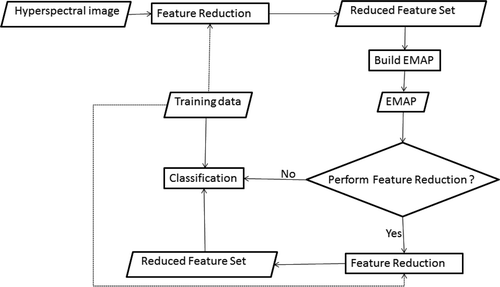
The general overview of the work flow for the classification of hyperspectral images using the EMAP is shown in Figure 1. Feature reduction is performed on the hyperspectral image and the resulting features are used to build the EMAP. The feature reduction can either be supervised or unsupervised. A further feature reduction operation applied to the EMAP can both reduce the effect of the Hughes phenomenon and the redundancy in the profiles for classification. The classification is usually performed using non-linear classifiers due to the fact that the resulting EMAP is characterised by highly non-linear class distributions.

Figure 1. The work flow of spectral-spatial classification with EMAP. The dotted lines indicate the possibility of switching between supervised and unsupervised feature reduction. An optional feature reduction step can be used to reduce the dimensionality of EMAP before classification.

In this work, two unsupervised (i.e. PCA and KPCA) and three supervised feature reduction methods (i.e. DAFE, DBFE and NWFE) are considered. In the case of unsupervised methods, PCA is a linear method while KPCA is a non-linear method. More details on these techniques can be found in Fukunaga (1990) and Schölkopf et al. (1998). The selection of the kernel parameters for KPCA is sometimes done by a supervised way using the training samples, but in this work a fixed value is used for the kernel parameter. It is calculated as two times the mean of all the pairwise distances of all the samples. For supervised methods, DAFE aims at identifying linear features that increase the separability between classes. On the other hand, DBFE uses the training samples to imply a decision boundary between the classes and uses this to extract the optimal features. NWFE can be seen as a method which combines the advantages of both DAFE and DBFE. NWFE exploits different weights for different samples focusing on samples close to the decision boundary. DAFE only produces k − 1 features for k classes and is less effective when the class means are similar, which is often the case with impervious classes. DBFE is computationally expensive as it depends on the training samples. Furthermore, the DBFE may give sub-optimal features for a small number of training samples when it may not be possible to get the best approximation of decision boundary. Therefore, NWFE might perform better in the case where there are a limited number of samples. We refer the reader to Landgrebe (2003) for a more complete presentation of these latter supervised feature extraction techniques.

The Random Forest™ (RF) (Breiman 2001) and support vector machines (SVM) (Schölkopf and Smola 2002) are used in this work for classifying the EMAP. While both methods are shown to be effective non-linear classifiers, SVM requires an exhaustive (computationally intensive) parameter tuning (e.g. model selection performed on a grid) for optimal results, whereas RF does not require any such tuning and is found to be more robust. The comparison of the theoretical aspects of these classifiers is out of scope of this article and is not presented here.

4. Experimental setup

4.1 Dataset description

The two standard datasets, namely AVIRIS Indian Pines dataset and the ROSIS University of Pavia dataset, which are frequently used in the literature, are used in this work.

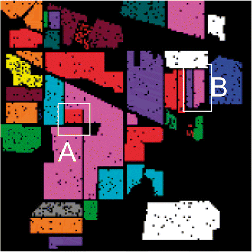
(1) Indian Pines dataset: The Indian Pines dataset is a standard dataset acquired in 1992 using the Airborne Visible Infrared Imaging Spectrometer (AVIRIS) sensor. It is an image with a spatial resolution of 20 m, consisting of 220 bands in the 400–2500 nm wavelength range. This dataset is one of the most widely used datasets in the literature for testing various methodologies corresponding to the hyperspectral data analysis. A false colour composite of the data is shown in Figure 2. Table 1 shows the ground truth classes and the number of available test pixels.

Figure 2. Indian Pine dataset. (a) False colour representation of the Indian Pines image, (b) test and (c) training sets.

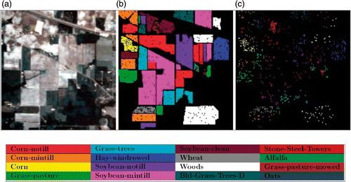
Table 1. Number of training and test pixels used for the Indian Pines image.

Class	Training	Test
Corn-notill	50	1384
Corn-mintill	50	784
Corn	50	184
Grass-pasture	50	447
Grass-trees	50	697
Hay-windrowed	50	439
Soybean-notill	50	918
Soybean-mintill	50	2418
Soybean-clean	50	564
Wheat	50	162
Woods	50	1244
Bld-grass-trees-D	50	330
Stone-steel-towers	50	45
Alfalfa	15	39
Grass-pasture-mowed	15	11
Oats	15	5

2) University of Pavia dataset: The image is a standard dataset acquired within the framework of the European Union HySens project using a ROSIS-3 instrument on the flight operated by the German Aerospace Center (DLR) over the University of Pavia in Pavia, Italy. It consists of 115 bands in the range of 0.43–0.86 µm at a spatial resolution of 1.3 m. Twelve noisy channels were removed leading finally to 103 bands. A false colour composite of the images is shown in Figure 3. Table 2 shows the ground reference classes and the number of available training and test pixels for every class.

Figure 3. Pavia University dataset. (a) False-colour representation of the University of Pavia image, (b) test and (c) training set.

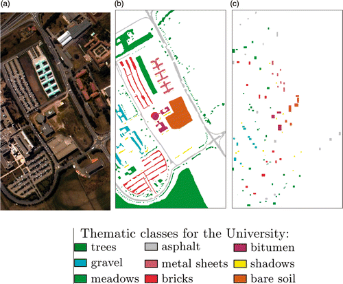
Table 2. Number of training and test pixels used for the Pavia image.

Class	Training	Test
Trees	524	2912
Asphalt	548	6304
Bitumen	375	981
Gravel	392	1815
Metal sheets	265	1113
Shadow	231	795
Bricks	514	3364
Meadows	540	18,146
Bare soil	532	4572

4.2 Setup

Several experiments are carried out to observe the effectiveness of EMAPs and various feature reduction methods. Furthermore, the effect of feature reduction of the EMAPs is also studied. While the APs can be built using a large number of attributes, only area and standard deviation attributes are considered in this work as they can be more easily calculated and are well-related to the object hierarchy in the images. Area is an increasing attribute (thus leading to have attribute opening and closing operators), whereas the standard deviation of the pixels values is non-increasing. The subtractive rule (Salembier and Wilkinson 2009) has been considered as filtering strategy when considering this latter attribute.

In all the cases but for NWFE, the features corresponding to the top few eigenvalues which account for 99% of the total sum of the eigenvalues were selected. For NWFE, 90% was chosen as it requires many more features to cover 99%. KPCA is done with 2000 samples selected uniformly over the entire image. The kernel parameter is chosen as twice the mean distance of all the sample pairs. Therefore, it needs to be noted that the number of features differs for each feature reduction method considered. The estimation of the covariance of the data, which especially for problems dealing with high-dimensional patterns can lead to singularity problems, is performed using the leave one out covariance estimate (Hoffbeck and Landgrebe 1996) for all the supervised feature reduction techniques.

The experiments are done with RF and SVM classifiers. The SVM classifier is tuned once the parameters of its model (e.g. the parameters defining the kernel) are defined. It is well known that the performances of an SVM strongly rely on the model selection procedure. In all the experiments with the SVM classifier, a radial basis function (RBF) was considered as kernel. An RF classifier is defined by setting the number of trees and the number of variables used in the classification process. Five-fold cross-validation is used to set the parameters of SVM. According to previous experiments, it was seen that the RF classifier is more robust than SVM to variations of the values of the model parameters. Thus, in all the experiments the number of trees was set to 200 and the cardinality of the subset of features considered for each split of the classification tree was equal to the square root of the total number of features (as suggested in Breiman 2001). The classification results are compared using the class-specific accuracies, overall accuracy (OA), average accuracy (AA) and κ coefficient.

The results of classification using the spectral information only are indicated using the names of the feature reduction methods as PCA, KPCA, DBFE, DAFE and NWFE. The classification results using the corresponding EMAPs are indicated with a prefix p (e.g. DAFE _p ). The additional experiments where a feature reduction is performed on the EMAP are denoted using the first two initials of the corresponding methods (e.g. NW-NW for NWFE feature reduction applied to the EMAP of NWFE features; KP-DB for the DBFE feature reduction applied to the EMAP of KPCA features).

5. Experimental results and discussion

5.1 Indian Pines data

As can be seen in Table 1, this dataset has a limited number of training samples for some classes. The classifications are done using the EMAP built with various features of reduction methods. Threshold values in the range of 2.5–10% with respect to the mean of the individual features with a step of 2.5% are chosen for the standard deviation attribute and thresholds of 200, 500 and 1000 are selected for the area attribute. The threshold values for standard deviation are adaptively chosen according to the automatic technique presented in Marpu et al. (2012), unlike previous works published in the literature, in which fixed values were considered. The thresholds of area are chosen based on both the resolution of the data and the fact that it is an agricultural area and the individual fields are slightly larger in size compared to urban areas.

Table 3. Accuracies (%) for classification of Indian Pines image. The best results in terms of accuracy are marked in bold.

Panel A: Results using RF with spectral information only
Cass	Spectral	PCA	KPCA	DAFE	DBFE	NWFE
Features	220	10	25	15	20	20
1	51.16	56.65	55.27	52.96	49.13	75.22
2	51.28	66.84	73.21	52.17	47.96	63.9
3	81.52	72.83	86.41	78.26	70.11	84.24
4	88.81	91.50	93.74	84.12	79.64	92.39
5	82.50	87.66	83.36	88.38	89.24	92.54
6	90.21	96.58	92.48	98.18	98.63	98.86
7	69.28	62.09	77.78	60.46	62.31	81.26
8	51.24	58.44	59.76	38.96	42.68	56.53
9	65.60	74.29	72.16	65.96	68.09	78.19
10	93.83	97.53	98.15	97.53	98.77	99.38
11	81.27	90.27	88.5	84.81	85.05	93.41
12	70.00	67.27	73.03	82.12	70.00	74.24
13	95.56	100	100	97.78	93.33	97.78
14	56.41	87.18	82.05	53.85	48.72	76.92
15	72.73	90.91	90.91	100	81.82	100
16	80.00	100	100	40.00	20.00	100
AA	73.83	81.25	82.93	73.47	69.09	85.30
OA	65.59	71.19	73.03	63.49	63.12	76.53
κ	61.33	67.46	69.63	59.00	58.50	73.50
Panel B: Results of RF with profiles
Class	PCA p	KPCA p	DAFE p	DBFE p	NWFE p	NW-NW	KP-NW
Features	130	325	195	260	260	30	30
1	82.23	89.88	77.75	77.46	91.04	88.44	80.20
2	95.15	97.70	85.71	83.93	98.21	94.01	93.37
3	96.74	96.74	91.30	86.41	97.83	90.22	95.65
4	94.18	94.41	93.96	92.17	93.96	93.74	94.41
5	98.71	98.42	97.42	97.99	99.71	96.99	98.57
6	99.54	99.54	99.77	100	100	99.54	98.63
7	89.87	86.71	75.27	88.13	88.67	82.03	78.21
8	91.27	93.92	72.42	82.09	93.22	89.62	91.11
9	92.38	95.74	79.96	85.28	95.21	92.73	90.25
10	99.38	99.38	98.77	99.38	99.38	99.38	99.38
11	99.44	99.76	98.63	94.94	99.52	90.51	93.41
12	97.27	98.48	98.18	90.00	98.79	95.76	99.09
13	100	100	100	100	100	100	100
14	94.87	92.31	97.44	97.44	97.44	94.87	97.44
15	100	100	100	100	100	100	100
16	100	100	100	80.00	100	100	100
AA	95.69	96.44	91.66	90.95	97.06	94.24	94.36
OA	92.83	94.76	84.33	87.22	95.06	91.03	90.36
κ	91.80	93.40	82.20	85.43	94.34	89.75	89.00
Panel C: Results using SVM with spectral information only
Class	Spect.	PCA	KPCA	DAFE	DBFE	NWFE
Features	220	10	25	15	20	20
1	53.47	62.21	66.04	47.76	50.29	66.55
2	58.16	65.31	75.64	43.88	47.58	53.57
3	78.80	84.78	83.15	75.54	75.54	78.80
4	85.68	89.04	94.85	87.47	84.34	89.93
5	80.20	90.96	90.82	84.51	86.08	90.96
6	94.99	93.39	94.76	98.18	96.58	98.18
7	78.43	65.69	79.85	58.50	62.64	72.88
8	59.51	55.67	64.52	43.88	47.68	46.86
9	61.52	68.26	77.48	64.18	67.55	79.26
10	95.68	98.15	98.77	99.38	99.38	99.38
11	90.27	93.49	90.03	84.41	85.21	84.73
12	54.24	62.42	72.42	82.12	78.18	75.15
13	97.78	95.56	97.78	93.33	93.33	95.56
14	51.28	76.92	92.31	43.59	64.10	74.36
15	81.82	81.82	90.91	72.73	90.91	81.82
16	100	100	100	20.00	40.00	60.00
AA	76.36	80.23	85.58	68.72	73.09	78.00
OA	69.70	71.55	77.31	62.71	64.90	69.79
κ	65.76	67.87	74.3	57.97	60.32	66.03
Panel D: Results using SVM with profiles
Class	PCA p	KPCA p	DAFE p	DBFE p	NWFE p	NW-NW	KP-NW
Features	130	325	195	260	260	30	30
1	72.47	79.41	58.09	66.91	79.62	90.24	84.03
2	87.37	92.73	58.67	76.28	79.34	98.85	98.21
3	91.85	96.20	83.70	84.78	83.15	97.28	98.91
4	91.28	93.96	93.29	92.62	93.29	95.52	97.54
5	98.42	98.42	86.51	94.84	95.55	99.56	98.85
6	98.63	98.63	94.76	98.41	99.32	99.54	99.32
7	79.96	87.36	67.97	75.16	78.32	86.27	89.11
8	83.83	87.84	56.00	65.47	65.55	94.58	93.71
9	84.22	86.35	69.68	81.21	88.83	93.61	87.41
10	99.38	99.38	96.91	99.38	99.38	99.38	99.38
11	94.86	95.90	87.46	89.71	92.36	92.76	98.63
12	94.24	96.36	95.15	91.52	95.15	99.09	99.09
13	100	100	82.22	97.78	97.78	100	100
14	92.31	94.87	30.77	79.49	79.49	94.87	97.44
15	100	90.91	18.18	63.64	100	100	100
16	100	100	20.00	60.00	100	100	100
AA	91.80	93.64	68.71	82.32	89.196	96.35	96.35
OA	86.53	90.20	70.69	78.39	81.853	94.17	93.75
κ	84.67	88.82	66.80	75.50	79.43	93.33	92.84

Table 4. Accuracies in percentage for classification of the University of Pavia image. The best results in terms of accuracy are marked in bold.

Panel A: Results using RF with spectral information only
Class	Spect.	PCA	KPCA	DAFE	DBFE	NWFE
Features	103	4	20	8	25	18
1	98.69	99.05	98.96	92.75	93.93	98.24
2	81.28	77.45	79.61	82.75	84.93	86.4
3	84.44	80.98	85.26	83.83	85.49	90
4	52.74	49.69	50.88	71.94	67.51	60.74
5	99.11	99.11	99.48	100	99.85	99.78
6	98.10	98.52	97.15	97.99	98.2	99.79
7	91.06	89.44	89.27	82.78	87.53	93.48
8	55.61	56.37	57.05	72.05	66.88	64.08
9	79.22	76.4	77.37	89.06	93.8	93.16
AA	82.25	80.78	81.67	85.91	86.46	87.3
OA	71.57	70.61	71.51	79.93	78.9	78.49
κ	65.07	63.82	64.89	74.63	73.62	73.26
Panel B: Results using RF with profiles
Class	PCA p	KPCA p	DAFE p	DBFE p	NWFE p	DB-DB	DA-DB	KP-DB
Features	68	340	136	425	306	26	30	30
1	99.15	99.90	92.36	96.93	99.44	94.97	98.82	99.08
2	94.86	96.54	95.86	97.60	96.83	96.54	95.62	96.57
3	99.70	99.84	100	99.32	99.77	100	99.92	99.84
4	67.56	94.33	88.32	81.41	66.46	74.51	74.41	76.13
5	99.63	99.77	99.85	99.85	99.70	100	100	99.70
6	99.79	99.89	96.30	99.89	100	98.52	99.26	96.93
7	99.02	99.80	99.51	98.47	99.45	99.37	98.39	99.67
8	96.48	94.04	98.08	96.72	97.72	98.53	80.54	87.39
9	73.28	64.44	88.06	90.87	61.10	97.31	89.99	78.76
AA	92.16	94.28	95.37	95.67	91.16	95.53	92.99	92.68
OA	92.76	92.37	95.87	95.83	92.19	96.81	88.16	90.13
κ	90.36	89.85	94.55	94.49	89.51	95.79	84.81	87.14
Panel C: Results using SVM with spectral information only
Class	Spect.	PCA	KPCA	DAFE	DBFE	NWFE
Features	103	4	20	8	25	18
1	97.98	97.68	98.56	86.88	94.75	90.21
2	84.35	70.25	79.49	79.16	81.77	82.23
3	91.88	85.56	89.32	83.76	86.47	87.37
4	71.37	55.93	63.41	66.84	71.37	71.13
5	99.33	98.44	99.48	99.78	99.63	99.78
6	97.99	94.4	94.93	99.16	98.2	98.84
7	92.69	86.34	89.84	80.74	84.95	89.35
8	70.44	58.05	69.7	67.83	66.79	64.1
9	93.64	72	85.54	87.87	91.85	94.43
AA	88.85	79.85	85.59	83.56	86.2	86.38
OA	81.44	69.68	78.68	76.56	78.19	77.48
κ	76.74	62.6	73.28	70.64	72.78	72
Panel D: Results using SVM with profiles
Class	PCA p	KPCA p	DAFE p	DBFE p	NWFE p	DB-DB	DA-DB	KP-DB
Features	68	340	136	425	306	26	30	30
1	98.73	99.64	97.09	94.97	96.93	95.43	98.53	96.96
2	92.34	94.11	93.15	92.84	92.14	95.88	94.98	95.27
3	99.70	99.24	99.92	98.05	97.07	100	99.92	99.77
4	61.03	92.28	79.99	68.84	82.71	90.94	76.46	90.13
5	99.48	99.62	99.33	99.93	99.93	100	100	99.77
6	89.23	99.15	96.62	96.09	97.25	98.41	98.31	99.36
7	99.16	99.40	97.12	94.84	97.28	99.18	98.78	98.26
8	96.14	89.70	98.36	89.38	82.13	98.65	91.93	88.20
9	92.36	78.16	99.44	98.83	97.77	99.96	97.30	87.73
AA	92.02	94.59	95.67	92.64	93.69	97.60	95.13	95.05
OA	93.89	91.52	96.62	91.64	89.27	97.89	93.98	91.80
κ	91.95	88.92	95.55	89.14	86.24	97.22	92.14	89.34

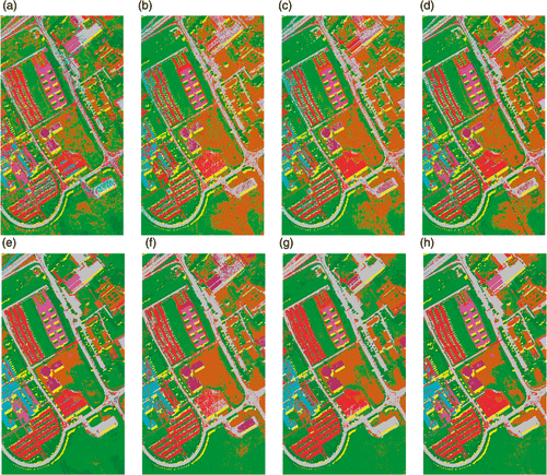
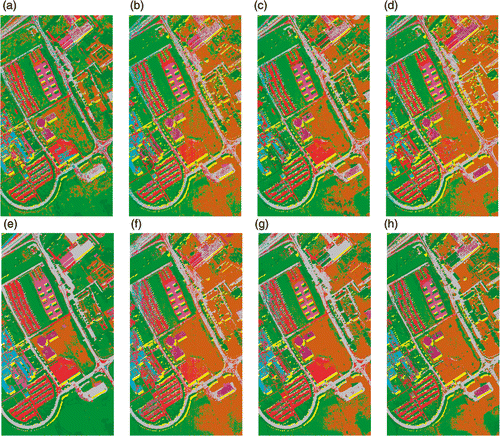
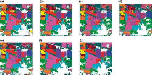
The results of the classification of the Indian Pines image are shown in Table 3 and the corresponding classification maps resulting from RF and SVM classifiers are shown in Figures 4 and 5, respectively, for classification using spectral information only and in Figures 6 and 7 for classification using EMAPs. The experiments are carried out with the mentioned feature reduction techniques.

Figure 4. Classification maps for Indian Pines data with RF classifier using (a) Original data (b) PCA, (c) KPCA, (d) DAFE, (e) DBFE and (f) NWFE.

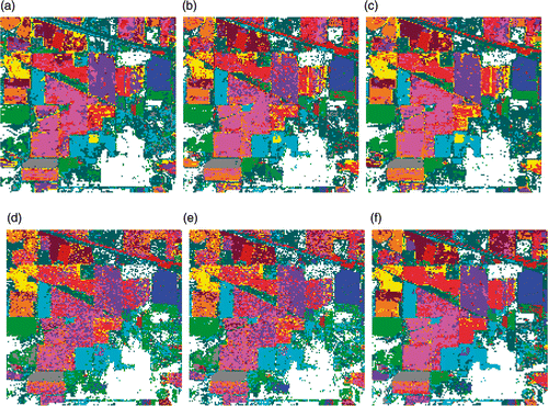
Figure 5. Classification maps for Indian Pines data with SVM classifier using (a) Original data (b) PCA, (c) KPCA, (d) DAFE, (e) DBFE and (f) NWFE.

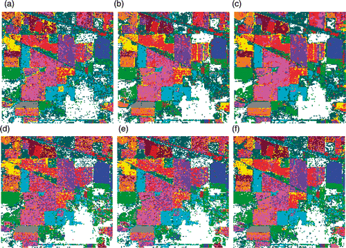
Figure 6. Classification maps for Indian Pines data with RF classifier using EMAPs of (a) PCA, (b) KPCA, (c) DAFE, (d) DBFE and (e) NWFE, and feature reduction applied on EMAP using (f) NW-NW and (g) KP-NW.

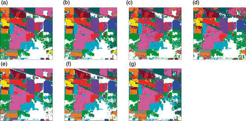
Figure 7. Classification maps of Indian Pines data with SVM classifier using EMAPs of (a) PCA, (b) KPCA, (c) DAFE, (d) DBFE and (e) NWFE, and feature reduction applied on EMAP using (f) NW-NW and (g) KP-NW.

It can be observed from the results that the RF consistently provides higher accuracies compared to SVM when directly using the EMAP, but SVM performs better in terms of accuracies when a feature reduction is applied to the EMAP. This shows the effectiveness of the RF classifier in dealing with the high-dimensionality space in input to the classifier. On the other hand, feature reduction of the EMAP degrades the accuracy of the RF classifier. This may depend on the fact that the RF classifier is based on a tree of weak classifiers, which can statistically take advantage from a large set of redundant features. On the contrary, the SVM classifier is expected to be more effective in designing the discriminant function when a subset of non-redundant features defines a highly non-linear problem.

The best results in terms of accuracies are obtained by using EMAPs built with NWFE and KPCA. NWFE with RF classifier provides the highest overall accuracy. SVM provides slightly lower, yet comparable, accuracies when a further feature reduction is applied to the EMAP. With the SVM, supervised feature reduction of the EMAP defined with both NWFE and KPCA using NWFE provides very similar performances in terms of accuracies. It is interesting to note that the classification of the EMAP of NWFE provides high accuracy, while the classification of EMAPS of DAFE and DBFE do not exhibit good accuracy. This shows that NWFE is more suitable for supervised feature reduction when a limited number of training samples are available.

Some interesting observations can be made while comparing the results when only spectral information derived from various feature reduction methods is used and the corresponding results when spatial information with EMAPs is used. The first observation is that significantly higher accuracies are achieved when profiles are used as was outlined in the literature. The second observation is that the results of classifying the EMAPs do not necessarily correlate with the performance of the classifiers when only spectral information is used. When the RF classifier is used, the accuracy of the result of classifying the KPCA features is much lower compared to the NWFE features, but the accuracies of the corresponding results using EMAPs are very similar. The obtained accuracies of SVM using NW-NW and KP-NW are similar, while the EMAP classification of KPCA produces higher accuracy in comparison to the EMAP classification of NWFE. At the same time, the results using DAFE and DBFE show that enough spectral information could not be captured in the feature reduction process to be able to discriminate the classes by exploiting the spatial information. While RF produces similar accuracies for DAFE and DBFE features and the corresponding EMAPs, the SVM produces higher accuracies for DBFE when compared to DAFE.

By visually comparing the classification maps, the results seem to be spatially more homogeneous when EMAP of KPCA is used, which is an indication that the spatial information is used effectively. However, a closer look at the ground truth shown in Figure 8 reveals that the unsupervised feature reduction carried out by PCA and KPCA could not correctly classify the object in the area denoted by A in Figure 8. Only the supervised feature reduction methods could discriminate that object from the local background. This is due to the fact that the object has similar spectrum as the background, and thus is difficult to separate using unsupervised methods. However, given the training samples, it is possible to extract better features to discriminate it from the background. None of the feature reduction methods provided features that could correctly classify the area denoted by B in Figure 8, even if EMAPs of PCA and KPCA performed slightly better than the others. A visual comparison of the classification maps points out that this area is highly non-homogenous and the selected training pixels probably do not fully represent the spectral variability of the class, thus resulting in a sub-optimal representation in the EMAP. Overall, on the one hand, it can be concluded that the supervised feature reduction is biased towards the training samples considered and their capability to properly represent the different classes of interest. On the other hand, the unsupervised methods could not effectively distinguish between similar spectra. The utilisation of spatial information too could not completely resolve the problem.

Figure 8. The ground reference data for the Indian Pines image. The segments shown in white boxes are found to be difficult to classify.

5.2 University of Pavia Data

As one can see in Table 3, a large number of training pixels are available for the experiments. The threshold values of 2.5–10% with respect to the mean of the individual features with a step of 2.5% are chosen for the definition of the criteria based on the standard deviation attribute (Marpu et al. 2012). Values of 100, 200, 500 and 1000 are selected as references for the attribute area. The threshold values considered for the area attribute are chosen according to the resolution of the data and, thus, the size of the objects present in the scene.

The results of the classification of the Pavia image are shown in Table 4, Figures 9–12. The experiments are carried out with the mentioned feature reduction methods and feature reduction on EMAPs was carried out using DA-DB, DB-DB and KP-DB.

Figure 9. Classification maps for University of Pavia data with RF classifier using (a) Original data (b) PCA, (c) KPCA, (d) DAFE, (e) DBFE and (f) NWFE.

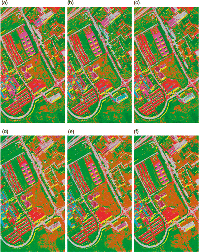
Figure 10. Classification maps for University of Pavia data with SVM classifier using (a) Original data (b) PCA, (c) KPCA, (d) DAFE, (e) DBFE and (f) NWFE.

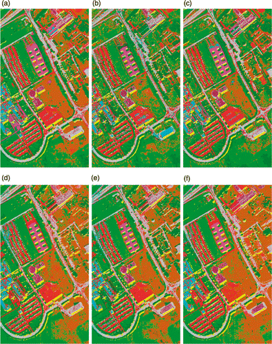
Figure 11. Classification results of University of Pavia data with RF classifier using EMAPS of (a) KPCA, (b) DBFE, (c) NWFE and feature reduction applied on EMAP using (d) DB-DB.

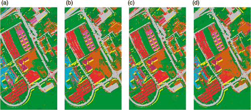
Figure 12. Classification maps of University of Pavia data with SVM classifier using EMAPS of (a) KPCA, (b) DBFE, (c) NWFE and feature reduction applied on EMAP using (d) DB-DB.

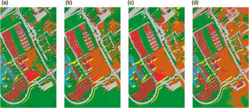
As expected, the classification based on EMAP and supervised feature reduction techniques performs well in this case due to the availability of sufficient training samples. The highest accuracy is obtained with DBFE feature reduction applied to the EMAP features computed on the DBFE components and using the SVM classifier. Conversely, when considering the RF classifier, the Gravel class was not correctly classified. Whereas, when the EMAP is used for classification, only the EMAP of KPCA could correctly classify the Gravel class. However, it could not effectively distinguish between Meadows and Bare Soil, which are the main contributors of the relatively low accuracy of the classification with the EMAP of KPCA. This can be easily understood as both these classes are characterised by high intra-class variability and have very similar spectra (i.e. low inter-class variability).

While using only the spectral information, NWFE, DAFE and DBFE all seem to produce similar accuracies, but when the corresponding EMAPs are used for classification, the accuracies are quite different indicating that the classification with EMAPs do not necessarily follow the trend of classification with spectral information only. It depends on how well the class objects are discriminated from the background region using different feature reduction methods.

Surprisingly, the DAFE _p and DBFE _p both outperform NWFE _p in terms of classification accuracies except for the Trees class. Accordingly, in the case of a sufficient set of available training samples, it can be stated that both DAFE and DBFE obtain more discriminant features compared to those obtained by NWFE. This effect of considering a reduced number of training samples can be verified by the results reported in Tables 5 and 6. It is also interesting to note that SVM, in this scenario, provides similar or better accuracies compared to those obtained by RF (unlike as the results of Indian Pines dataset). This shows that the number of samples and the dimensionality of the data have a clear influence on the relative accuracies on the classification results of both the RF and SVM classifiers.

Table 5. Accuracies in percentage for classification of Pavia image with 30 training pixels per class. The best results in terms of accuracy are marked in bold.

Panel A: Results using RF with spectral information only
Class	DBFE	DAFE	NWFE	KPCA
Features	10	8	15	20
1	89.13	90.6	96.54	96.08
2	76.4	74	74.44	72.06
3	88.35	87.82	91.05	82.41
4	67.08	70.94	54.07	50.21
5	100	99.85	99.33	98.88
6	99.68	99.89	99.89	99.26
7	82.07	73.82	83.98	79.85
8	70.84	68.92	57.73	56.5
9	82.12	76.26	79.38	62.58
AA	83.96	82.46	81.82	77.54
OA	77.22	74.89	71	67.25
κ	71.24	68.34	64.13	59.39
Panel B: Results using RF with profiles
Class	DBFEp	DAFEp	NWFEp	KPCAp
Features	150	120	225	300
1	87.63	87.14	98.49	98.79
2	89.12	91.87	94.87	95.52
3	98.64	86.09	99.62	97.66
4	63.17	72.41	69.84	97.42
5	99.85	100	99.92	99.55
6	99.36	99.68	100	99.89
7	87.01	71.89	98.42	98.42
8	87.49	81.58	89.82	87.82
9	90.47	86.95	80.85	62.97
AA	89.20	86.40	92.42	93.12
OA	87.87	84.04	90.77	89.20
κ	84.20	79.39	87.90	85.81
Panel C: Results using SVM with spectral information only
Class	DBFE	DAFE	NWFE	KPCA
Features	10	8	15	20
1	91.12	87.53	89.85	94.81
2	71.27	66.01	63.04	72.39
3	88.87	85.56	89.02	80.60
4	70.84	73.27	64.13	58.50
5	99.70	99.78	99.41	99.03
6	99.79	99.16	99.89	99.47
7	78.68	64.67	72.35	73.28
8	60.13	56.19	54.63	54.08
9	89.60	88.15	88.84	63.77
AA	83.33	80.04	80.13	77.33
OA	72.68	68.52	67.95	66.09
κ	66.32	61.40	60.81	58.15
Panel D: Results using SVM with profiles
Class	DBFEp	DAFEp	NWFEp	KPCAp
Features	150	120	225	300
1	89.72	94.13	96.89	97.94
2	87.66	54.68	81.87	91.11
3	82.26	66.99	95.78	98.72
4	65.46	65.27	68.74	82.61
5	87.06	65.72	99.40	98.95
6	98.52	91.55	98.83	99.57
7	58.01	47.45	82.69	97.71
8	67.83	45.70	63.34	86.54
9	82.76	75.88	91.58	84.37
AA	79.92	67.49	86.57	93.06
OA	75.00	57.53	76.80	89.64
κ	68.43	49.06	71.20	86.56

Table 6. Accuracies in percentage for classification of Pavia image with 100 training pixels per class. The best results in terms of accuracy are marked in bold.

Panel A: Results using RF with spectral information only
Class	DBFE	DAFE	NWFE	KPCA
Features	20	8	18	20
1	91.29	87.70	97.32	97.72
2	80.46	79.37	79.55	70.22
3	84.74	76.69	90.15	87.29
4	63.70	67.17	67.27	58.60
5	100	100	99.93	99.63
6	99.16	99.68	99.89	99.47
7	84.03	76.43	89.27	82.54
8	68.91	63.54	61.26	58.38
9	93.44	88.41	92.15	73.73
AA	85.08	82.11	86.31	80.84
OA	78.37	74.29	75.99	70.03
κ	72.86	67.93	70.33	63.00
Panel B: Results using RF with profiles
Class	DBFEp	DAFEp	NWFEp	KPCAp
Features	300	120	270	300
1	96.21	83.61	99.09	99.37
2	97.01	95.12	95.60	95.06
3	99.84	98.57	100	99.47
4	85.08	69.12	68.79	93.56
5	100	100	99.93	99.77
6	99.89	97.25	100	100
7	98.96	96.60	98.64	99.61
8	98.13	97.24	97.39	91.10
9	81.84	97.89	63.89	61.06
AA	95.22	92.82	91.48	93.2292
OA	95.49	94.71	92.22	90.3661
κ	93.98	92.98	89.56	87.24
Panel C: Results using SVM with spectral information only
Class	DBFE	DAFE	NWFE	KPCA
Features	20	8	18	20
1	92.00	85.77	84.14	97.88
2	76.88	69.54	71.29	68.81
3	85.19	77.37	84.14	88.72
4	67.56	66.51	65.27	69.32
5	99.93	100	99.85	99.70
6	99.16	99.16	98.94	96.73
7	81.29	78.27	81.50	83.24
8	66.19	59.81	57.48	67.56
9	93.24	88.35	94.73	69.78
AA	84.60	80.53	81.93	82.42
OA	76.62	71.13	71.44	73.94
κ	70.88	64.31	64.97	67.30
Panel D: Results using SVM with profiles
Class	DBFEp	DAFEp	NWFEp	KPCAp
Features	300	120	270	300
1	93.14	86.49	98.76	98.98
2	90.71	79.34	84.92	90.95
3	98.57	92.41	94.06	99.24
4	67.98	67.22	76.70	89.23
5	99.85	100	99.63	99.92
6	99.78	94.93	98.42	99.36
7	89.62	81.04	88.24	99.21
8	76.56	71.01	70.45	91.78
9	98.72	97.73	95.63	87.03
AA	90.55	85.57	89.64	95.08
OA	85.18	79.33	81.79	92.78
κ	81.18	74.02	77.16	90.56

In order to evaluate the geometrical precision of the classification maps, nine objects are considered as shown in Figure 13, which shows a snapshot of a recent very high resolution image from Google maps.1 It can be noted that all the selected objects have not changed from the time of the acquisition of the ROSIS data used in the experiments. Among all the considered objects, only the objects C and I contain pixels that are part of the original reference set of labelled samples used for the accuracy assessment. The spectra of some of the objects like A, D, E, F, G and H probably cannot be related to the classes of interest identified in the given reference data. The presence of such objects in the scene means that we can investigate the bias of the supervised feature reduction towards the classes of interest. The following observations can be made with respect to the classification results of various experiments for the considered objects.

Figure 13. A snapshot of University of Pavia region from Google Maps (accessed 02 November 2011). A big part of the image remains unchanged from the date of acquisition of the ROSIS image. The boxes delineates specific areas considered in the discussion to visually compare the geometric stability of the classification results. Imagery ©2011 DigitalGlobe, GeoEye.

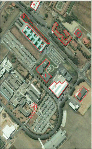
Object A is a building with metallic roof and hence should have a relatively similar spectrum compared to Object C, which forms a part of the training and reference data. However, an observation of the classification maps indicates that only EMAP of KPCA with RF classifier could correctly detect this object. It was misclassified as tree class using SVM. None of the other results show any consistent classification and the shape of the object is also not well preserved.

Object B is made up of bushes, thus, it should be spectrally similar to the tree and meadows classes in the reference data. This confusion is clearly seen in the results. While considering EMAPs based on KPCA and DBFE classify it as trees, the other classifiers associate this object as Meadows. Only the results with KPCA seem to maintain the geometric characteristics of this object.

Object C is a student dormitory with metal sheets on the roof. The bright area just above the object C, which is a parking area, should be ideally classified as the bricks class in the reference data. However, the spectrum of the pixels belonging to this object seems to be a bit different to the spectra of the pixels belonging to the bricks class in reference data. The area of the parking lots merges in the classification maps with the roof of the adjacent building when KPCA is used. However, this issue does not occur when supervised feature reduction is used. The geometric characteristics of the object are preserved only when considering EMAP of DBFE and RF.

Object D is another student dormitory where the roof is covered with clay tiles. This class is not represented in the reference data and there is no stability of this object in any classification results. However, according to some classification maps, the spectra of the pixels belonging to the roof are more similar to the Bare soil class. However, the shapes of the objects seem to remain stable in most of the classification maps.

Object E and G have similar spectra, but again they are not related to any classes in the reference data. They are classified as bitumen in all the cases, and hence are merged with road objects. Although they are not correctly represented in the thematic maps, their external boundaries are precisely extracted.

Object F is a building with metallic roof, but its spectral signature seems to be different to those of the objects used in reference data. Only by using KPCA it was possible to correctly extract the shape of the object.

Object H is a pathway made of cement blocks and is not represented in the reference data. Among all the feature extraction techniques, only when considering KPCA it is possible to represent precisely the shape of this object in the classification maps.

According to the observations reported above, it is clear that there is a significant difference between the results when considering different feature extraction methods. The profiles built with unsupervised feature reduction seem to maintain the geometric features of objects with spectra different to that of their background, but the capability of distinguishing between structures with slightly similar spectra becomes low as is evident when looking at object C. This effect is in accordance with the conclusions drawn on the results of the Indian Pines dataset. The EMAPs built with supervised feature reduction has a high bias towards the classes of interest and the training data. In this latter case, it is also observed that the geometric shapes of the objects which are not represented in the reference data are not preserved well.

5.3 Experiments using reduced training samples

Two additional experiments were done using the University of Pavia dataset with a reduced number of training samples, in order to confirm the observed behaviour in the above experiments on the effect of the number of samples on the different supervised feature reduction algorithms and their EMAPs. The first experiment was done with 30 training pixels per class sampled randomly using a uniform random number generator from the training samples shown in Figure 3. The second experiment was done with 100 samples per class sampled in the same way. The EMAPs were constructed with 5%, 7.5% and 10% of the feature mean as thresholds for the standard deviation attribute and sizes of 100, 200, 500 and 1000 are selected as references for the area attribute.

The classification accuracies obtained when using 30 samples per class are shown in Table 5, and the corresponding classification maps are shown in Figures 14 and 15 using RF and SVM classifiers, respectively. The best accuracies in this case were obtained using EMAPS of NWFE and KPCA, as was observed in the case of Indian Pines data. The classification map obtained with EMAP of KPCA is composed of more homogeneous regions as there is less influence of noise, which would be present in supervised feature reduction due to inadequate number of samples. Again the major problem with KPCA is the confusion between Meadows and Bare soil classes.

Figure 14. Classification maps of University of Pavia data using 30 training samples per class with RF classifier using (a) KPCA, (b) DAFE, (c) DBFE, (d) NWFE, (e) KPCA _{p ,} (f) DAFE _{p ,} (g) DBFE _p and (h) NWFE _p .

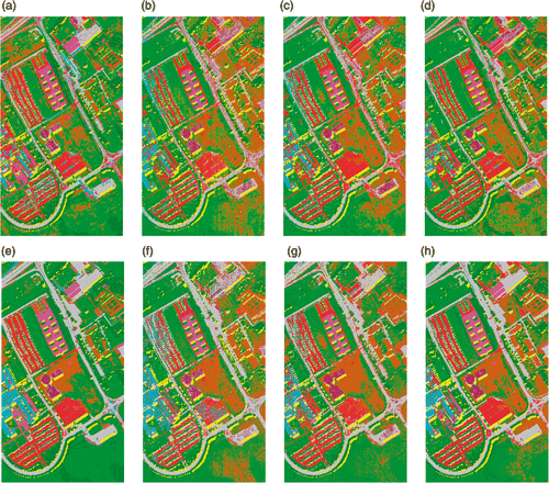
Figure 15. Classification maps of University of Pavia data using 30 training samples per class with SVM classifier (a) KPCA, (b) DAFE, (c) DBFE (d) NWFE, (e) KPCA _{p ,} (f) DAFE _{p ,} (g) DBFE _p and (h) NWFE _p .

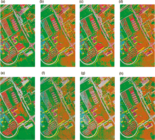
The classification accuracies and maps using 100 training samples per class are shown in Table 6 (Panel A) and in Figure 16 for RF and in Table 6 (Panel B) and Figure 17 for SVM. The results show that EMAP of DBFE now has the highest accuracy, indicating that sufficient training samples are available to obtain more optimal features which can discriminate the class objects from the background. This is similar to what is observed in the experiments with full training data. EMAP of KPCA also performs well, barring the Meadows class. Again the results of KPCA are spatially more homogeneous compared to those generated by the supervised methods.

Figure 16. Classification maps of University of Pavia data using 100 training samples per class with RF classifier using (a) KPCA, (b) DAFE, (c) DBFE, (d) NWFE, (e) KPCA _{p ,} (f) DAFE _{p ,} (g) DBFE _p and (h) NWFE _p.

Figure 17. Classification maps of University of Pavia data using 100 training samples per class with SVM classifier using (a) KPCA, (b) DAFE, (c) DBFE, (d) NWFE, (e) KPCA _{p ,} (f) DAFE _{p ,} (g) DBFE _p and (h) NWFE _p .

6. Conclusions

The aim of this article is to explore the suitability of various feature reduction algorithms to create base images for EAPs when used in spectral-spatial classification. Five supervised and unsupervised feature reduction methods were considered as two classifiers. Experiments were conducted using two standard datasets, namely AVIRIS Indian Pines and ROSIS University of Pavia. Further experiments were carried out using reduced training data in the case of Pavia data to see the effect of the number of training samples. The following conclusions can be made.

1.	The accuracies of spectral-spatial classification with APs of features from various feature reduction methods do not necessarily follow the same trend as using the spectral information only.
2.	The EMAP based on KPCA produces more accurate classification, but there can be problems when the classes are difficult to separate. Moreover, neighbouring objects with similar spectra can be merged together in the classification maps, as observed in the experiments with both the datasets. KPCA preserves the shapes of the objects which are not represented by any training sample.
3.	In terms of the classification accuracies obtained in the experiments, NWFE was the best supervised feature reduction algorithm when the size of the training data was small, whereas DBFE provided the best results when sufficient training data were available.
4.	The shapes of the objects that are not represented by the training data may not be preserved when using supervised feature reduction methods even while using the profiles.
5.	The dimensionality of the input data has an influence on the accuracy provided by the different classifiers considered in this study. RF seems to be more suitable to work in the high-dimensional feature space which contains redundant features in comparison to the SVM classifier.

In general, EMAP based on KPCA was found to be more consistent even if it produces slightly inferior accuracies compared to the supervised feature reduction methods. However, it is difficult to determine which supervised feature reduction can be better suited as it depends on the training samples. So, it might be interesting to find a way to fuse the results of classifying EMAPs from different feature reduction methods. As future developments of this work, we aim at extending the experimental analysis considering other hyperspectral datasets with high spatial resolution and a wide range of feature reduction algorithms. Moreover, motivated by the promising results obtained on the considered datasets, we plan to test the proposed approach on large-scale images in order to assess computational issues and to provide insights for an optimisation and complete automation of the classification process.

Notes

1. http://maps.google.com.

References

- Benediktsson , JA , Palmason , JA and Sveinsson , JR . 2005 . Classification of hyperspectral data from urban areas based on extended morphological profiles . IEEE Transactions on Geoscience and Remote Sensing , 43 ( 3 ) : 480 – 491 .
- Benediktsson , JA , Pesaresi , M and Arnason , K . 2003 . Classification and feature extraction for remote sensing images from urban areas based on morphological transformations . IEEE Transactions on Geoscience and Remote Sensing , 41 ( 9 ) : 1940 – 1949 .
- Breen , EJ and Jones , R . 1996 . Attribute openings, thinnings, and granulometries . Computer Vision and Image Understanding , 64 ( 3 ) : 377 – 389 .
- Breiman , L . 2001 . Random forests . Machine Learning , 45 ( 1 ) : 5 – 32 .
- Castaings , T . 2010 . On the influence of feature reduction for the classification of hyperspectral images based on the extended morphological profile . International Journal of Remote Sensing , 31 ( 22 ) : 5921 – 5939 .
- Dalla Mura , M , Benediktsson , JA and Bruzzone , L . 2010a. Classification of hyperspectral images with extended attribute profiles and feature extraction techniques. In: International geoscience and remote sensing symposium (IGARSS), Honolulu, HI, 76–79
- Dalla Mura , M . et al., 2011a. The evolution of the morphological profile: from panchromatic to hyperspectral images. In: S. Prasad, L. Mann Bruce and J. Chanussot, eds. Optical remote sensing – advances in signal processing and exploitation techniques. Springer Verlag, 123–146
- Dalla Mura , M . 2010b . Extended profiles with morphological attribute filters for the analysis of hyperspectral data . International Journal of Remote Sensing , 31 ( 22 ) : 5975 – 5991 .
- Dalla Mura , M . 2010c . Morphological attribute profiles for the analysis of very high resolution images . IEEE Transactions on Geoscience and Remote Sensing , 48 ( 10 ) : 3747 – 3762 .
- Dalla Mura , M . 2011b . Classification of hyperspectral images by using extended morphological attribute profiles and independent component analysis . IEEE Geoscience and Remote Sensing Letters , : 541 – 545 .
- Datcu , M , Seidel , K and Walessa , M . 1998 . Spatial information retrieval from remote-sensing images – part I: information theoretical perspective . IEEE Transactions on Geoscience and Remote Sensing , 36 ( 5 ) : 1431 – 1445 .
- Daya Sagar , BS and Serra , J . 2010 . Spatial information retrieval, analysis, reasoning and modelling . International Journal of Remote Sensing , 31 ( 22 ) : 5747 – 5750, 2010 .
- Fauvel , M . Chanussot, J., and Benediktsson, J. A., 2009. Kernel principal component analysis for the classification of hyperspectral remote sensing data over urban areas. EURASIP Journal on Advances in Signal Processing, 2009, 14
- Fukunaga , K . 1990 . Introduction to statistical pattern recognition , 2nd , London , , UK : Academic Press .
- Hoffbeck , J and Landgrebe , DA . 1996 . Covariance matrix estimation and classification with limited training data . IEEE Transactions on Pattern Analysis and Machine Intelligence , 18 ( 7 ) : 763 – 767 .
- Landgrebe , DA . 2003 . Signal theory methods in multispectral remote sensing , London : Wiley-Inter Science .
- Licciardi , G . et al., 2012. Linear versus non-linear PCA for the classification of hyperspectral data based on the extended morphological profiles. IEEE Geoscience and Remote Sensing Letters, 9 (3), 447–451
- Maragos , P and Ziff , R . 1990 . Threshold superposition in morphological image analysis systems . IEEE Transactions on Pattern Analysis and Machine Intelligence , 12 ( 5 ) : 498 – 504 .
- Marpu , PR . et al., 2012. Automatic generation of standard deviation attribute profiles for spectral-spatial classification of remote sensing data. IEEE Geoscience and Remote Sensing Letters, accepted for publication
- Ouzounis G.K., and Soille, P., 2009. Differential area profiles. In: 20th International conference on pattern recognition, 23–26 August 2009, Istanbul, Turkey, 4085–4089
- Peeters , S . et al., 2011. Classification using Extended Morphological Attribute Profiles based on different feature extraction techniques. In: IEEE International Geoscience and Remote Sensing Symposium (IGARSS), 24–29 July 2011, Vancouver, Canada, 4453–4456
- Pesaresi , M and Benediktsson , JA . 2001 . A new approach for the morphological segmentation of high-resolution satellite imagery . IEEE Transactions on Geoscience and Remote Sensing , 39 ( 2 ) : 309 – 320 .
- Salembier , P , Oliveras , A and Garrido , L . 1998 . Anti-extensive connected operators for image and sequence processing . IEEE Transactions on Image Processing , 7 ( 4 ) : 555 – 570 .
- Salembier , P and Wilkinson , MHF . 2009 . Connected operators . IEEE Signal Processing Magazine , 26 ( 6 ) : 136 – 157 .
- Schölkopf B., and Smola A.J., 2002. Learning with kernels: support vector machines, regularization, optimization, and beyond. Cambridge, MA, USA: MIT Press
- Schölkopf , B , Smola , AJ and Müller , K-R . 1998 . Nonlinear component analysis as a kernel eigenvalue problem . Neural Computation , 10 : 1299 – 1319 .
- Soille , P . 2003 . Morphological image analysis. Principles and applications , 2nd , Berlin , , Germany : Springer Verlag .
- Soille , P and Pesaresi , M . 2002 . Advances in mathematical morphology applied to geosciences and remote sensing . IEEE Transactions on Geoscience and Remote Sensing , 40 : 2042 – 2055 .
- Wilkinson , MHF . 2008 . Concurrent computation of attribute filters on shared memory parallel machines . IEEE Transactions on Pattern Analysis and Machine Intelligence , 30 ( 10 ) : 1800 – 1813 .
- Wilkinson M.H.F., Soille P., and Ouzounis, G.K., 2010. Concurrent computation of differential morphological profiles for remote sensing. In: Workshop on Applications of Digital Geometry and Mathematical Morphology, 26–29 September, Istanbul, Turkey
- Wilkinson , MH . 2011 . “ Concurrent computation of differential morphological profiles on giga-pixel images ” . In Mathematical morphology and its applications to image and signal processing , Edited by: Soille , P , Pesaresi , M and Ouzounis , G . 331 – 342 . Berlin, Heidelberg : Springer .