A multi-domain decomposition strategy for the lattice Boltzmann method for steady-state flows

ABSTRACT

The lattice Boltzmann method (LBM) is a potent numerical technique based on kinetic theory. It can effectively simulate the steady-state and unsteady-state flow problems. A multi-domain decomposition strategy is developed for the LBM in order to accelerate the rate of convergence in different domains by the relative error in the different regions of the steady-state flow. In addition, the proposed method can effectively reduce the amount of calculations required and improve numerical stability. Numerical experiments involving both two- and three-dimensional steady-state flows demonstrate drastically improved computational efficiency and superior numerical stability over the popular lattice Bathnagar-Gross-Krook (BGK) model. Moreover, for unsteady-state flow problems, the presented method can also be used to obtain the flow phenomenon of some unsteady-state flows by choosing the suitable parameter.

KEYWORDS:

• Lattice Boltzmann method
• multi-domain decomposition strategy
• Bathnagar–Gross–Krook model
• steady-state flows

1. Introduction

In the past two decades, the lattice Boltzmann method (LBM) has been developed into a viable numerical tool for computational fluid dynamics (CFD) and beyond. The LBM is based on kinetic theory, but is a truly mesoscopic method. Hydrodynamic variables are computed at the nodes as moments of the discrete distribution function. The LBM was originally designed for uniform structured grids. The popularity of this method in flow problems is the simplicity of formulation compared with solving the Navier–Stokes (NS) equations, and it has several advantages over other conventional CFD methods, especially in dealing with complex boundaries, incorporating microscopic interactions, and parallelization of the algorithm (Aidun & Clausen, 2010; Chen & Doolen, 1998; Succi, 2001). In recent years, many researchers have studied the multi-block strategy and multi-grid strategy based on the LBM by using a non-uniform structure grid. Multi-scale lattice Boltzmann equation (LBE) schemes were proposed and the boundary-fitting formulation was discussed (Filippova & Hänel, 1998a, 1998b), while multi-scale LBE schemes were tested and validated for moderate Reynolds number flows around cylinders and blades (Filippova & Hänel, 1998a, 1998b, 2000; Mazzocco, Arrighetti, Bella, Spagnoli, & Succi, 2000).

The multi-block method can improve the accuracy and computational efficiency of the LBE schemes for viscous flow computations (Yu, Mei, & Shyy, 2002). Mavriplis (2006) investigates the efficient solution strategies for the steady-state LBE by using a non-linear multi-grid approach which can converge to a steady state rapidly. By taking advantage of the merits of both coarse and fine meshes, the LBM with double meshes accelerates the convergence rate and improves the efficiency of computation (Wang, Luo, Cheng, & Liu, 2003). Another multi-block and multi-grid method can be found in Guo and Zheng (2009). Currently, the interface condition of the multi-block method or the multi-grid method is derived to ensure the mass conservation and stress continuity between neighboring blocks. The main aim of these multi-scale methods is to improve the efficiency of the LBM. Recently, Touil, Ricot, and Lévêque (2014) carried out multi-resolution simulations of turbulent flows using the LBM (D3Q19 model), which can accurately simulate the complex turbulent flows. With these rules used in these multi-scale methods, the evolution of collision and streaming is computed at the same time-step.

For the final flow state in the steady-state flows, the final exact state will not change with time. In addition, the rate of convergence in the different regions of the steady-state flow can be considered. By combining a multi-domain decomposition strategy with the traditional LBM in uniform structure grids, a multi-domain decomposition strategy will be constructed for the LBM for steady-state flows in order to improve the computational efficiency. For the different steady-state flows, different multi-domain decomposition strategies are used in order to improve the numerical stability and computational efficiency of the LBM. Moreover, the classical LBM combined with turbulence modeling (Filippova et al., 2001) or large eddy simulation (LES; Hou, Sterling, Chen, & Doolen, 1996) can be used to solve incompressible flow. The steady-state incompressible flow can also be solved by the presented method using turbulence modeling or LES.

The rest of the paper is organized as follows. In Section 2, the multi-domain decomposition strategy for the LBM is described in detail and its corresponding algorithms is presented, then the numerical results are presented in Section 3, and Section 4 concludes the paper.

2. The multi-domain decomposition strategy for the lattice Boltzmann method (LBM)

In this section, the lattice BGK model, including D2Q9 and D3Q19, is introduced. Combined with the multi-domain strategy, the multi-domain decomposition strategy for the LBM is presented in detail.

2.1. The lattice BGK model

The lattice BGK model is described by the change rate of a discrete velocity distribution function (Qian, D'Humières, & Lallemand, 1992): (1) where is a set of discrete populations representing the density of particles at position and time t moving in the direction identified by the discrete speed , is a set of equilibrium discrete populations, is the time interval, and τ is the relaxation time which characterizes a typical collision process. In the two- and three-dimensional cases we consider the D2Q9 and D3Q19 velocity models, respectively. The D2Q9 and D3Q19 velocity models are as follows: (2)

Here, the lattice speed is , where and are the grid size and the time-step size, respectively. The equilibrium distribution for D2Q9 and D3Q19 velocity model is in the form of (3) where is the macro velocity and the corresponding weighting coefficients are (4)

With the discrete velocity space, the density and momentum fluxes can be computed as (5)

The speed of sound in these models is and the pressure is given by the equation of state of an ideal gas,

For the uniform structure grid computation, the specific identification of the time level for the post-collision state is not important since the completion of the computational step in the LBM occurs at the end of the streaming step (Yu et al., 2002). Due to its extreme simplicity, the lattice BGK equation has become the most popular LBM. Next we will construct the multi-domain decomposition strategy for the LBM in the uniform structure grid.

2.2. The multi-domain decomposition strategy for the LBM

In this subsection, we describe a novel multi-domain decomposition strategy for use with the LBM, which is different from the multi-block and multi-grid variants (Filippova et al., 2001; Wang et al., 2003; Yu et al., 2002). We also use the uniform structure grid with dependence on the flow problem. In order to accelerate the convergence rate of the lattice BGK model, we divide the multi-domain by the different flows. The multi-domain version of the LBM might result in improved numerical stability and a better convergence rate.

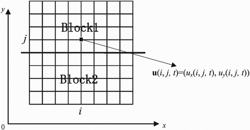
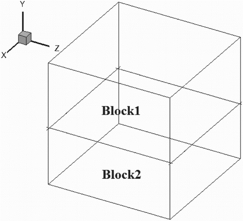
In order to illustrate the basic idea of the new method, we will give a two-domain strategy in two dimensions (Figure 1), which is described below in detail. For the convenience of presentation, we consider the lattice BGK model (D2Q9) as an example.

Figure 1. A two-domain decomposition strategy, Block1 and Block2.

Firstly, we define the relative error in each iteration step as follows: (6)

In Figure 1, the uniform structure grid is divided into two domains (Block1 and Block2). In the calculation, each domain needs to compute the relative error using Equation (6(6) ). The relative error of Block1 and Block2 is defined as Error1 and Error2, respectively.

Depending on the steady-state flow problems, such as lid-driven cavity flow, the second block (Block2) will produce lower left and lower right vortex, so it is possible that Error2 will be bigger than Error1 in the same iteration steps. Then we define two specific values for the relation between the error in Block1 and Block2: (7)

Furthermore, we need to give the open parameter ϵ a non-negative number; this can be used to adjust the computational efficiency of the presented method. Next, we present some evolution rules between each block of the multi-domain version of the LBM in the uniform structure grid.

Case 1. If then the evolution of Block1 is suspended (paused) but Block2 continues the evolution of collision and streaming by Equation (1(1) ) until the condition of is reached.

Case 2. If then the evolution of Block2 is suspended (paused) but Block1 continues the evolution of collision and streaming by Equation (1(1) ) until the condition of is reached.

Case 3. If and then Block1 and Block2 (the whole flow field) are calculated using Equation (1(1) ).

In Case 1 and Case 2, we need to define some rules in the information exchange on the interface between the neighboring blocks. Let us use Case 1 as an example. Because the relative error of Block1 (Error1) is smaller than that of Block2 (Error2), the evolution of streaming in Block2 on the interface between Block1 and Block2 can use the interface information from Block1. So the information in Block2 is constantly updated, while the updating of Block1's information is temporarily terminated. If the condition is reached then the information exchange between the two blocks resumes. For Case 2, we can also adopt the same treatment similar to Case 1. Furthermore, Case 3 will ensure that the fluid information is consistent throughout the whole flow field.

The main purpose of the evolution rule is that Block1 and Block2 have a synchronized convergence rate, which results in an accelerated convergence rate and improved computational efficiency and numerical stability, etc. On the other hand, the multi-domain decomposition strategy for the LBM can be suitable for parallel computing, because the Message Passing Interface (MPI) process of each block can reduce the communication cost. Furthermore, the proposed method can be used to solve higher Reynolds values in steady-state incompressible flows used the same scale grids, such as a lid-driven cavity flow at by (see the next section).

Next, we will consider the value of the parameter ϵ. The choice of value for ϵ is key to the efficiency of the convergence rate. According to the above, but is not a fixed value, thus for different flow problems, a different value can be chosen to suit the situation. In the next section, we will give some ranges for the value of ϵ using numerical simulations.

The evolution rules are based on two blocks in the above. We can also use these rules to solve for multi-block setups, as the multi-block scenario can be considered as a number of sets of two blocks. However, the evolution rules become more complex when the number of blocks increases, and the frequency of the information exchange between these blocks increases. In the next section, we present the four-domain strategy for solving the lid-driven cavity flow and the three-domain strategy for solving the flow around a circular cylinder. In addition, we can also use the presented method to solve a three-dimensional flow.

2.3. The algorithm of the multi-domain decomposition strategy for the LBM

Based on the description in the previous subsection, we will give the corresponding algorithm in this subsection. We also use the two-domain strategy (see Figure 1) as an example to present the algorithm below.

Here, N, the positive integer in Step 3 fin Algorithm 1, is used to ensure that the whole flow field has the initial information, namely and . Generally, N can be given by the length or width of the flow field.

In order to illustrate the presented method, we will consider the unsteady-state flow problem. While the proposed method is produced from the steady-state flows, it also can be used to solve some unsteady-state flows. After some changes are made to the numerical simulation, the flow phenomenon can be obtained – but there are some specific time offsets required because the computation of each block in Case 1 and Case 2 is not at the same time-step, while the computation of all blocks in Case 3 is at the same time-step. So the flow of the specific time may not exact. In unsteady-state flows, after some iteration steps the computation of Case 3 continues but the computation of Case 1 and Case 2 is terminated, so the flow phenomenon will be exact after enough iteration steps. Some examples of this are presented in the next section.

3. Numerical results

In this section, we will verify the numerical stability and accuracy of the multi-domain decomposition strategy for the LBM in uniform structure grids by simulating the two- and three-dimensional lid-driven cavity flow, the flow around a circular cylinder and the flow around a sphere. For the boundary conditions, the non-equilibrium extrapolation scheme proposed by Guo, Zheng, and Shi (2002) is used. For the curved boundary, we will adopt the YMS scheme (Yu, Mei, & Shyy, 2003). For the two-dimensional lid-driven cavity flow we present the two-domain and four-domain strategies, while the three-domain strategy is used for the flow around a circular cylinder. We also provide the two examples of three-dimensional, lid-driven cavity flows and the flow around a sphere by using the two-domain decomposition strategy. In this section, the convergence condition is the relative error in the all flow field domain (see Equation (6(6) )) which is less than in two- and three-dimensional lid-driven cavity flows.

3.1. Two-dimensional lid-driven cavity flow

The two-dimensional lid-driven cavity flow has been extensively used as a benchmark solution to test the accuracy of a numerical method. To assess the results of the multi-domain decomposition strategy for the LBM, the benchmark solutions of several schemes are used for comparative purposes (Ghia, Ghia, & Shin, 1982; He, Wang, & Li, 2009).

In a two-dimensional lid-driven cavity flow, the upper boundary of the square cavity moves horizontally to the right at a constant speed, while the other three boundaries remain stationary. In the numerical simulation, the flow field initial density , the lid driven speed U=0.1. The Reynolds numbers Re is set to 400, 1000, 5000, and 10000, respectively.

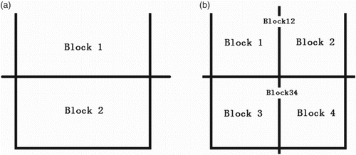
Figure 2 shows the partitioning strategy for two blocks and four blocks. In this example, . First we consider the two-block scenario. The computations are carried out using three cases: (I) a single block with a uniform structure grid () using the lattice BGK model, (II) two blocks with a uniform structure grid (), and (III) two blocks with a uniform structure grid () using the multi-domain decomposition strategy for the LBM.

Figure 2. The multi-domain decomposition strategy for (a) two blocks; (b) four blocks.

In Table 1, we provide the iteration steps for each block using the multi-domain decomposition strategy for the LBM where for Cases (I) and (II).

Table 1. The iteration steps for each block (two-domain decomposition strategy) for a two-dimensional lid-driven cavity flow.

Re		Block1	Block2	Block12	Steps
400	0	–	–	–	58,216
	2	0	15,333	47,675	63,008
1000	0	–	–	–	205,075
	2	0	20,500	114,915	135,415
5000	0	–	–	–	>1,000,000
	2	581	36,013	261,633	298,227
10,000	0	–	–	–	>1,000,000
	2	287	85,986	850,871	937,144

Note: The column headings Block1, Block2, and Block12 represent the iteration steps of Block1, Block2 and the whole flow field (Block1 + Block2), respectively. Steps is the total iteration number, and when , this indicates that the traditional lattice BGK model is adopted.

At , the number of iterations of the presented method seems slightly larger than that of the traditional LBM. However, the amount of calculations required in Block2 is only half in the whole flow field in the presented method. The number of iteration steps is only 55,342, and the number of iterations are 125,165 for Re = 1000, then 279,930 for Re = 5000, and 894,008 for Re = 10,000.

At and 10,000, the number of iteration steps of the traditional LBM reaches more than 1,000,000, but the proposed method has a better convergence rate. With the Reynolds number increased, the multi-domain decomposition strategy has a better convergence rate than the traditional LBM in Table 1. Furthermore, may not be the optimal value, but it has obtained better computational efficiency for the multi-domain decomposition strategy, so is a good choice that is also used in the next subsection.

Figures 3, 4, and 5 show the streamlines of the two-dimensional lid-driven cavity flow at , , and , respectively. From Figures 3 to 5, using the multi-domain decomposition strategy for the LBM, three vortices (the primary vortex, the lower-left vortex, and the lower-right vortex) are computed at , 1000, and 5000, while two vortices (the left-upper vortex and the second-lower-right vortex) are computed at . Figure 6 shows the streamlines of the two-dimensional lid-driven cavity flow at . The five vortices are also computed. The locations of the vortices, as well as the results from Ghia et al. (1982) (using the Finite Differencing Method (FDM) NS solver) and He et al. (2009) (using the D2Q9 LBM), are listed in Table 2. It can be seen that the numerical results are in excellent agreement with the experimental data. The results also prove the validity of the multi-domain decomposition strategy for the LBM.

Figure 3. Streamlines in the two-dimensional cavity flow at for: (a) Case (I); (b) Case (II); (c) Case (III).

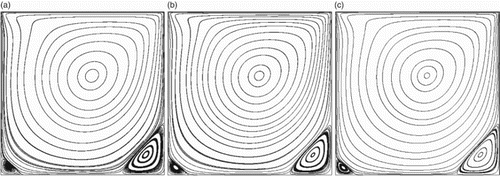
Figure 4. Streamlines in the two-dimensional cavity flow at for: (a) Case (I); (b) Case (II); (c) Case (III).

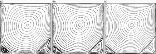
Figure 5. Streamlines in the two-dimensional cavity flow at for: (a) Case (I); (b) Case (II); (c) Case (III).

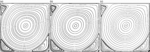
Figure 6. Streamlines in the two-dimensional cavity flow at for: (a) Case (I); (b) Case (III).

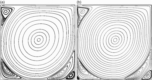
Table 2. The central locations of vortices for the lid-driven cavity flow for , and .

		Primary Vortex		Lower-left Vortex		Lower-right Vortex
Re		x	y	x	y	x	y
400	a	0.5547	0.6055	0.0508	0.0469	0.8906	0.1250
	b	0.5668	0.6069	0.0471	0.0482	0.8857	0.1231
	c	0.5573	0.6074	0.0482	0.0462	0.8854	0.1228
	d	0.5580	0.6084	0.0476	0.0453	0.8850	0.1237
1000	a	0.5313	0.5625	0.0859	0.0781	0.8594	0.1094
	b	0.5336	0.5675	0.0820	0.0731	0.8644	0.1128
	c	0.5335	0.5674	0.0815	0.0753	0.8648	0.1129
	d	0.5320	0.5654	0.0817	0.0741	0.8650	0.1131
5000	a	0.5117	0.5352	0.0703	0.1367	0.8086	0.0742
	b	0.5158	0.5458	0.0742	0.1337	0.80554	0.0745
	c	0.5161	0.5346	0.0744	0.1333	0.8091	0.0747
	d	0.5170	0.5372	0.0738	0.1365	0.8120	0.0733
10000	a	0.5117	0.5333	0.0586	0.1641	0.7656	0.0586
	b	–	–	–	–	–	–
	c	0.5123	0.5304	0.0603	0.1585	0.7783	0.0614
	d	0.5123	0.5289	0.0587	0.1628	0.7862	0.0611
Re		Upper-left Vortex		Second-lower-right Vortex
Re		x	y	x	y
5000	a	0.0625	0.9102	0.9805	0.0195
	b	0.0638	0.9084	0.9836	0.0160
	c	0.0630	0.9082	0.9842	0.0155
	d	0.0616	0.9088	0.9822	0.0163
10000	a	0.0703	0.9141	0.9336	0.0625
	b	–	–	–	–
	c	0.0698	0.9117	0.9420	0.0557
	d	0.0695	0.9115	0.9412	0.0604

Note: a = Ghia et al. (1982) (with FDM NS solver); b = LBGK model (He et al., 2009); c = the multi-domain decomposition strategy for the LBM (257×257); d = the multi-domain decomposition strategy for the LBM ().

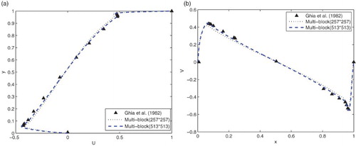
The velocity components u and v along the vertical and horizontal lines through the geometric center are shown in Figures 7, 8, 9, and 10 for Re = 400, 1000, 5000, and 10,000, respectively. According to Figures 7(b) to 10(b), the velocity u is accurate in the interface between Block1 and Block2. In Figure 10, the results using the grid are obviously better than the results using the grids. From Tables 1 and 2 and Figures 6 and 10, it can be seen that the multi-domain decomposition strategy for the LBM improves numerical stability and resolves the inability of the traditional lattice BGK method to calculate the higher Reynolds numbers for steady-state flows. Figures 7(b) to 10(b) show that the interface data of the two blocks is in agreement with the reference data (Ghia et al., 1982). These results of two-dimensional lid-driven cavity flow demonstrate the validity of the multi-domain decomposition strategy for the LBM.

Figure 7. Comparison of the profiles of the u-velocity through the geometric center in the present results and those of Ghia et al. (1982) at along: (a) the vertical line; (b) the horizontal line.

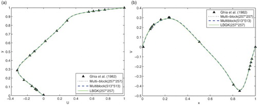
Figure 8. Comparison of the profiles of the u-velocity through the geometric center in the present results and those of Ghia et al. (1982) at Re = 1000 along: (a) the vertical line; (b) the horizontal line.

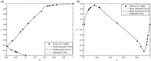
Figure 9. Comparison of the profiles of the u-velocity through the geometric center in the present results and those of Ghia et al. (1982) at Re = 5000 along: (a) the vertical line; (b) the horizontal line.

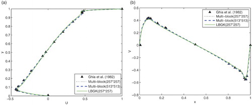
Figure 10. Comparison of the profiles of the u-velocity through the geometric center in the present results and those of Ghia et al. (1982) at Re = 10,000 along: (a) the vertical line; (b) the horizontal line.

Next, we will consider the case of four blocks (Figure 2(b)). Firstly, we introduce the four-blocks algorithm. In Figure 2(b), Block1 and Block2 are labelled Block12, while Block3 and Block4 are labelled Block34. Thus, Block12 and Block34 can be solved in a similar way to two-domain strategy (Figure 2(a)) using Algorithm 1. Secondly, Block1 and Block2 is the two-blocks case in Block12. Block3 and Block4 is also the two-blocks case in Block34. So we adopt the nested structure (two blocks) to solve the four-block two-dimensional lid-driven cavity flow. Before numerical simulation, we define some variables as follows: (8) where Error1, Error2, Error3, Error4, Error12, and Error34 are the relative error (see Equation (6(6) )) for Block1, Block2, Block3, Block4, Block12, and Block34, respectively. Based on the results of Table 1, we only consider and 10,000. The value of ϵ is , and .

In Table 3, we give the iteration steps for each block (four-domain strategy) for solving the two-dimensional lid-driven cavity flow at and 10,000. Compared with Table 1, the numbers of iteration steps in Table 3 are smaller; thus the result of the four-domain strategy shows a better convergence rate and improved numerical stability. As the Reynolds number increases, the convergence rate continues to improve.

Table 3. The iteration steps of each block (four-domain decomposition strategy) in a two-dimensional lid-driven cavity flow.

Re	Block1	Block2	Block3	Block4	Block12	Block34	Block1234	Steps
5000	0	0	470	198	519	27,577	232,024	260,788
10,000	2262	8870	3549	13,032	5613	62,043	712,016	807,385

Table 4. The central locations of vortices for the lid-driven cavity flow for and 10,000.

		Primary Vortex		Lower-left Vortex		Lower-right Vortex
Re		x	y	x	y	x	y
5000	a	0.5117	0.5352	0.0703	0.1367	0.8086	0.0742
	b	0.5169	0.5354	0.0734	0.1352	0.8107	0.0746
10000	a	0.5117	0.5333	0.0586	0.1641	0.7656	0.0586
	b	0.5122	0.5301	0.0603	0.1591	0.7809	0.0616
Re		Upper-left Vortex		Second-lower-right Vortex
		x	y	x	y
5000	a	0.0625	0.9102	0.9805	0.0195
	b	0.0624	0.9083	0.9850	0.0147
10000	a	0.0703	0.9141	0.9336	0.0625
	b	0.0698	0.9117	0.9427	0.0548

Note: a = Ghia et al. (1982) (with FDM NS solver); b = the multi-domain decomposition strategy.

In Table 4, by the four-domain decomposition strategy for the LBM, five vortices (the primary, lower-left, lower-right, left-upper, and second-lower-right vortices) are also computed at and . The locations of the vortices, as well as the results from Ghia et al. (1982) (with FDM NS solver), are given. When compared with Table 2, the locations of the vortices for the four-block strategy are in agreement with the results for the two-domain decomposition strategy, further proving the validity of the presented method.

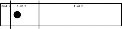
3.2. The flow around a circular cylinder

Although the flow in the square cavity is complex, the geometry is nevertheless simple because only flat boundaries are involved. To demonstrate the capability of the present multi-domain decomposition strategy for the LBM, we apply the method to two-dimensional flow around a circular cylinder. The cylinder is set into a channel with a uniform velocity at the inlet (Figure 11). The computation domain is and , where D is the diameter of the cylinder (for the boundary conditions, see Guo, Shi, & Wang, 2000). The Reynolds number , υ is the kinematic viscosity. Firstly, we use the three-domain decomposition strategy (Figure 11).

Figure 11. The multi-domain decomposition strategy in the flow around a circular cylinder (three blocks).

According to Sections 2 and 3.1, the numerical simulation is based on the two-domain strategy (see Algorithm 1). By combining Block2 and Block3, the three-block problem can become a two-block problem (Block1 and Block23) and thus the algorithm can also adopt the nested structure. Numerical simulations were carried out for a steady-state flow with small Reynolds numbers (, 20, and 40 where ϵ = 2, 2.1, and 2.1, respectively) based on a grid (Table 5). Figures 12, 13, and 14 show the streamlines of the steady-state flow around a circular cylinder at , 20, and 40, respectively. Table 5 provides the iteration steps of each block, and represents the use of the traditional lattice BGK method. The number of iteration steps using the proposed method is smaller than that of the traditional LBM at , 20, and 40, and the number of calculations needed is also smaller. Hence, the numerical results show that the multi-domain decomposition strategy for the LBM can improve the convergence rate and computational efficiency, as well as further proving its validity.

Figure 12. Streamlines of the steady-state flow around a circular cylinder at .

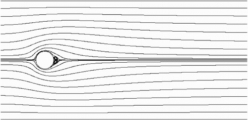
Figure 13. Streamlines of the steady-state flow around a circular cylinder at .

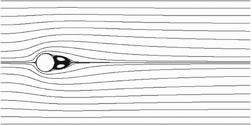
Figure 14. Streamlines of the steady-state flow around a circular cylinder at .

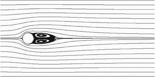
Table 5. The iteration steps for each block (three-domain decomposition strategy) in the flow around a circular cylinder.

Re		Block1	Block2	Block3	Block23	Block123	Steps
10	0	–	–	–	–	–	6455
	2	327	4	94	430	5445	6300
20	0	–	–	–	–	–	11,535
	2.1	432	152	76	296	7764	8720
40	0	–	–	–	–	–	19,900
	2.1	471	1211	2757	839	13,284	18,562

When in the flow around a circular cylinder, a Von Karman Vortex Street is a repeating pattern of swirling vortices caused by the unsteady separation of the flow of a fluid around blunt bodies. In this example, the convergence condition should set the number of iteration steps because the relative error will oscillate within a range. We set the number of iteration steps to 20,000 and the two-domain decomposition strategy is used. Block1 is and , and Block2 is and . The number of iteration steps for each block are given in Table 6, and the distribution of the computation of Block1 and Block2 can be seen in Figure 15, which shows that the computation of Block1 takes places during the first 6000 steps and the computation of Block2 takes place during steps 8000 to 15,000. After 15,000 steps, Block1 and Block2 are computing at the same time-step. Therefore, the results of the flow in 20,000 steps can be seen in Figure 16, in which the Von Karman Vortex Street is obtained and thus the flow phenomenon of the cylinder is computed by the presented method.

Figure 15. The computational distribution of each block at . Note: Blue represents the steps during which Block1 is computed, and green represents the steps during which Block2 is computed, while all flow fields are being computed in the remaining steps.

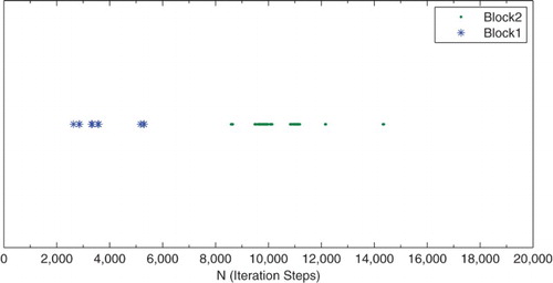
Figure 16. A Von Karman Vortex Street and streamlines of the flow around a circular cylinder at .

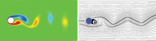
Table 6. The iterations of each block (two-domain decomposition strategy) in the flow around a circular cylinder.

Re		Block1	Block2	Block12	Steps
100	2	66	447	19,487	20,000

3.3. Three-dimensional lid-driven cavity flow

The validity of the multi-domain decomposition strategy for the LBM was proven for a two-dimensional steady-state flow in Sections 3.1 and 3.2. To demonstrate the capability of the presented method with a three-dimensional steady-state flow, we apply the presented method to a three-dimensional lid-driven cavity flow. The two-domain decomposition strategy is shown in Figure 17. The three-dimensional relative error is defined by (9)

Figure 17. The two-domain decomposition strategy for a three-dimensional lid-driven cavity flow.

In the numerical simulation, the lid-driven velocity , and the grid used is . Table 7 presents the iteration steps of each block for the three-dimensional lid-driven cavity flow. Similarly, Block12 represents the number of iteration steps for the whole flow field (Block1 and Block2), and represents the traditional LBM. In the numerical simulation . From Table 7, it can be seen that the presented two-domain version of the LBM has a better convergence rate.

Table 7. The iterations of each block for the three-dimensional lid-driven cavity flow.

Re		Block1	Block2	Block12	Steps
1000	0	–	–	–	30,100
	2	0	6423	21,545	27,968

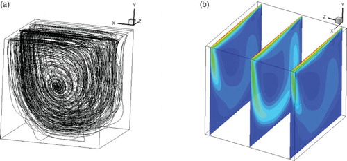
Figure 18 shows the three-dimensional streamlines of the cavity flow for and the velocity in the z-plane. The results of the three-dimensional lid-driven cavity flow also prove the validity of the multi-domain decomposition strategy for the LBM. Therefore, the presented method can also be used to improve the convergence rate and computational efficiency for three-dimensional steady-state flows.

Figure 18. (a) The streamlines and (b) the velocity for the three-dimensional lid-driven cavity flow at .

3.4. The flow around a three-dimensional sphere

To demonstrate the capability of the present multi-domain decomposition strategy for the LBM, we apply the method to three-dimensional flow around a sphere. The sphere is set into a channel with a uniform velocity at the inlet (Figure 19). The uniform grid is , the center coordinate of the sphere is , its diameter is 10, and the Reynolds number . We use the two-domain decomposition strategy (Figure 19) where Block1 and Block2 are of equal size and .

Figure 19. The two-domain decomposition strategy in the flow around a sphere.

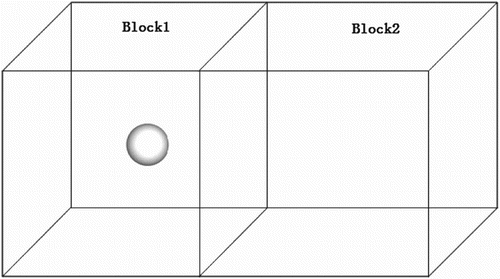
Table 8 presents the number of iteration steps for each block in the three-dimensional flow around a sphere, while Block12 represents the number of iteration steps for the whole flow field (Block1 and Block2) and represents the traditional LBM. From Table 8, it can be seen that the number of iteration steps for the presented method is smaller than that of the traditional LBM; thus, the proposed multi-domain version of the LBM has a better convergence rate for the three-dimensional steady-state flow around a sphere.

Table 8. The iterations of each block in the flow around a sphere.

Re		Block1	Block2	Block12	Step
100	0	–	–	–	11,746
	2	1249	906	9477	11,631

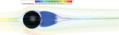
Figure 20 shows the three-dimensional streamlines of the flow around a sphere at . The color of the streamlines represents the magnitude of the velocity. The results of the flow around a sphere also prove the validity of the multi-domain decomposition strategy for the LBM. Therefore, the presented method can be used to improve the convergence rate and computational efficiency for three-dimensional steady-state flows.

Figure 20. The streamlines of the flow around a sphere .

In this numerical simulation, the sphere can be replaced with another object of arbitrary shape. According to the above results, the value of ϵ will usually be set to 2 for the different flows, and if the convergence rate is slow then a value near to 2.0 can be chosen.

In summary, two blocks and three blocks are widely used in the numerical simulations. The presented method is also suitable for strategies for other divisions, and the location of the division can be arbitrarily chosen as it only affects the convergence rate in steady-state flows – thus, any location is possible for ease of use before considering the convergence rate.

4. Conclusion

By combining a multi-domain decomposition strategy with the traditional lattice BGK method in a uniform structure grid, a multi-domain decomposition strategy was proposed for the LBM for solving steady-state flows. The main aim of this method was to accelerate the convergence rate of each block by the relative error and improve the numerical stability. The proposed method was used for two- and three-dimensional lid-driven cavity flows, the flow around a circular cylinder, and the flow around a sphere, and the numerical results demonstrate its validity. The proposed method has a lower number of iteration steps and a better convergence rate with higher Reynolds numbers in steady-state flows. Furthermore, the numerical examples also show drastically improved efficiency in comparison to the widely-used lattice BGK method. The value of ϵ can be used to adjust the convergence rate, but is generally set to 2 for the different flows. In addition, the presented method can be applied to solving other complex three-dimensional problems.

Funding

This work was supported by the National Natural Science Foundation of China [grant number 91330116] and the Doctoral Fund of the Ministry of Education of China [grant number 20133108110014].

References

• Aidun C. K., & Clausen J. R. (2010). Lattice-Boltzmann method for complex flows. Annual Review of Fluid Mechanics, 42, 439–472.
   Google Scholar
• Chen S., & Doolen G. D. (1998). Lattice Boltzmann method for fluid flows. Annual Review of Fluid Mechanics, 30, 329–364.
   Google Scholar
• Filippova O., & Hänel D. (1998a). Boundary-fitting and local grid refinement for lattice-BGK models. International Journal of Modern Physics C, 9, 1271–1279.
   Google Scholar
• Filippova O., & Hänel D. (1998b). Grid refinement for lattice-BGK models. Journal of Computational Physics, 147, 219–228.
   Google Scholar
• Filippova O., & Hänel D. (2000). Acceleration of lattice BGK schemes with grid refinement. Journal of Computational Physics, 165, 407–427.
   Google Scholar
• Filippova O., Succi S., Mazzocco F., Arrighetti C., Bella G., & Hänel D. (2001). Multiscale lattice Boltzmann schemes with turbulence modeling. Journal of Computational Physics, 170, 812–829.
   Google Scholar
• Ghia U., Ghia K. N., & Shin C. T. (1982). High-Re solutions for incompressible flow using the Navier-Stokes equations and a multigrid method. Journal of Computational Physics, 48, 387–411.
   Google Scholar
• Guo Z. L., Shi B. C., & Wang N. C. (2000). Lattice BGK model for incompressible Navier-Stokes equation. Journal of Computational Physics, 165, 288–306.
   Google Scholar
• Guo Z. L., & Zheng C. G. (2009). Theory and applications of Lattice Boltzmann method. Beijing: Science Press.
   Google Scholar
• Guo Z. L., Zheng C. G., & Shi B. C. (2002). Non-equilibrium extrapolation method for velocity and pressure boundary conditions in the lattice Boltzmann method. Chinese Physics, 11, 366–374.
   Google Scholar
• He Y. L., Wang Y., & Li Q. (2009). Lattice Boltzmann method: Theory and applications. Beijing: Science Press.
   Google Scholar
• Hou S., Sterling J., Chen S., & Doolen G. D. (1996). A lattice Boltzmann subgrid model for high Reynolds number flow fields. Fields Institution Communications, 6, 151–166.
   Google Scholar
• Mavriplis D. J. (2006). Multigrid solution of the steady-state lattice Boltzmann equation. Computers & Fluids, 35, 793–804.
   Google Scholar
• Mazzocco F., Arrighetti C., Bella G., Spagnoli L., & Succi S. (2000). Multiscale lattice Boltzmann schemes: A preliminary application to axial turbomachine flow simulations. International Journal of Modern Physics C, 11, 233–245.
   Google Scholar
• Qian Y. H., D'Humières D., & Lallemand P. (1992). Lattice BGK models for Navier-Stokes equation. Europhysics Letters (EPLP), 17, 479–484.
   Google Scholar
• Succi S. (2001). Lattice Boltzmann equation for fluid dynamics and beyond. Oxford: Clarendon Press.
   Google Scholar
• Touil H., Ricot D., & Lévêque E. (2014). Direct and large-eddy simulation of turbulent flows on composite multi-resolution grids by the lattice Boltzmann method. Journal of Computational Physics, 256, 220–233.
   Google Scholar
• Wang X. Y., Luo L. S., Cheng Y. G., & Liu D. Y. (2003). Lattice Boltzmann method with double meshes. Journal of Hydrodynamics, Ser. B, 15, 90–96.
   Google Scholar
• Yu D. Z., Mei R. W., & Shyy W. (2002). A multi-block lattice Boltzmann method for viscous fluid flows. International Journal for Numerical Methods in Fluids, 39, 99–120.
   Google Scholar
• Yu D. Z., Mei R. W., & Shyy W. (2003, January). A unified boundary treatment in lattice Boltzmann method. Paper presented at the 41st Aerospace Sciences Meeting and Exhibit, Reno, Nevada.
   Google Scholar

Disclosure statement

No potential conflict of interest was reported by the authors.