Flow field analysis of a pentagonal-shaped bridge deck by unsteady RANS

ABSTRACT

Long-span cable-stayed bridges are susceptible to dynamic wind effects due to their inherent flexibility. The fluid flow around the bridge deck should be well understood for the efficient design of an aerodynamically stable long-span bridge system. In this work, the aerodynamic features of a pentagonal-shaped bridge deck are explored numerically. The analytical results are compared with past experimental work to assess the capability of two-dimensional unsteady RANS simulation for predicting the aerodynamic features of this type of deck. The influence of the bottom plate slope on aerodynamic response and flow features was investigated. By varying the Reynolds number (2 × 10⁴ to 20 × 10⁴) the aerodynamic behavior at high wind speeds is clarified.

KEYWORDS:

• flow field
• pentagonal bridge deck
• separation interference method
• aerodynamic behavior
• unsteady RANS
• Reynolds number

1. Introduction

Cable-stayed bridges are one of the most popular and widely-used bridge configurations adopted by engineers for medium- to long-span bridges. Cable-stayed bridges are now being used to connect bodies of land that are much further apart as the deck can withstand much higher compressive loads due to increases in material strength and allowing for an increased bridge span length. However, as the span length of a bridge increases, it becomes more aerodynamically vulnerable due to its inherent flexibility. The bridge deck should be shaped to reduce aerodynamic loading and susceptibility to aero-elastic phenomenon such as vortex shedding and flutter instability. Usually, the slope of the bridge deck bottom plate is adjusted and fairings or flaps are attached to the basic bridge deck section to control the flow and improve aerodynamic stability. However, the addition of these extra devices increases the construction and maintenance costs.

Kubo and his associates (Kubo et al., 2007; Noda et al., 2009; Yoshida, Kubo, Tsuji, Kimura, & Kato, 2006) proposed an aerodynamically stable deck shape for cable-stayed bridges as shown in Figure 1. For this section no additional devices are required to increase the stability of the deck. The bottom deck flow is controlled by the bottom plate slope (θ), whilst the top deck flow is controlled by positioning the curb on the top deck; this technique is known as the separation interference method (SIM; Kubo et al., 2008; Yoshida et al., 2006). A number of long-span bridge decks have already been shaped based on these concepts, including the Takeshima Ohashi bridge, the Shintenmom bridge, the Oshima bridge, the Kesennuma bridge and the Ikara Ohashi bridge, in order to improve the aerodynamic performance of the deck. One of the advantages of this type of shape is that it exhibits negative lift values at high wind speeds – therefore, at high wind speeds the cable tension increases and the total stiffness of the bridge system enhances. Kubo et al. (2007) also showed the influence of the θ on flutter and vortex-shedding behavior using wind-tunnel experiments. They found that a θ of 12° has the lowest aerodynamic loading (specially, the drag is the lowest) and high flutter wind-speed. Then, Noda et al. (2009) and Noda (2010) clarified the cause of negative lift value from surface pressure distribution and particle image velocimetry (PIV) measurement for a pentagonal-shaped bridge deck with a θ of 14°. Their findings showed that it was the separated shear layer at the leading-edge bottom toe that generates suction and increases the negative lift value.

Figure 1. Schematic view of the aerodynamically stable bridge deck section.

From the PIV experiments of Noda et al. (2009), some of the flow mechanisms were identified. However, there is more to understand about the aerodynamics of this type of section. Noda et al. (2009) showed the role of the leading-edge bottom-deck separation on static lift force at a particular Reynolds number (R_e). However, there are a number of other flow features, such as top-deck leading-edge separation and bottom-deck trailing separation, the behavior and role of which in terms of aerodynamic response is not yet clear. Further, Kubo et al. (2007) showed that all the static aerodynamic coefficients exhibit very high sensitivity when the θ is altered at flutter wind-speed. All of these flow features will have a role in controlling the static and dynamic aerodynamic response of the bridge deck. It is important to know the role of these aerodynamic flow features on aerodynamic response and how those flow features behave when the shape of the deck is altered by changing the θ. Further, the R_e effect is also required to be clarified as the bridges are required to operate over a wide range of R_e. It is worth knowing how the increase in R_e affects the aerodynamic response and the flow field around the bridge deck. However, it is quite challenging to reveal the complete effect of varying the R_e. An interesting approach would be to find correlations of important flow features and the static response as the R_e gradually increases. Information regarding the influence of deck shapes and R_e on the flow field can be used to physically explain the quantitative response obtained from the wind-tunnel experiments of the pentagonal-shaped bridge deck. Moreover, this can also be applied to designing similar type of decks.

To improve the understanding of the response of the bridge deck, detailed visualization and analysis of flow field around the deck section is required. However, conventional wind-tunnel experiments demand very complicated instrumentation to capture the flow field and are expensive to use to conduct a large number of tests. Further, the quality of the obtained flow field deteriorates at high wind speeds (Blocken, 2014). An alternative approach is computational fluid dynamics (CFD), which is low cost and provides flow quantities at every location of the domain. Furthermore, no detailed numerical investigation has been carried out for this type of pentagonal-shaped bridge deck to reconfirm the experimental results and further understanding the flow mechanism. A number of researchers (Bruno & Mancini, 2002; Huang & Liao, 2011; Sarwar & Ishihara, 2010; Sarwar et al., 2008; Watanabe & Fumoto, 2008) have already shown the strength and efficiency of CFD in bridge aerodynamics. Unsteady Reynolds-averaged Navier-Stokes (RANS) and large eddy simulation (LES) are two very common and popular CFD approaches. LES has better accuracy, yet it is not a practical choice due to its huge computational load, especially for a large number of simulations. On the other hand, unsteady RANS has moderate accuracy with a high computational efficiency. A number of researchers have successfully applied unsteady RANS simulation to bridge aerodynamics and obtained useful results (Brusiani et al., 2013; Mannini, Soda, Voß, & Schewe, 2010; Nieto et al., 2010; Šarkić et al., 2012; Shirai & Ueda, 2003). Thus, we decided to conduct unsteady RANS simulations for this research.

The objective of the present study is to employ CFD to explore the aerodynamic features of a pentagonal-shaped bridge deck. First, the capability of unsteady RANS was confirmed by predicting the aerodynamic response of the pentagonal-shaped deck where massive flow separation occurs. To pursue this, simulations were carried out for a pentagonal-shaped deck and compared with previous experimental work (Kubo et al., 2007; Noda, 2010). Then, simulations were carried out for the pentagonal-shaped deck using various values of θ to explore the aerodynamics. Essentially, the mean and root mean square (RMS) values of the aerodynamic coefficients along with the pressure and velocity distribution were considered as parameters of interest for understanding the aerodynamic behavior of this type of shape. Finally, the influence of R_e on the static aerodynamic coefficients and the flow field of the bridge deck was investigated for a range of values of R_e, varying from 2 × 10⁴ to 20 × 10⁴.

2. Numerical methods and grid system

Flow was simulated by the unsteady RANS equation, the governing equations of which are as follows; (1) (2) where and x_i are the averaged velocity and position vectors respectively, t is time, is the averaged pressure, ρ is the air density, and ν is the kinematic viscosity of the fluid. The Reynolds stress was modeled using the k-ω-SST turbulence model (Menter, 1994). This model is superior to both the k- and k-ω turbulence models. Near the wall, the k-ω formulation was used, which made it possible not to use any further damping functions, while away from the body, the k- formulation was applied. The main theme was based on the Boussinesq hypothesis that the Reynolds stress is proportional to the mean strain rate of tensor (S_ij), which can be expressed as (3) where, S_ij is the strain rate of the tensor, ν_t is the kinematic eddy viscosity, and k is the kinematic energy per unit mass of the turbulent fluctuations. The kinematic eddy viscosity is modeled based on the equation of two transport variables k and ω (Menter, 1994). The governing equations were discretized by a finite volume method (FVM). The convective terms were discretized using a second-order accurate so-called total variation diminishing (TVD) scheme, in which monotonicity criteria was ensured by enforcing limiter functions to the central-differencing scheme (Sweby, 1984). The diffusive terms were discretized by a second-order accurate conventional central-differencing scheme. An implicit and second-order accurate backward differentiation formulae method was used for time integration. Pressure-velocity coupling was attained using the pressure implicit with splitting of operator (PISO) algorithm (Issa, 1986). The pressure equation was solved by employing the geometric-algebraic multi-grid (GAMG) method with a Gauss-Seidel smoother, and all other discretized transport equations were solved by means of the preconditioned bi-conjugate gradient (PBiCG) method. The open source code OpenFOAM was used.

The domain size and mesh are shown in Figure 2. The domain size was selected based on past research and recommendations (Franke, Hellsten, Schlünzen, & Carissimo, 2007; Kelkar & Patankar, 1992; Sohankar, Davidson, & Norberg, 1995, 1998). An upstream distance of 10 times the height of the object (D) is recommended by Kelkar and Patankar (1992) in order to obtain an inlet-distance independent result. Sohankar et al. (1995) found noticeable but not significant effects of the inlet distance on RMS lift force when it is varied from 7.5D to 11D. It was shown by Sohankar et al. (1998) that a downstream distance of 15D is required for the convective boundary condition (CBC), whilst a downstream distance of 25D is required for the Neumann boundary condition (NBC). We placed the outlet 25D downstream of the object, as an NBC was implemented. The height of the domain should be selected based on the blockage ratio and Franke et al. (2007) advise maintaining this below 10%. The domain size of the present study was selected by following all of these past recommendations, as shown in Figure 2. A non-slip boundary condition (∂u/∂y ≠ 0 and v = 0) was imposed on the bridge deck. A Dirichlet boundary condition (DBC) for velocity (u = U and v = 0) without any perturbation and an NBC for pressure (∂p/∂n = 0) were implemented at the inlet of the domain, while an NBC for velocity and a DBC for pressure were applied at the outlet of the domain. A slip boundary condition (∂u/∂y = 0 and v = 0) was imposed at the top and bottom of the domain.

Figure 2. Details of the domain size and meshing (D: depth of bridge deck section) utilized in the simulation: (a) the whole domain, and (b) the meshing near the curb.

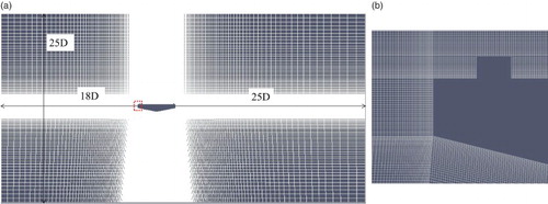
The domain was discretized spatially by a body-fitted mesh and the cell size was varied gradually with a geometric progression of 1.05 in all directions. The first cell height (y) away from the body, which was important for the correct computation of the viscous velocity profile, was selected such that the average y⁺ (y⁺ = ρyu*/μ, where u* is the friction velocity and μ is the dynamic viscosity) value lies below 5. For an R_e up to 6.0 × 10⁴, the average y⁺ value is around 2 and the maximum y⁺ value reaches up to 8.2. After close scrutiny we found that in a very small area near the edge of the leeward side curb, the y⁺ value reaches to the maximum value of 8.2, yet the y⁺ value in the remaining area was well below 5. Therefore, for this type of deck, only the average y⁺ value can provide meaningful information. For higher values of R_e (13 × 10⁴ and 20 × 10⁴) the first grid height (y) was decreased, yet the average y⁺ values reached 2.8 and 4.1, respectively. The grid system possessed a total of 108,778 and 224,546 elements for an R_e of 3.9 × 10⁴ and an R_e of 20 × 10⁴, respectively. The time step size (Δt = (C_oΔx)/U, where Δx is the smallest grid size) was calculated based on the Courant number (C_o). The maximum C_o was maintained around 0.5 for values of R_e up to 6.0 × 10⁴. For high values of R_e (20 × 10⁴), the solution became temporally expensive and the maximum C_o reached 1, yet the average C_o was well below 1 and the solution remained stable as 3 inner iteration loops were applied to the PISO algorithm.

As mentioned above, the first grid was placed in the viscous sublayer and stretched in all directions with a constant geometric progression of 1.05. It is important to check whether the solution was converged or not. A grid independency test was conducted for the pentagonal-shaped bridge deck having a θ of 14° and a side ratio (R) of 5 at an R_e of 6.0 × 10⁴. The static aerodynamic coefficients and Strouhal number (St_B) were taken as parameters of interest, as with Mannini et al. (2010). The definition of aerodynamic coefficients can be found in a later section. We adopted the standard methodology proposed by Roache (1998) to check the convergence of the grid system. The method is based on the Richardson extrapolation, where the finest grid is checked to see whether or not the grid has reached the asymptotic range of convergence (ARC). To apply the method, three grid systems are required, namely finest (1), medium, (2) and coarse (3) grids. The finest grid has the first grid height in the viscous sublayer with a geometric progression ratio of 1.05. The grid had a total 121,808 elements. We took two more grids with larger geometric progressions of 1.07 and 1.1. The medium and coarse grids had a total of 88,130 and 62,562 elements, respectively. We calculated the grid convergence index (GCI₁₂) for the finest (1) and medium (2) grids as follows: (4) where ϕ is the parameter of interest, F_S is the safety factor, r₂₁ is the refinement factor and P is the observed convergence rate. A safety factor of 1.25 was considered while the three grid systems were utilized. A refinement factor of 1.39 was used and P was calculated based on the prescribed equation given by Roache (1998, 1994). The function GCI₁₂ estimates the percentage of discretization error that remains in the finest grid (1) relative to the converged solution. Similar to Equation (4), a grid convergence index for the medium (2) and coarse (3) grids was also calculated (GCI₂₃). Finally, the following equation was utilized to check whether the finest grid solution reached the ARC: (5)

If Equation (5) yields a value of 1, this implies that the finest grid (1) reached the ARC. Table 1 displays the aerodynamic coefficients and S_tB for three considered grid systems, along with the grid convergence test results. As can be seen, the finest grid had a maximum error less than 5% and all the target parameters of interest nearly reached the ARC, while the S_tB exactly reached the ARC.

Table 1. Grid convergence study for pentagonal-shaped bridge deck with a θ of 14° at an R_e of 6.0 × 10⁴.

				Grid Convergence Test
Target parameter	Coarse grid (3)	Medium grid (2)	Finest grid (1)	GCI23 (%)	GCI12 (%)	ARC
Mean drag (CD)	0.64366	0.68075	0.69183	2.90	0.85	1.0162
RMS drag (CD')	0.02328	0.03165	0.03427	15.06	4.35	1.0827
Mean lift (CL)	−0.1124	−0.21144	−0.23497	18.24	3.90	1.1112
RMS lift (CL')	0.07647	0.125269	0.13832	17.78	4.31	1.1042
Mean moment (CM)	−0.10207	−0.09827	−0.09716	2.01	0.59	0.9886
RMS moment (CM')	0.014461	0.024463	0.027085	18.15	0.43	1.1072
Strouhal number (StB)	0.779	0.805	0.805	0	0	1

3. Performance of unsteady RANS

In this section the strength and efficiency of unsteady RANS is checked for a pentagonal-shape bridge deck to reproduce the flow field. Surface pressure and velocity distributions were considered as parameters of interest to check the performance of unsteady RANS. These two parameters are very common and useful for explaining various experimental results that are not fully understood. We conducted a simulation for the pentagonal-shaped bridge deck with a θ of 14° at an R_e of 6.0 × 10⁴ to maintain similarities with the experimental setup of Noda (2010). The curb angle (β) was set to 27°. Figure 3(a) shows the mean pressure distribution, along with the experimental result. The present simulation reproduced the trend of the surface pressure accurately, especially at the bottom-surface leading-edge and top-surface trailing-edge sides, where there was a very good comparison with the experimental work. Large discrepancies can be observed around the curb on the top deck and at the bottom deck trailing-edge side. In fact, a large flow separation occurred in those locations (Figure 4). As a consequence, the present simulation failed to capture the exact value of the pressure coefficients at those locations as the unsteady RANS performance deteriorates at the location of massive flow separation (Versteeg & Malalasekera, 2007). However, both at the top- and bottom-deck trailing-edge it could reproduce pressure recovery. The RMS of the surface pressure is plotted in Figure 3(b). In contrast to mean surface pressure, the discrepancy between the numerical and experimental work is higher in the case of RMS pressure. The present simulation failed to reproduce the trend in RMS pressure at the leading-edge side and underestimated the magnitude.

Figure 3. Surface pressure distribution around the pentagonal-shaped bridge deck: (a) mean pressure and (b) RMS pressure.

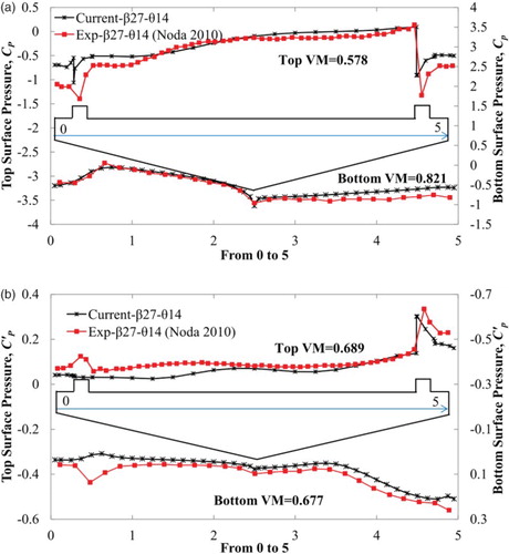
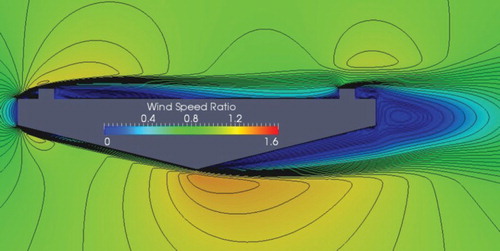
Figure 4. Wind speed ratio around the bridge deck for θ = 14°, R = 5, R_e = 20 × 10⁴.

In unsteady RANS, the fluctuating component is modeled based on two transport equations as discussed before, and the accuracy deteriorates for complicated geometry where massive flow separation occurs. This was also confirmed in past works (Mannini et al., 2010), in which unsteady RANS underestimated the response. Nevertheless, the RMS value of the pressure coefficient is a fairly sensitive quantity that depends on a number of experimental parameters (Bearman & Obasaju, 1982; Blevins, 1990; Mannini et al., 2009). However, the present simulation could reproduce the overall trend in RMS pressure distribution qualitatively and in a better way at the trailing-edge side top- and bottom-deck surfaces.

Up to this point we have only compared the results relatively. To check the level of accuracy and validate the numerical simulation we made comparisons with some standard validation metrics (VMs). A global VM was calculated based on the methodology presented by Oberkampf and Trucano (2002). The VM is straightforward; it takes the average of the number of experimental results at the discrete probing points and constructs a continuous cubic spline function. Then, the difference of the numerical and experimental functions is integrated all along the length. The VM has a maximum value of 1, and a value near to 1 is expected. However, the VM is conservative, as it takes the average of experimental results. The considered VM was as follows: (6) (7) where N is the number of experimental data, x_i represents the discrete probing locations along the body surface, L is the length of the body, φ represents the experimental results and ϕ represents the numerical results. The number of experimental data should be as high as possible in order to incorporate the influence of uncertainty. As we had only one set of data, we ignored the uncertainty. According to Oberkampf and Trucano (2002), when there is no uncertainty or error in the experimental data, the abovementioned equation can be simplified as follows: (8) where, I is the number of discrete probing locations. If the VM is calculated based on Equation (8) for a set of experimental and numerical data, the metric will estimate how closely the numerical result matches with the experimental one. A VM with a value of 1 indicates that the numerical results match completely with the experimental results. Figures 3(a and b) show the calculated VM based on Equation (8)(8) . The VM also reflects the general observations, as discussed in the previous chapter. The mean surface pressure has a higher metric value over the RMS surface pressure and mean bottom-surface pressure over the top surface. The bottom-surface mean pressure has the highest metric value of 0.821, and the other metric values are also well above 0.5.

The velocity is another important parameter that explains the aerodynamics of the bluff body, along with the pressure plot. The wind-speed ratio plot around the selected deck section is shown in Figure 4, where the simulation inlet velocity was used to normalize the local velocity. In previous work, Noda (2010) conducted a PIV experiment for the same deck shape with a θ of 14° and plotted the wind-speed ratio at an R_e of 21 × 10⁴. To increase the compatibility of the comparison, the simulation was conducted again with an R_e of 20 × 10⁴. Figure 5 shows the previous experimental PIV result. By comparing Figures 4 and 5, it can be seen that the present simulation can reproduce the overall and general tendency of the velocity distribution very close to the experimental one. Even the velocity acceleration on the top of the curb and at the bottom-surface mid-deck is also captured very well. However, the numerical wake size is bit larger than the experimental one. By observing the velocity we assume that the flow first separates at the top-deck leading edge just after the curb and at the bottom deck on the trailing-edge side. The leading-edge top-deck separated shear layer plays an important role in destabilizing the bridge (Kubo et al., 1992; Nakamura & Nakashima, 1986), while the bottom-deck trailing-edge separation increases the vortex shedding tendency and the after-body wake size. In Figure 4 a very clear large wake zone can be observed. In this section we found that unsteady RANS could predict some important flow features with reasonable accuracy. In the following section, we explore how the variation of θ affects these flow features.

Figure 5. Wind speed ratio around the bridge deck for θ = 14°, R = 5, R_e = 21 × 10⁴ by PIV experiment (Noda, 2010). Figure 5 Note: In experimental the work, the same color bar level was used as for the numerical work (0–1.6).

4. Influence of the bottom-plate slope

In this section, the effect of the θ of a pentagonal-shaped bridge deck on the aerodynamic coefficients and flow field is demonstrated numerically at an R_e of 3.9 × 10⁴. Kubo et al. (2007) utilized three β of 27°, 30° and 33° to check the performance of SIM on critical flutter wind-speed. Therefore, we also checked three β of 27°, 30° and 33° and the curb height (h/B) was set to 0.025. The θ was varied from 10° to 16° by varying the values of R from 6.45 to 4.75, respectively. The depth (D) of the deck was varied to alter the θ without changing the width (B) and the side depth (a/B) of the deck. The a/B ratio was set to 0.067. In past experimental work (Kubo et al., 2007; Yoshida et al., 2006), the θ was varied by following the same procedure. These results may have an effect of R, however, so to maintain coherence with past experimental work, the same procedure was chosen. The aerodynamic coefficients such as drag (C_D), lift (C_L), moment (C_M) and S_tB were defined as follows: (9) (10) (11) (12) where F_D, F_L and F_M are the drag, lift and moment forces acting per unit length on the bridge deck respectively, and f is the shedding frequency. The mean and RMS values of the aerodynamic coefficients when varying the θ are plotted in Figure 6. As can be seen, β does not significantly affect the aerodynamic coefficients. However, the smaller β of 27° has less of an aerodynamic response. Kubo et al. (2007) also found that a β of 27° had a slightly higher critical flutter wind-speed than the other values of β.

Figure 6. Influence of θ on the aerodynamic response for various values of β at an R_e of 3.9  × 10⁴.

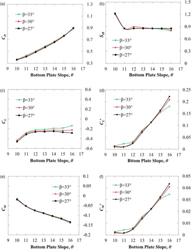
Figure 6 also shows that the θ has a greater influence on the aerodynamic coefficients than β. Regardless of β, the smaller θ results in lower magnitudes of the aerodynamic coefficients. For any value of θ from 16° to 10°, the deck experiences a negative lift. In Figures 6(d and f), the RMS values of lift and moment decrease significantly as the θ decreases. Basically, the RMS value of the aerodynamic coefficients is an overall or general indicator of the dynamic behavior of a bluff body. Therefore, a deck with a smaller RMS value would imply a better dynamic behavior, as the flow can move smoothly around the deck. In the literature, experimental data of flutter wind-speed for varying the θ is available; hence, we took this opportunity to compare the trend in the result with the literature. Past experimental work has shown that flutter wind-speed increases as the θ decreases, and that vortex shedding instability stops when the θ is less than 19° (Kubo et al., 2007; Noda, 2010; Yoshida et al., 2006). Figure 7 shows that for a deck with a β of 30°, the reduced flutter wind-speed increases as the θ decreases. The present RMS value of lift and moment has similar trends in the result of the flutter wind-speed obtained previously (Kubo et al., 2007; Yoshida et al., 2006). With this established, we started to explore the flow field to understand the trend found in both the numerical and experimental results.

Figure 7. Influence of θ on flutter speed (V/fB) for a β of 30° by experimental work (Kubo et al., 2007; Yoshida et al., 2006).

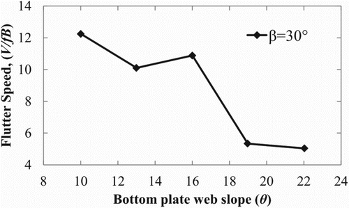
Figure 8. Mean surface pressure distributions around the bridge deck section with a β of 27° for various values of θ.

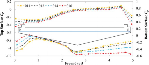
Figure 9. RMS surface pressure distributions around the bridge deck section with a β of 27° for various values of θ.

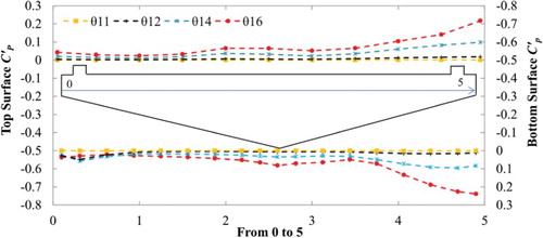
The mean and RMS values of surface-pressure distribution of the selected deck section with a θ of 11°, 12°, 14° and 16° are plotted in Figures 8 and 9, respectively. In the case of mean surface-pressure the bottom-deck pressure is more influential than the top-deck surface when the bottom-deck slope is altered. The mean surface-pressure distribution is mainly affected at the leading and trailing edges of the deck due to the variation in θ. As the θ decreases (as the a/D ratio increases) the bottom-deck leading-edge side negative-pressure area increases and the trailing-edge side negative-pressure area decreases. Basically, this kind of negative pressure indicates the separation of the shear layer from the deck surface. Based on the mean surface pressure the trend in aerodynamic coefficients can also be explained. For example, for a small θ (11°), the deck experiences an increased downward force (negative pressure increases) at the leading-edge side bottom-surface and a decreased downward force (negative pressure decreases) at the trailing-edge side bottom-surface. As a result, the overall positive moment (anticlockwise) tendency of the deck increases. Similarly, as the leading-edge side negative pressure increases, the negative lift (downward) value tendency increases for a small θ of 11°. Unlike the mean surface-pressure, the RMS pressure is actually affected at the trailing-edge side (Figure 9). As the θ decreases, the trailing-edge side RMS value also decreases. This implies that the fluctuation of pressure is influenced by the after-body vortex activity. To understand the pressure fields further, the velocity fields around the decks were explored.

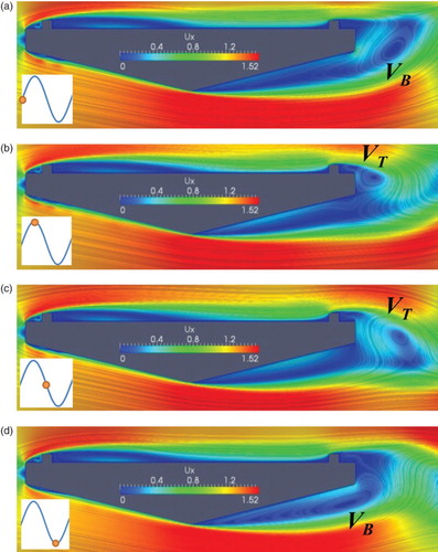
The instantaneous velocity field along one lift cycle is plotted for a deck with a θ of 14° in Figure 10. The after-body vortex can clearly be seen, and good correlation was found between the vortex location and the lift magnitude. In Figure 10(b), as the top vortex (V_T) forms, the deck experiences the maximum lift force (upward), while the deck experiences the minimum lift force (downward) as the bottom vortex (V_B) forms (Figure 10(d)) very close to the trailing-edge bottom-deck surface. This confirms that the after-body vortex shedding is the main cause of fluctuating aerodynamic coefficients.

Figure 10. Instantaneous velocity field for deck shape having a θ of 14° along one lift cycle at (a) 0°, (b) 90°, (c) 180°, and (d) 270°.

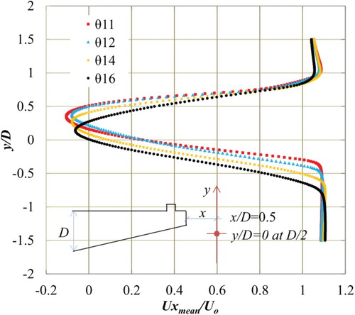
Figure 11 shows the mean velocity field normalized with the inlet velocity along with contour lines. The velocity distribution agrees well with mean pressure distribution (Figure 8) and makes it easier to understand the mean and RMS pressure distribution. The wake size decreases as the θ decreases and the deck experiences smaller RMS fluctuations. The reason for a smaller wake size at a smaller θ is due to the decrease of the trailing-edge side flow separation. As a result, the vortex may form just after the deck with a smaller size rather than very close to the trailing-edge bottom-deck surface, as shown in Figure 10(d). A similar observation was made by Larsen and Wall (2012) for a streamlined bridge deck. It was shown that for a small θ the trailing edge flow separation decreases and the vortex forms away from the deck. Figures 12 and 13 display the velocity distribution at the trailing edge and 0.5D downstream of the deck. The flow separation can clearly be seen at the trailing edge and gradually decreases as the θ decreases. Thus the wake size decreases, as shown in Figure 13. As a result, both the drag and the RMS value of aerodynamic coefficients decreases, implying that a deck with a smaller wake may require a greater wind-speed for flutter to occur. However, this is just conjecture based on the present observations and demands more elaborate investigation. In this section we have highlighted some trends in the aerodynamic coefficients and clarified them through an analysis of the pressure and velocity distributions. However, the trend we found both in terms of the aerodynamic coefficients and flow field is for a specific R_e, thus, an investigation is needed in order to understand how the obtained trend in the results changes when the wind velocity increases. In the following section, we attempted to gain insight into the effect of the R_e on the flow field for a pentagonal-shaped bridge deck.

Figure 11. Wind speed ratio around the bridge deck where the θ is (a) 16°, (b) 14°, (c) 12°, and (d) 11°.

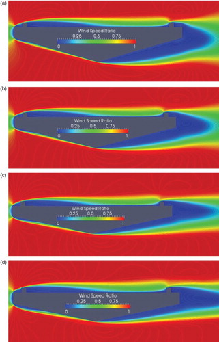
Figure 12. Velocity distributions at the trailing edge for various values of θ.

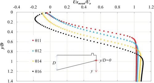
Figure 13. Velocity distributions at the wake for various values of θ.

5. Influence of the Reynolds number

The influence of the R_e is a widely-discussed topic in the bridge and bluff body aerodynamics fields. It is always important to know how the R_e affects the aerodynamic response. However, it is impossible to reproduce the influence of a natural wind R_e, as it is quite high. In a wind tunnel we can generate a reasonable value of R_e. In numerical analysis, this problem becomes even worse. Basically, at high wind-speeds, large numbers of grids are required to model the thinner boundary layer accurately, and the time step also becomes smaller. Therefore, the computational load becomes huge. It would be an ambitious job to investigate the effects of a very high R_e on a bridge deck. In the present work we considered five different R_e (2 × 10⁴–20 × 10⁴) to show the trend in the results, particularly its influence on the mean aerodynamic coefficients and the flow field. The R_e was defined in terms of the width (B) of the bridge deck. Simulations were conducted for one specific deck shape with an R of 5 and a θ of 11°, as a smaller θ possess better aerodynamic behavior. The R_e was increased by increasing the inlet velocity and keeping the dimension of the bridge decks same.

Figure 14 shows the influence of the R_e on the aerodynamic coefficients; the dependency of the response on R_e can be clearly seen. Both the mean and RMS response become almost independent of the R_e for a value higher than 13 × 10⁴. The mean value gradually decreases as the R_e increases until a value of 13 × 10⁴, then becomes stable. The lift coefficient remains negative as the R_e increases. It is good that at a higher velocity the bridge will experience even larger downward forces, increasing the total stiffness of the bridge system. In the present work we tried to focus on some important aerodynamic features such as the leading-edge top-deck separation and the bottom-deck leading- and trailing-edge separation. Figure 15 represents the mean velocity distribution for three values of R_e. As can be seen, the increase in R_e affects the flow field noticeably in the high R_e range (≥13 × 10⁴). The top-deck shear layer separation length decreases as the R_e increases. The decrease in the top-deck separation length strengthens the concepts of SIM, even at high wind-speeds.

Figure 14. R_e influence on (a) mean and (b) RMS values of aerodynamic coefficients for a deck where θ = 11°, β = 30°, and R = 5.

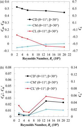
Figure 15. Wind speed ratio around the bridge deck with where θ = 11° and R = 5 for (a) R_e = 1.9 × 10⁴, (b) R_e = 6.0 × 10⁴, and (c) R_e = 13 × 10⁴.

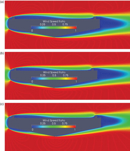
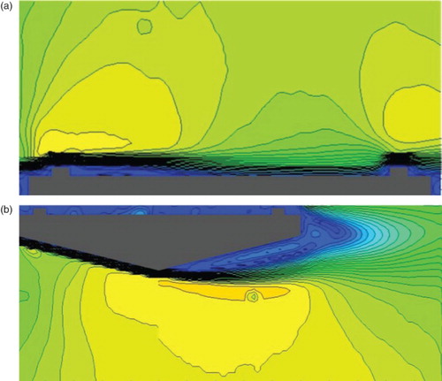
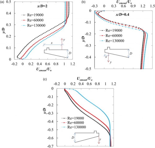
On the other hand, at the bottom deck the leading-edge side separation increases, yet the trailing-edge separation decreases. To clarify these kinds of phenomena, the velocity distributions are plotted at three different locations in Figure 16. Both at the top-deck leading-edge side and bottom-deck trailing-edge side the flow separation can be seen for small values of R_e, yet the flow separation decreases and stops at high values of R_e. However, the bottom-deck leading-edge side separation increases with increases in R_e. This increase in bottom-deck leading-edge separation and decrease in top-deck leading-edge separation increases the downward lift force, while the decrease in bottom-deck trailing-edge flow separation reduces the after-body wake size and directly affects the mean drag value, resulting in a smaller value. Similar phenomena were observed by Schewe (2001), where an oil-flow experiment was conducted for a bluff bridge deck section in a wind tunnel. It was found that at high values of R_e (1.5 × 10⁶) the top-deck leading-edge and the bottom-deck trailing-edge flow separation decreases, decreasing the drag of the section.

Figure 16. Velocity distributions for the pentagonal-shaped bridge deck at (a) the top-deck leading-edge, (b) the bottom-deck leading-edge, and (c) the bottom-deck trailing-edge.

Further, in section 3 we found that a θ of 11° has the least RMS response due to a small trailing-edge flow separation at an R_e of 3.9 × 10⁴. At a high value of R_e (13 × 10⁵), the trailing-edge flow separation stops completely and forms a boundary layer (Figure 16(c)). Based on this explanation it can be presumed that at a higher R_e (20 × 10⁴), the separation may stop at a θ greater than 11°. As a result, the drag decreases due to the decrease in relative wake size (as a larger θ has a smaller a/D ratio). Therefore, at a high R_e (≥20 × 10⁵), the optimum aerodynamic response can be found at a θ greater than 11°. This could be a possible explanation why Kubo et al. (2007) obtained less of a drag force at a θ of 12°.

6. Conclusions

A numerical investigation was carried out for an aerodynamically stable pentagonal-shaped bridge deck where the curb on the top deck controls the flow pattern, which is known as SIM. The efficiency of the unsteady RANS simulation was checked through attempting to reproduce the aerodynamic responses for this kind of shape and comparing the results with past experimental work. It was also intended to explore the important flow features of the pentagonal-shaped bridge deck which govern the response and the flow field. A further aim was to demonstrate how the variation of the θ and R_e affects those flow features and aerodynamic responses of the bridge deck.

We found that an unsteady RANS simulation can reproduce the aerodynamic characteristics reasonably well for the considered deck shape. It can capture the general trend in the results. Discrepancies were noticed at the location where large flow separation occurs; it yields the target mean value qualitatively in those locations, yet underestimates the RMS value noticeably. However, the unsteady RANS simulation captures the velocity field and flow pattern very accurately compared to the experimental results. Therefore, further application of unsteady RANS to experimental work is encouraged in order to analyze the flow around bridge decks to better understand the aerodynamic response.

The pentagonal-shaped bridge deck has improved aerodynamic behavior. We found that the most important flow features are the top-deck leading-edge side flow separation and the bottom-deck leading- and trailing-edge side flow separation. The leading-edge side top and the bottom-deck separation affects mainly the mean values of aerodynamic coefficients, yet the trailing-edge flow separation affects both the mean and the RMS values of aerodynamic coefficients. Like the previous experiments, we also found that smaller values of β and θ result in better aerodynamic behavior. In summary, at a small θ the bottom-deck trailing-edge side flow separation decreases and the wake size reduces, improving the aerodynamic behavior of the deck. At the present R_e (3.9 × 10⁴) the trailing-edge flow separation stops at a θ of 11°. However, at a high value of R_e (≥10⁵) the flow separation may stop at a θ greater than 11°.

The increase in R_e increased the bottom-deck leading-edge side flow separation and decreased both the top-deck leading-edge side and bottom-deck trailing-edge side flow separation up to an R_e of 13 × 10⁴. Beyond this value of R_e the flow field and the aerodynamic coefficients become less sensitive to R_e. Therefore, for this kind of pentagonal-shaped bridge deck an investigation should be carried out higher than that range, otherwise the results may have some R_e effects. Further, the present simulations also showed that the SIM becomes even more effective at higher values of R_e. In the present work we found some important flow features that control the static aerodynamic response of the deck and after-body vortex shedding activity. Future work will try to clarify how these flow features contribute to the dynamic behavior (vortex shedding and flutter instability) of the deck and their relative importance.

Disclosure statement

No potential conflict of interest was reported by the authors.

References

- Bearman, P. W., & Obasaju, E. D. (1982). An experimental study of pressure fluctuations on fixed and oscillating square-section cylinders. Journal of Fluid Mechanics, 119, 297–321. doi:10.1017/S0022112082001360
- Blocken, B. (2014). 50 years of computation wind engineering: Past, present and future. Journal of Wind Engineering and Industrial Aerodynamics, 129, 69–102. 2014. 10.1016/j.jweia.2014.03.008
- Blevins, R. D. (Eds.). (1990). Flow-induced vibration (2nd ed.). Florida, USA: Krieger Publishing Company, Malabar.
- Bruno, L., & Mancini, G. (2002). Importance of deck details in bridge aerodynamics. Structural Engineering International, 12(4), 289–294. Retrieved from http://www.iabse.org/IABSE/Publications/SEI_Journal/IABSE/publications/SEI_Journal/SEI_Journal.aspxhttp://www.iabse.org/IABSE/Publications/SEI_Journal/IABSE/publications/SEI_Journal/SEI_Journal.aspx doi: 10.2749/101686602777965234
- Brusiani, F., De Miranda, S., Patruno, L., Ubertini, F., & Vaona, P. (2013). On the evaluation of bridge deck flutter derivatives using RANS turbulence models. Journal of Wind Engineering and Industrial Aerodynamics, 119, 39–47. doi:10.1016/j.jweia.2013.05.002
- Franke, J., Hellsten, A., Schlünzen, H., & Carissimo, B. (Eds.). (2007). Best practice guideline for the CFD simulation of flows in the urban environment. COST Office Brussels, Belgium. ISBN 3-00-018312-4, 2007.
- Huang, L., & Liao, H. (2011). Identification of flutter derivatives of bridge deck under multi-frequency vibration. Engineering Applications of Computational Fluid Mechanics, 5(1), 16–25. 2011. doi:10.1080/19942060.2011.11015349
- Issa, R. I. (1986). Solution of the implicitly discretized fluid flow equations by operator-splitting. Journal of Computational Physics, 62, 40–65. Retrieved from http://www.sciencedirect.com/science/article/pii/0021999186900999
- Kelkar, K. M., & Patankar, S. V. (1992). Numerical prediction of vortex shedding behind a square cylinder. International Journal for Numerical Methods in Fluids, 14, 327–341. doi:10.1002/fld.1650140306
- Kubo, Y., Hayashida, K., Noda, T., & Kimura, K. (2008). Mechanism on reduction of aerodynamic forces and suppression of aerodynamic response of a square prism due to separation interface method. In Proceedings of 6th Int. Colloq. On Bluff Body Aerodynamics and Applications, 20–24 July, Milano, Italy, 1–4.
- Kubo, Y., Hirata, K., & Mikawa, K. (1992). Mechanism of aerodynamic vibrations of shallow bridge girder sections. Journal of Wind Engineering and Industrial Aerodynamics, 42, 1297–1308. Retrieved from http://www.sciencedirect.com/science/article/pii/016761059290138Z
- Kubo, Y., Yoshida, K., Tuji, E., Kimura, K., & Kato, K. (2007). Development of aerodynamically stable bridge girder cross section for long span bridges. In proceedings of 12th Int. Conf. on Wind Engineering, 1–6 July, Cairns, Australia, pp. 239–246, 2007.
- Larsen, A., & Wall, A. (2012). Shaping of bridge box girders to avoid vortex shedding response. Journal of Wind Engineering and Industrial Aerodynamics, 104–106, 159–165. doi:10.1016/j.jweia.2012.04.018
- Mannini, C., Soda, A., & Schewe, G. (2010). Unsteady RANS modelling of flow past a rectangular cylinder: Investigation of Reynolds number effects. Computers and Fluids, 39(9), 1609–1624. doi:10.1016/j.compfluid.2010.05.014
- Mannini, C., Soda, A., Voß, R., & Schewe, G. (2010). Unsteady RANS simulation of flow around a bridge section. Journal of Wind Engineering and Industrial Aerodynamics, 98(12), 742–753. doi:10.1016/j.jweia.2010.06.010
- Mannini, C., Weinman, K., Soda, A., & Schewe, G. (2009). Three-dimensional numerical simulation of flow around a 1:5 rectangular cylinder. In C. Borri, G. Augusti, G. Bartoli, & L. Facchini (Eds.), Proceedings of Fifth European and African Conference on Wind Engineering. Florence, Italy: Firenze University Press. 2009.
- Menter, F. R. (1994). Two-equation eddy-viscosity turbulence models for engineering applications. AIAA Journal, 32(8), 1598–1605. doi:10.2514/3.12149
- Nakamura, Y., & Nakashima, M. (1986). Vortex excitation of prism with elongated rectangular, H and (Vertical, Dash) cross-sections. Journal of Fluid Mechanics, 163, 149–169. http://dx.doi.org/10.1017/S0022112086002252
- Nieto, F., Kusano, I., Hernandez, S., & Jurado, J. A. (2010). CFD analysis of the vortex-shedding response of twin-box deck cable-stayed bridge. In Proceedings of 5th Int. Symp. on Computational Wind Engineering, 23–27 May, North carolina, USA, 1–8.
- Noda, T. (2010). Study on development of narrow width deck section for suspension bridge. PhD dissertation, Graduate school engineering, Kyushu Institute of Technology, Japan, (Japanese).
- Noda, T., Kubo, Y., Kimura, K., Kato, K., Okubo, K., & Yoshida, K. (2009). The effects of lower flange slope on the aerodynamic stability of a pentagonal cross-section girder. Journal of Civil Engineering (JSCE), 65(3), 797–807 (Japanese).
- Oberkampf, W. L., & Trucano, T. G. (2002). Verification and validation in computational fluid dynamics. Progress in Aerospace Sciences, 38, 209–272. 10.1016/S0376-0421(02)00005-2
- Roache, P. J. (1994). Perspective: A method for uniform reporting of grid refinement studies. Journal of Fluids Engineering, 116(3), 405–413. doi:10.1115/1.2910291
- Roache, P. J. (1998). Verification and validation in computational science and engineering. Albuquerque, New Mexico: Hermosa Publishers.
- Šarkić, A., Fisch, R., Höffer, R., & Bletzinger, K. (2012). Bridge flutter derivatives based on computed, validated pressure fields. Journal of Wind Engineering and Industrial Aerodynamics, 104–106, 141–151. doi:10.1115/1.2910291
- Sarwar, M. W., & Ishihara, T. (2010). Numerical study on suppression of vortex-induced vibrations of a box girder bridge section by aerodynamic countermeasures. Journal of Wind Engineering and Industrial Aerodynamics, 98, 701–711. doi:10.1016/j.jweia.2008.02.015
- Sarwar, M. W., Ishihara, T., Shimada, K., Yamasaki, Y., & Ikeda, T. (2008). Prediction of aerodynamic characteristics of a box girder bridge section using the LES turbulence model. Journal of Wind Engineering and Industrial Aerodynamics, 96, 1895–1911. doi:10.1016/j.jweia.2008.02.015
- Schewe, G. (2001). Reynolds-number effects in flow around more-or-less bluff bodies. Journal of Wind Engineering and Industrial Aerodynamics, 89, 1267–1289. 10.1016/S0167-6105(01)00158-1
- Shirai, S., & Ueda, T. (2003). Aerodynamic simulation by CFD of flat box girder of super-long span suspension bridge. Journal of Wind Engineering and Industrial Aerodynamics, 91, 279–290. doi:10.1016/S0167-6105(02)00351-3
- Sohankar, A., Davidson, L., & Norberg, C. (1995). Numerical simulation of unsteady flow around a square two-dimensional cylinder. In Proceedings of Twelfth Australasian Fluid Mechanics Conference, 10–15 December, Sydney, Australia, 517–520.
- Sohankar, A., Davidson, L., & Norberg, C. (1998). Low- Reynolds- number flow around a square cylinder at incidence: study of blockage, onset of vortex shedding and outlet boundary condition. International Journal for Numerical Methods in Fluids, 26, 39–56. 10.1002/(SICI)1097-0363(19980115)26:1<39::AID-FLD623>3.0.CO;2-P
- Sweby, P. K. (1984). High resolution schemes using flux limiters for hyperbolic conservation laws. SIAM Journal on Numerical Analysis, 21, 995–1011. 10.1137/0721062
- Versteeg, H., & Malalasekera, W. (Eds.). (2007). Chapter 3: An introduction to computational fluid dynamics: The finite volume method. (2nd ed.). London: Pearson.
- Watanabe, S., & Fumoto, K. (2008). Aerodynamic study of a slotted box girder using computational fluid dynamics. Journal of Wind Engineering and Industrial Aerodynamics, 96, 1885–1894. doi:10.1016/j.jweia.2008.02.056
- Yoshida, K., Kubo, Y., Tsuji, E., Kimura, K., & Kato, K. (2006). Effects of lower plate slope on the aerodynamic characteristics of a pentagonal cross section bridge deck. Proceedings of 19th National Symposium on Wind Engineering, Japan, 295–300.