Numerical and experimental hydrodynamic study of a coolant distributor for grinding applications

ABSTRACT

In grinding, the high frictional energy is converted into heat, which may cause thermal damage and degradation of the wheel and the workpiece. Unwanted thermal effects must thus be reduced, often by external cooling using a curved-duct coolant distributor to match the wheel geometry. The performance of such a system depends strongly on the impinging jet flow properties to ensure efficient sprinkling of the hot spots. The fluid distributor, placed above the workpiece, is pierced with a certain number of identical nozzle fittings, providing multiple jets at the outlet of the nozzles. These jets sprinkle the solids over a given zone and remove the heat by convective transfer. The cooling is hence dependent on the flow structure, meaning the jet diameters, trajectories and velocities, determined up-flow by the distributor design. The present study is devoted to the hydrodynamics aspects of the fluid distributor, aiming to determine the flow-rate distribution at the different orifices and the flow-rate–pressure relationship, for a variety of nozzle diameters and feeding flow rates, under isothermal conditions. A simple hydraulic balance in the device was not able to predict with sufficient accuracy the actual measurements, even when the Venturi effect was accounted for. This discrepancy is due to the curvature of the distributor, inducing secondary flows in interaction with the nozzle outlets, which leads to a rather complex flow pattern. To overcome this issue, a computational fluid dynamics (CFD) tool was used and compared with in situ experiments – global flow rate and pressure measurements were additionally taken with particle image velocimetry (PIV) to gain insight into the local structure. Simulations were performed with a 3D turbulence model for Reynolds numbers up to 100,000. This model provides an efficient tool for coupling with the thermal study at a later step, allowing global sizing and energetic optimization of the grinding process.

KEYWORDS:

• U-bend
• sprinkling jet
• CFD
• cooling system
• multiple outlets
• grinding

1. Introduction

Cooling by sprinkling jets is a highly efficient technique used in various types of machinery applications, including the tempering and shaping of glass, the annealing of metals, the drying of textiles, gas turbine blade cooling, electronic equipment, and especially grinding (Goldstein & Seol, 1991; Lytle & Webb, 1994; Wei, Zhang, Li, & Wang, 2015; Womac, Ramadhyani, & Incropera, 1993).

Previous studies on different types of impinging-jet cooling systems show that the local heat and mass transfer depends on geometric and hydrodynamic factors such as nozzle location and shape, jet velocity and turbulence level, surface spacing, jet orientation and the surrounding conditions (Aziz, Raiford, & Khan, 2008; Jaramilloa, Pérez-Segarraa, Rodrigueza, & Olivaa, 2008; Ockfen & Matveev, 2009).

The sprinkling onto the workpiece is hence governed by the flow outlet conditions in the coolant distributor, which are the result of the hydrodynamic conditions in the latter. The hydrodynamic study of the fluid distributor is the first stage of a project conceived with the aim of optimizing the cooling process, and is the topic of the present paper. The second stage is to analyze the heat transfers at the workpiece/wheel contact in the different media – grinding wheel, workpiece, air and fluid – for different jet characteristics. The details of this work, based on the use of innovative thermal sensors able to withstand the wheel's high speed, can be found in Moussa, Garnier, and Peerhossaini (2015a). The heat-transfer analysis for the grinding wheel has already been investigated elsewhere (Moussa, Garnier, & Peerhossaini, 2013) and an analysis of the interfacial parameters (heat flux, thermal contact resistance, etc.) will be the subject of a future publication. An overview of this study can be found in Moussa, Garnier, and Peerhossaini (2015b). The results of both studies will be combined to propose an optimized configuration, consisting of defining the distributor design and the operating conditions required for generating a more efficient jet system which naturally accounts for the energy cost. Various criteria can be used for this optimization and this issue will be treated in a future work.

With respect to the hydrodynamic problem, the aim is to understand how the flow rate is shared between the different orifices to generate the jet system and establish the flow-rate–pressure relationship relative to the geometry of the nozzles. This aspect is of great importance for the efficiency of the process, beyond the size of the pump. A simple hydraulic balance coupled with the mass balance is insufficient for accurately predicting the required flow features in this configuration due to the flow complexity that results from the curvature of the channel and the vortices at the orifices.

Due to the need for better knowledge with respect to the flow, a local analysis of the flow was conducted via simulation using the computational fluid dynamics (CFD) software program ANSYS Fluent and in situ experiments using particle image velocimetry (PIV). For this task, a special optical model of the distributor on a 1:1 scale was built.

Flows induced by streamline curvatures are well known by their enhancement of the transverse fluid motion, mass transfer and pressure drop (Momayez, Dupont, Delacourt, Lottin, & Peerhossaini, 2009; Momayez, Dupont, Delacourt, & Peerhossaini, 2010; Momayez, Dupont, & Peerhossaini, 2004a, 2004b; Peerhossaini & Bahri, 1998). Flows in a U-bend have also been studied numerically and experimentally for gas and liquid flows (Hidayat & Rasmuson, 2004; Kim, Yadav, & Kim, 2014). Numerous models based on eddy viscosity models or Reynolds stresses models (RSMs) have been investigated (Iacovides, Launder, & Li, 1996a, 1996b). Here, we used the k-ε approach based on the Boussinesq hypothesis (Hinze, 1975).

The paper is presented in three parts. Firstly, the coolant distributor and the main elements of the grinding process are presented. Secondly, the dimensions of the distributor are presented, as well as the experimental benchmark and the measurement techniques used, including the PIV settings. The numerical method and turbulence model are also detailed. Thirdly, the numerical and experimental results are shown with validation based on the pressure drop and flow-rate measurements along the distributor. The paper is concluded with an overview of the future steps in the process of optimizing the actual distributor.

2. Materials and methods

2.1. Coolant distributor geometry

A schematic diagram of the test section (distributor geometry) is presented in Figure 1(a). The distributor has three main parts: the entrance section, the curved duct, and the nozzles extending from the bottom of the curved duct. The different elements (tool, workpiece, coolant distributor) of the grinding process are shown in Figure 1(b).

Figure 1. (a) 2D view of the distributor geometry; (b) different elements of the grinding process.

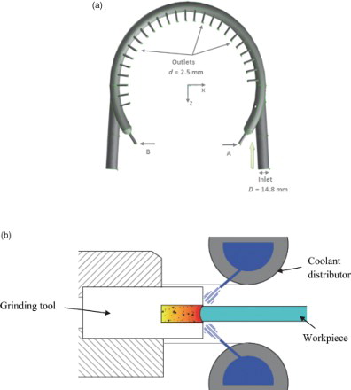
The entrance to the curved duct is a tube with a circular cross-section of diameter D = 14.8 mm. The entrance section is the intersection of the entrance pipe and the curved-duct section and is of an elliptic shape. The curvature ratio of the duct is Rc/D = 7.5. The curved section has a rectangular cross-section of height h = 26 mm and width w = 12.3 mm. In the standard geometry, the flow exits through multiple nozzles of 2.5 mm diameter which extend from the bottom of the curved section, providing the coolant free jets, although different nozzle diameters are investigated in the CFD study (see section 3.1.1).

2.2. Flow loop

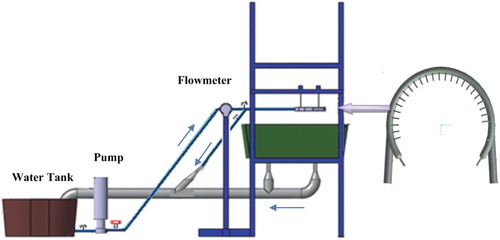
The flow loop comprises two water tanks, one of 1 m³ volume for water feeding and the other for discharge (Figure 2). Water is circulated in a closed loop by a centrifugal pump allowing a maximum pressure head of 1.2 MPa. The flow at the inlet of the pre-conditioner tube (upstream of the test section) is controlled by a magnetic flowmeter. Flexible tubes of 34 mm inner diameter and 4 mm thickness are used for piping. An 800 W surface pump drains the main tank. The coolant distributor is mounted on an aluminum support platform. An anti-splash system prevents water projected by the jets from hitting the drain box bottom and protects the PIV optics.

Figure 2. Experimental setup of the distributor hydraulic loop.

2.3. PIV measurement techniques

PIV was used to measure the mean and fluctuating velocity components (for a review, see Prasad, 2000).

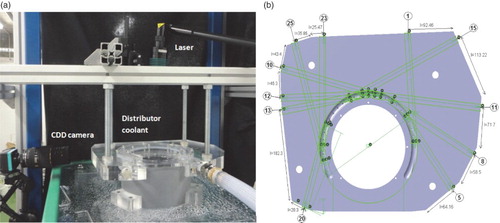
In the present study, the PIV system is composed of a pulsed Neodymium Yttrium Aluminum Garnet laser for illumination, a recording medium, a Charge-Coupled Device camera to capture the particle movements in the flow, seeding particles, and a PC platform for data recording and analysis (Figure 3(a)). Plane optical windows are implemented to obtain a clear image without diffraction effects. The top view of the Poly(methyl methacrylate) distributor presented in Figure 3(b) shows the different observation planes numbered from 1 to 25. Every plane corresponds to the vertical section above the nozzle (1 to 25). The arrows indicate the location at which each image is taken. The flow was visualized laterally (vertical light sheet).

Figure 3. (a) Experimental and PIV setup; (b) test section.

The recordings and data analyses were performed using the Dantec Dynamic software. The experiments were carried out using standard curved-duct geometry (inlet diameter D = 14.8 mm and nozzle diameter d = 2.5 mm). Some parts of the detected images have been masked and deleted due to light reflection and aberrant velocity vectors. This image processing caused a loss of 5–15% of the real images. Despite this it was possible to compare three experimental images of three main sections to the numerical ones. The intrinsic error of the PIV method, due to the image sampling and processing, is generally considered within 5–10%, depending on the local velocity magnitude.

The operating conditions are listed in Table 1 but for brevity, the PIV results are only presented for an inlet flow rate of Q = 3.8 m³/h.

Table 1. Parameters for PIV acquisition.

Parameters	Adaptation
Method of correlation	Intercorrelation
Laser	Wave length = 532 nm
Particles	Hollow glass spheres: diameter = 10 μm; density = 1.1 g/cm^3; refractive index = 1.52
Dimension of ZI and pixels	64 × 64 pixels; 1 pixel = 0.019 mm
	Lint = 64 × 0.019 mm
Number of images	n = 100
Time between two laser pulsations Δt	Δt = 30, 40 and 70 μs
Recovery	50%
Time between two image pairs	0.067 s

2.4. Other experimental settings

For the purpose of experimental validation, the pressure was measured at different locations along the curved duct by a Digitron differential pressure gauge which allowed a pressure range from 1 mbar to 2 bar. The systematic error of this pressure gauge given by its technical guide for the measurement interval is 0.46%. A conventional volumetric method was used to measure the jet flow rates. The inlet flow rate was measured by a magnetic flowmeter (Coriolis mass flow measurement from Endress+Hauser) with a 1% error margin.

2.5. Numerical approach

The steady-state incompressible Navier–Stokes and continuity equations in curved ducts were solved using Fluent v6.3 (ANSYS, 2006). Among several models from the Fluent library, the realizable k-ε model is one of the most accurate models for predicting turbulence phenomena in curved ducts (Launder & Spalding, 1972), and was used in the simulation. Davis, Rinehimer, and Uddin (2012) have demonstrated that this model has a superior ability to capture the mean flow of complex structures measured in experimental data in their study about wall-mounted square cylinders. The difference between the standard k-ε model and the realizable one lies in the eddy viscosity formulation and the turbulence kinetic energy (TKE) dissipation. This model is accurate, especially in boundary layers and high shear regions. Nevertheless, it does not account for the anisotropy of the flow and is not able to provide a refined turbulence structure description – but we have validated the use of this model as it provides fair predictions of the global phenomena which we want to observe, meaning the flow-rate distribution at the nozzles and the flow-rate–pressure relationship.

Mean velocity and turbulence intensity are specified at the inlet (as derived from Hinze, 1975). The two-layer model was used to compute the wall region. No-slip and no-penetration conditions were prescribed at the wall. A pressure outlet condition was used at the exits of the nozzles distributed along the curved duct; the pressure value was set to zero. The working fluid was tap water with no additives.

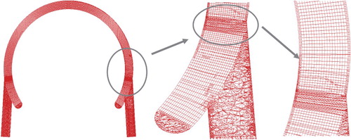
An unstructured 3D mesh with hexahedral and tetrahedral cells was adopted and refined at the solid boundaries (Figure 4). An appropriate meshing was found with approximately 1,380,030 cells. The skew equiangle parameter shows that the worst element is about 0.85. Better convergence of results was obtained by using the Cooper algorithm for volume meshing.

Figure 4. Refined tetrahedral mesh in the wall region.

In pressure–velocity coupling, the SIMPLEC algorithm was used and a convergence criterion of 10⁻⁵ was adopted.

3. Results and discussion

3.1. Numerical results

3.1.1. Operating conditions

Different configurations were studied numerically, corresponding to the experimental conditions. At the inlet, two flow rates were considered: Q = 3.8 and Q = 6. For Q = 3.8 m³/h, the mean jet exit velocities along the distributor were 3.2 m/s, 8.87 m/s and 85.9 m/s for the three different nozzle diameters d = 4.2, 2.5 and 0.8 mm, respectively.

In addition, two circular sections of diameter 6.15 mm were opened at both extremities of the geometry. These sections are labeled A and B in Figure 1. The geometrical parameters (nozzle diameters and nozzle numbers) are listed in Table 2.

Table 2. Geometrical parameters.

Parameters	Values
Outlet diameters	d = 0.8, 2.5 and 4.2 mm
Number of outlets	n = 25, 26 and 27

3.1.2. Velocity and pressure fields

The flow in the distributor is characterized by a high Dean number (around 36 × 10⁴) and a high Reynolds number (Re = 100,000), favoring the formation of intense secondary flow in the form of two counter-rotating roll cells generated by the centrifugal force.

To present typical results, with a nozzle diameter of d = 2.5 mm and where Q = 3.8 m³/h, flow velocity and pressure fields are shown in Figure 5 at height y = 1 (see Figure 6) in the curved channel.

Figure 5. Computed hydrodynamic fields: (a) velocity contours; (b) pressure contours in the axial cross-section y = 1.

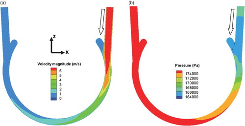
Figure 5(a) shows a strong acceleration at the inlet, and a maximal velocity of 6.14 m/s is reached near the inner wall. By the middle of the curved duct, near the tenth nozzle, the flow has separated from the outer wall and the separation zone grows downstream. A major feature is that the mean velocity decreases along the distributor due to the fluid discharge through the successive orifices. The pressure tends to increase from 1.65 × 10⁵ Pa to 1.75 × 10⁵ Pa along the curved channel (Figure 5(b)), showing that the Venturi effect overcomes the pressure drop.

Figure 7 shows flow streamlines and velocity contour lines in the curved duct cross-section relative to Nozzle 5. The flow structure inside the orifice is not affected by its diameter. Indeed, the jet is asymmetrical: high velocity is detected at the edge of the boundary layer, which undergoes a large deflection due to the Borda effect. An increase in the orifice diameter moves the vortex toward the outer wall. Qualitatively, the same flow pattern is also seen when varying the flow rate from 3.8 to 6 m³/h. In the flow-rate range, the outlet velocity is between 10 and 120 m/s for d = 0.8 mm, and decreases to 1 to 12 m/s for d = 2.5 mm and 0.5 to 4 m/s for the widest orifice, d = 4.2 mm.

Figure 6. Sections along the distributor.

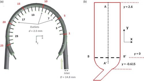
In order to examine the velocity pattern along the curved channel we defined several sections along the vertical and horizontal axes, designated respectively by AA′ and BB′. Section 1 corresponds to the vertical section (AA′) above the first orifice and so on. The six sections correspond to Orifices 1, 5, 10, 15, 20 and 25, respectively (Figure 7). It should be noted that the sections along AA′ are adjacent to the plane y = 0 and BB′ extends from the ordinate y = −0.65 cm to y = 2.6 cm.

Figure 7. Computed velocity field (m.s⁻¹) for nozzle diameters of (a) d = 0.8 mm, (b) d = 2.5 mm and (c) d = 4.2 mm in the streamwise cross-section of Nozzle 5.

Figure 8 compares typical numerical velocity profiles along AA′ for different geometric configurations. In all cases, the velocity increases in the vicinity of the jet zone. The orifice cross-section is very small compared to that of the distributor; high turbulence activity is seen in this zone. For the smallest orifice diameter, the velocity profile is more stable, and the influence of the secondary flow is not significant in this case. This is clearly seen for d = 0.8 mm (Figure 8(a)). Unlike the other profiles, here the velocity varies locally due to the effect of the secondary flow caused by the centrifugal force.

Figure 8. Numerical velocity magnitude along the distributor (axis AA′) for nozzle diameters (a) d = 0.8 mm, (b) d = 2.5 mm and (c) d = 4.2 mm for Q = 3.8 m³/h.

Other numerical velocity profiles along the channel width (BB′ axis) are plotted in Figure 9. For the inlet flow rate of Q = 3.8 m³/h, the velocity profiles show the same trend. Maximum values are close to the inner wall for Section 1 and close to the outer wall for Section 5, and much smaller velocity values are detected at the centerline. The highest magnitudes of the velocity component are observed closer to the inner wall in Section 1, and as the flow develops in the channel, the maximum value deflects toward the outer wall.

Figure 9. Numerical velocity magnitude along the distributor (axis BB′) for nozzle diameters (a) d = 0.8 mm, (b) d = 2.5 mm and (c) d = 4.2 mm for Q = 3.8 m³/h.

The estimated mean velocity distribution on the centerline of the curved channel is shown in Figure 10, together with the theoretical mean velocity. These values are taken for the different orifice diameters (d = 0.8, 2.5 and 4.2 mm) and the inlet flow rate of Q = 3.8 m³/h. For the different cases, the velocity tends to decrease as the flow moves downstream due to the flow discharge through the orifices spread along the distributor.

Figure 10. Computed and theoretical velocity magnitudes at the centerline for different nozzle diameters for Q = 3.8 m³/h.

Repetitions of the measurements indicate a standard deviation of 13% for the first two nozzles and the last one; this error is due to the undeveloped aspect of the flow at the beginning and the loss in kinetic energy when the fluid reaches the end. For nozzles located at the middle of the distributor, the error decreases to 4%.

3.1.3. Turbulence field

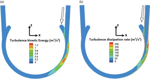
The computed TKE field and its dissipation rate (ε) in the axial cross section y = 1 are presented in Figure 11. In the curved region, TKE production is high (1.6 m²/s²). Moreover, the TKE dissipation rate ε increases in the curved zone and the turbulence tends to subside at the end of the channel.

Figure 11. Computed hydrodynamic fields for the axial cross section y = 1 for: (a) TKE contours (m²/s²); (b) TKE dissipation rate contour.

The computed normalized TKE at the centerline is provided in Figure 12 for the three orifice diameters (d = 0.8, 2.5 and 4.2 mm) and the same inlet flow rate (Q = 3.8 m³/h). The turbulence intensity I, reflected by the normalized term listed above, is estimated by (1) where U is the mean velocity. At the beginning of the duct, the turbulence level is arbitrary (Hinze hypothesis: 10%), and quickly the inlet turbulence relaxes and reaches its true balance downstream; its maximum value is attained near to the zone extended from Nozzle 5 to 10. The normalized profiles are similar for the three geometries.

Figure 12. Computed normalized TKE at the centerline for different nozzle diameters for Q = 3.8 m³/h.

3.2. Discussion

Here we examine the agreement among the numerical and experimental approaches on the global flow-rate–pressure relationship. These are compared with so-called ‘theoretical results’ based on the hydraulic balance, for which basic equations are given in section 3.2.2 below.

At first, in the following section, PIV and CFD results are briefly compared, then flow streamlines and several flow images for different cross-sections along the geometry are presented for the different geometry parameters listed in Table 3.

Table 3. Internal relative pressure for different nozzle diameters and inlet flow rates.

	Theoretical pressure (Pa)		Numerical pressure (Pa)		Experimental pressure (Pa)
Q (m^3/h)	3.8	6	3.8	6	3.8	6
d = 0.8 mm	3.53 × 10^6	8.79 × 10^6	4.30 × 10^6	10.80 × 10^6	-	-
d = 2.5 mm	3.70 × 10^4	9.22 × 10^4	3.83 × 10^4	9.32 × 10^4	2.35 × 10^4	7.9 × 10^4
d = 4.2 mm	4.60 × 10^3	1.16 × 10^4	2.60 × 10^3	-	-	-

3.2.1. PIV and CFD flow patterns

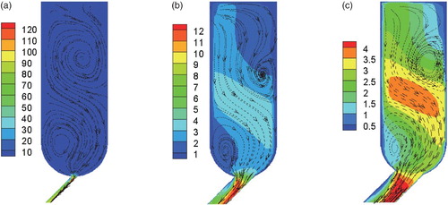
The different flow cross-sections in Figure 13 were taken respectively at the beginning (Orifice 5), middle (Orifice 13) and end (Orifice 20) of the distributor using the PIV technique. Some parts of the duct sections were masked in processing the PIV measurements due to light reflections and aberrant velocity vectors. This image processing caused a loss of 5–15% of the actual images. As a consequence of this filtering, three zones have been designated A, B and C for the purpose of comparison and to show the sense of rotation of the vortex (Figure 13).

Figure 13. Comparison between PIV experimental results and CFD simulations of the velocity field in a cross-section for Q = 3.8 m³/h and d = 2.5 mm.

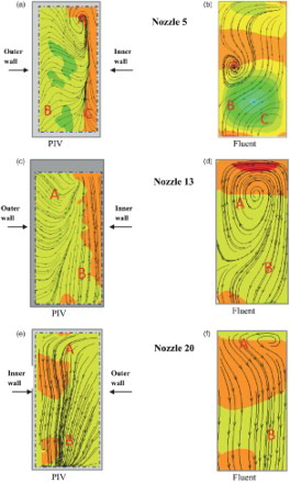
One can see the close similarities in the streamline patterns on the velocity profiles between the experimental and numerical results, despite the impossibility to check the local values pixel by pixel. Notice that the PIV is used only to get insights about the flow in the distributor. However, the experimental validation of our numerical model could not be achieved without experimental measurements of the pressure drop and flow rates along the different nozzles of the distributor. The results are presented in the following section.

3.2.2. Axial pressure profile

Pressure profiles along the distributor are plotted in Figure 14. Theoretical values are evaluated by a model reflecting the hydraulic balance. For each orifice, the discrete scheme of the equations below is resolved: (2) (3) with the integral condition , where V_i is the superficial velocity in the channel, v_i the superficial velocity in orifice I, p_i is the inner relative pressure on the channel axis and ξ is the Borda pressure drop coefficient at the orifice. This algebraic model gives the head pressure p₀ with an iterative procedure.

Figure 14. CFD compared to theoretical pressure profiles along the distributor for different nozzle diameters for Q = 3.8 m³/h.

For the inlet flow rate of Q = 3.8 m³/h, the orifice pressure distribution shows the highest relative pressure value of 3.7 × 10⁶ Pa for the smallest orifice cross-section (d = 0.8 mm). The trends of the theoretical and computed values are clearly similar, but even with a maximum pressure drop coefficient of 1, the theoretical model underestimates the head pressure. This could justify the use of the CFD model for accurate sizing; it appears that the curvature induces a significant overconsumption of energy in this Reynolds number range. A visible increase in the pressure profile is observed for the largest orifice diameter. This can be explained by the balance between the static and dynamic pressures given by Equation (2).

Figure 15 compares the CFD-computed relative pressure with the theoretical and experimental results for orifice diameter d = 2.5 mm and an inlet flow rate of Q = 3.8 m³/h. This figure shows that the pressure profiles follow the same trend for the different cases. The pressure increases at the beginning (Orifices 1 to 5), then stabilizes and remains constant up to the end of the channel. A small discrepancy is observed in the experimental results at the first and last orifices.

Figure 15. CFD compared to theoretical and experimental pressure profiles along the distributor for nozzle diameter d = 2.5 mm and Q = 3.8 m³/h.

The error bars represent the systematic characteristic of the measurement instrument together with the random experimentation error. The global error on the pressure is estimated to be 5.92%.

3.2.3. Orifice flow rate

Plots of computed and theoretical distributed flow rates at the orifice outlets are shown in Figure 16 for an inlet flow rate of Q = 3.8 m³/h. The injected flow rates of the first and last orifices are less than the others. At the first orifice, this is only due to a lower inner pressure, but at the end of the duct, the flow is disturbed by a wide recirculation. As a result, Orifice 25 is fed only weakly by the main flow. The injected flow increases from the first orifice to the fifth, where the high-pressure zone is located – after that, it stabilizes and an equal flow rate is observed until it reaches the last orifice. It should be noted that this behavior cannot be avoided, even by increasing the main flow rate.

Figure 16. CFD computed and theoretical distributed flow rates at outlets for different nozzle diameters, Q = 3.8 m³/h.

A detailed analysis of Figure 16 shows the same trend in injected flow behavior for the same inlet flow rate and different orifice diameters (d = 0.8, 2.5 and 4.2 mm). The flow is always uniformly distributed among the different orifices starting from the fifth, while it increases gradually between the first and fifth orifice. The flow rate increase along the channel appears to be more pronounced when the orifice diameter increases to 4.2 mm, which follows the relative pressure increase along the distributor; it is maximum for this large orifice diameter. The discrepancy between the numerical and theoretical flow rate values does not exceed 5%.

Figure 17 compares the theoretical, numerical and experimental results for the jet flow rates for the diameter d = 2.5 mm and an inlet flow rate of Q = 3.8 m³/h. Good agreement can be seen at the four orifices where the flow rates were measured. The same trend as at the beginning is detected: the first orifice up to the fifth show an increasing flow rate, then after the fifth orifice, the ejected flow rate becomes stable – and this is observed for the two inlet flow rates. The discrepancy observed in the last orifice flow rate is due to experimental error of about 10%. Subsequently, the numerical model is in good agreement with the experimental results.

Figure 17. CFD compared to theoretical and experimental distributed flow rates at outlets for nozzle diameter d = 2.5 mm and Q = 3.8 m³/h.

The global error on the experimental flow rate values, represented by the error bars in Figure 17, is estimated to be 4.5%.

3.2.4. Flow-rate–pressure relationship

The performance of the coolant distributor whose multiple orifices provide sprinkling jets on a cooling device can be assessed by establishing the flow-rate–pressure relationship at the inlet of the distributor. Figure 18(a) shows the variation in the inlet pressure as a function of the orifice diameter. The values presented here are theoretical, numerical and experimental, the latter for one orifice diameter (d = 2.5 mm) and an inlet flow rate of Q = 3.8 m³/h. Obviously, as the orifice diameter decreases, more pressure is required at the inlet; in other words, the coolant distributor consumes increasing energy but provides higher kinetic energy to the jets and an improvement on the heat removal.

Figure 18. (a) Distributor pressure as a function of nozzle diameter; (b) Flow-rate–pressure relationship for the distributor.

The variation in the head pressure as a function of inlet flow rate is presented in Figure 18(b). Theoretical, numerical and experimental values for the three orifice diameters are shown to follow a power-law with the exponent 2, as expected. Pressure increases with an increasing inlet flow rate and a decreasing orifice diameter. Theoretical, numerical and experimental pressure values are compared in Table 3. Good agreement is seen between the numerical and experimental curves, but both are seen to be twice the theoretical values, suggesting that the theoretical model does not completely capture the underlying physics of the flow. The relative error between the theoretical and experimental values increases from 14% to 35% as the inlet flow rate decreases from 6 m³/h to 3.8 m³/h.

3.2.5. Jets: a quick overview

The jets emanating from the orifices are in the turbulence regime, as the computed jet Reynolds numbers (Re_j) are greater than 3000 (values of Re_j are given in Table 4). Based on previous studies (Cushman-Roisin, 2010), the length of the potential core of a planar jet was estimated at about 4 to 7.7d, where d is the orifice diameter. In the present case, the ratio between the workpiece distance (H) and the orifice diameter is between 1.4 and 7.5, implying that the cooling zone (wheel-workpiece contact point) is located in the jet potential core region where the velocity conserves up to 99% of its initial value. A more detailed study of the interaction between the workpiece and the jets is planned.

Table 4. Computed jet Reynolds number for different nozzle diameters and inlet flow rates.

	Rej		H/d
Q(m^3/h)	3.8	6
d = 0.8 mm	68,720	108,632	7.5
d = 2.5 mm	22,175	35,075	2.4
d = 4.2 mm	13,440	–	1.4

3.2.6. Remediation for the end-recirculation

Optimizing distributor coolant geometry in industrial applications is of prime importance for better productivity as well as for cost savings. In order to remedy the recirculation vortex at the end of the distributor, a case in which the outlet sections were opened wide for the evacuation of the water towards the outside was simulated. Two peripheral circular sections of diameter 6.15 mm (A and B in Figure 1(a)) were opened at the extremities of the distributor. This modification caused a natural decrease in the cooling flow rates at the orifices, since a large amount of the water was directly evacuated through the openings. In addition, recirculation persisted at the extremities of the distributor. Also, extending the outlet with a longer downstream tube did not seem to produce better results: fluid acceleration in the case of open outlets and wall impact in the closed-extremity configuration caused flow stirring and recirculation, producing additional head losses. As a conclusion, it is not easy to fix the last orifice defect, but the whole system ought to be efficient enough.

4. Conclusion

A study using CFD simulations and experimental investigation into the complex turbulent flow through a curved channel equipped with multiple discharge orifices delivering the coolant fluid in grinding processes was performed in order to identify the main geometrical features for such water-jet distributors.

For a given inlet flow rate and orifice diameter, the flow rates are not uniformly distributed at the orifices, and the distribution depends on the inner pressure field that arises out of the complex flow pattern: the main effects were identified to be the recirculations, the TKE dissipation (pressure drop), and the Venturi effect due to the flow rate drop along the distributor. A global flow-rate–pressure relationship was established for this special curved duct flow that allows extrapolation for any orifice diameter and flow rate.

Experiments and simulations are shown to be in a fair agreement, so that the tool for sizing and optimization is now effective for future industrial design, especially when coupling the heat removal study with the impinging jets on the grinding wheel/workpiece interface.

Disclosure statement

No potential conflict of interest was reported by the authors.

References

- ANSYS (2006). Fluent 6.3 User's Guide.
- Aziz, T. N., Raiford, J. P., & Khan, A. A. (2008). Numerical simulation of turbulent jets. Engineering Applications of Computational Fluid Mechanics, 2(2), 234–243. doi: 10.1080/19942060.2008.11015224
- Cushman-Roisin, B. (2010). Turbulent Jets. Thayer School of Engineering at Dartmouth. Daramouth College, 032010. Retrieved from http://thayer.darmouth.edu/cushman/books/EFM/chap9.pdf
- Davis, P. L., Rinehimer, A. T., & Uddin, M. (2012). A comparison of RANS-based turbulence modeling for flow over a wall mounted square cylinder. N C Motorsports and Automotive Research Center Department of Mechanical Engineering and Engineering Science, The University of North Carolina at Charlotte, Charlotte, NC 28223, USA.
- Goldstein, R. J., & Seol, W. S. (1991). Heat transfer to a row of impinging circular air jets including the effect of entrainment. International Journal of Heat and Mass Transfer, 34, 2133–2147. doi: 10.1016/0017-9310(91)90223-2
- Hidayat, M., & Rasmuson, A. (2004). Numerical assessment of gas-solid flow in a U-bend. Chemical Engineering Research and Design, 82(A3), 332–343. doi: 10.1205/026387604322870444
- Hinze, O. (1975). Turbulence (2nd ed.). New York, NY: McGraw-Hill.
- Iacovides, H., Launder, B. E., & Li, H.-Y. (1996a). Application of a reflection-free DSM to turbulent flow and heat transfer in a square-sectioned U-bend. Experimental Thermal and Fluid Science, 133, 419–429. doi: 10.1016/S0894-1777(96)00096-9
- Iacovides, H., Launder, B. E., & Li, H.-Y. (1996b). The computation of flow development through stationary and rotating U-ducts of strong curvature. International Journal of Heat and Fluid Flow, 17, 22–33. doi: 10.1016/0142-727X(95)00056-V
- Jaramilloa, J. E., Pérez-Segarraa, C. D., Rodrigueza, I., & Olivaa, A. (2008). Numerical study of plane and round impinging jets using RANS models. Numerical Heat Transfer, Part B: Fundamentals, 54(3), 213–237. doi: 10.1080/10407790802289938
- Kim, J., Yadav, M., & Kim, S. (2014). Characteristics of secondary flow induced by 90 degree elbow in turbulent pipe flow. Engineering Applications of Computational Fluid Mechanics, 8(2), 229–239. doi: 10.1080/19942060.2014.11015509
- Launder, B. E., & Spalding, D. B. (1972). Lectures in mathematical models of turbulence. London: Academic Press.
- Lytle, D., & Webb, B. W. (1994). Air jet impingement heat transfer at low nozzle-plate spacings. International Journal of Heat and Mass Transfer, 37, 1687–1697. doi: 10.1016/0017-9310(94)90059-0
- Momayez, L., Dupont, P., Delacourt, G., Lottin, O., & Peerhossaini, H. (2009). Genetic algorithm based correlations for heat transfer calculation on concave surfaces. Applied Thermal Engineering, 29, 3476–3481. doi: 10.1016/j.applthermaleng.2009.05.025
- Momayez, L., Dupont, P., Delacourt, G., & Peerhossaini, H. (2010). Eddy heat transfer by secondary Görtler instability. Journal of Fluids Engineering- Transactions of the ASME, 132(4), Paper 041201–041201-10. doi: 10.1115/1.4001307
- Momayez, L., Dupont, P., & Peerhossaini, H. (2004a). Effects of vortex organization on heat transfer by Görtler instability. International Journal of Thermal Sciences, 43, 753–760. doi: 10.1016/j.ijthermalsci.2004.02.015
- Momayez, L., Dupont, P., & Peerhossaini, H. (2004b). Some unexpected effects of wavelength and perturbation strength on heat transfer enhancement by Görtler instability. International Journal of Heat and Mass Transfer, 47, 3783–3795. doi: 10.1016/j.ijheatmasstransfer.2004.04.006
- Moussa, T., Garnier, B., & Peerhossaini, H. (2013). Measurement and modeling of thermal properties of sintered diamond composites for grinding applications. Journal of Alloys and Compounds, 551, 636–642. doi: 10.1016/j.jallcom.2012.11.025
- Moussa, T., Garnier, B., & Peerhossaini, H. (2015a, May). Nouvelle méthode de mesure de la température de paroi du verre au cours de son meulage et effet des paramètres de façonnage [Novel method for glass surface temperature measurement during grinding and the influence of grinding parameters]. Paper presented at the Congrès Annuel de la Société Francaise de Thermique, La Rochelle, France.
- Moussa, T., Garnier, B., & Peerhossaini, H. (2015b, May). Résistance thermique de contact et flux généré à l'interface meule diamantée / verre au cours de son processus de meulage [Thermal contact resistance and generated heat flux at the wheel / glass interface during grinding]. Paper presented at the Congrès Annuel de la Société Francaise de Thermique, La Rochelle, France.
- Ockfen A. E., & Matveev K. I., (2009). Numerical modeling of a planar unconfined oblique jet moving along the ground surface. Engineering Applications of Computational Fluid Mechanics, 3(2), 242–257. doi: 10.1080/19942060.2009.11015268
- Peerhossaini, H., & Bahri, F. (1998). On the spectral distribution of the modes in nonlinear Görtler instability. Experimental Thermal and Fluid Science, 16, 195–208. doi: 10.1016/S0894-1777(97)10029-2
- Prasad, A. K. (2000). Particle image velocimetry. Current Science, 79(1), 51–60.
- Wei, J., Zhang, J., Li, S., & Wang, F. (2015). Numerical study on impinging-film hybrid cooling effect with different geometries. International Journal of Thermal Sciences, 92, 199–216. doi: 10.1016/j.ijthermalsci.2015.01.038
- Womac, D. J., Ramadhyani, S., & Incropera, F. P. (1993). Correlating equation for impingement cooling of small heat sources with single circular liquid jets. Journal of Heat and Mass Transfer, 115, 106–114.