Assessment of particle-tracking models for dispersed particle-laden flows implemented in OpenFOAM and ANSYS FLUENT

ABSTRACT

In the present study two benchmark problems for turbulent dispersed particle-laden flow are investigated with computational fluid dynamics (CFD). How the CFD programs OpenFOAM and ANSYS FLUENT model these flows is tested and compared. The numerical results obtained with Lagrangian–Eulerian (LE) point-particle (PP) models for Reynolds-averaged Navier–Stokes (RANS) simulations of the fluid flow in steady state and transient modes are compared with the experimental data available in the literature. The effect of the dispersion model on the particle motion is investigated in particular, as well as the order of coupling between the continuous carrier phase and the dispersed phase. First, a backward-facing step (BFS) case is validated. As a second case, the confined bluff body (CBB) is used. The simulated fluid flows correspond well with the experimental data for both test cases. The results for the dispersed solid phase reveal a good accordance between the simulation results and the experiments. It seems that particle dispersion is slightly under-predicted when ANSYS FLUENT is used, whereas the applied solver in OpenFOAM overestimates the dispersion somewhat. Only minor differences between the coupling schemes are detected due to the low volume fractions and mass loadings that are investigated. In the BFS test case the importance of the spatial dimension of the numerical model is demonstrated. Even if it is reasonable to assume a two-dimensional fluid flow structure, it is crucial to simulate the turbulent particle-laden flow with a three-dimensional model since the turbulent dispersion of the particles is three-dimensional.

KEYWORDS:

• CFD
• Lagrangian-Eulerian approach
• backward-facing step
• confined bluff body
• stochastic dispersion model

1. Introduction

Dispersed particle-laden flows are found in many technical applications, e.g., pneumatic conveying, particle separation and fluidized beds (Sommerfeld, von Wachem, & Oliemans, 2008). In order to design, optimize or upscale such processes and their corresponding machines, a detailed prediction of those complex fluid flows by means of numerical simulation is of great interest to engineers. Computational fluid dynamics (CFD) offers the possibility of gaining an insight into a wide range of fluid flows. In recent years CFD models have been developed which depict particle–fluid and also particle–particle interaction in laminar or turbulent flows with increasing accuracy. A detailed and comprehensive review of this field of research is beyond the scope of the current paper; therefore, the reader is directed to the following interesting and relevant textbooks (Clift, Grace, & Weber, 2005; Crowe, Sommerfeld, & Tsuji, 1998) and reviews (Balachandar & Eaton, 2010; Deen, Van Sint Annaland, Van der Hoef, & Kuipers, 2007; Subramaniam, 2013; Zhou, Kuang, Chu, & Yu, 2010; Zhu, Zhou, Yang, & Yu, 2007).

The order of coupling between the dispersed and continuous phase is initially determined by the volume fraction of the solid material, . In Figure 1 the classification map proposed by Elghobashi (1994) is shown. According to this map, a one-way coupling can be used for highly diluted flows with . The flow of the carrier fluid influences the particle trajectories, but the particles have a negligible effect on the flow turbulence. For volume fractions of particles affect the turbulence in the flow. A two-way coupling between the phases must be used in order to account for the additional feedback force exerted on the flow by the particles. The degree of influence depends on the ratio of the particle reaction time, , to the Kolmogorov time scale, , respectively the turnover time of large eddies, , where and are the density and diameter of the particles is the fluid density, is the kinematic viscosity, is the turbulence dissipation rate, is the turbulent length scale and is the velocity magnitude. Small values of increase turbulence dissipation while large particle reaction times enhance turbulence production. As the volume fraction exceeds , additional particle–particle interactions occur which are referred to as four-way coupling. Besides the volume fraction the mass loading must also be considered here, as described in Kulick, Fessler, and Eaton (1994) and Vreman (2015). A high particle mass loading increases the attenuation of the flow turbulence.

Figure 1. Classification of coupling schemes and interaction between particles and turbulence according to Elghobashi (1994) for (1) one-way coupling, (2) two-way coupling where particles enhance turbulence production, (3) two-way coupling where particles enhance turbulence dissipation, and (4) four-way coupling.

To describe multiphase flows, the Lagrangian–Eulerian (LE) approach can be used. In contrast to other approaches it can handle a wide range of particle sizes in both diluted and dense flows and captures nonlinear, multiscale interactions as well as non-equilibrium effects (Subramaniam, 2013). In doing so, the Navier–Stokes equations are solved for the continuous carrier phase. The dispersed particle phase is resolved by tracking particles through the gas flow. Both phases exchange momentum to allow an interaction. It is common to idealize large numbers of particles as ‘point-particles’ (PP). Particle boundary layers, wake flow regions and similar flow processes on particle or sub-particle scales are not resolved. These effects are modeled via functional correlations with empirical parameters. Options for the PP approach are characterized by the solution of the continuous phase, which can be accomplished on the basis of Reynolds-averaged Navier-Stokes (RANS) equations, large eddy simulation (LES) where large-scale turbulence is resolved or direct numerical simulations (DNS). For PP-LES and PP-RANS the particle size has to be much lower than the grid-cell size.

For basic research, PP-LES or even PP-DNS are often employed to study mechanisms in detail. Recent examples of particle-laden channel and confined bluff body (CBB) flow can be found in, for example, Breuer and Alletto (2012), Mallouppas and van Wachem (2013), Sardina, Schlatter, Brandt, Picano, and Casciola (2012) and Wang, Manhart, and Zhang (2011), while turbulence modification in turbulent particle-laden channel flows can be found in Vreman (2015). CFD simulations for basic research are often performed with in-house CFD programs like LESOCC (Breuer & Alletto, 2012) and numerical data is routinely validated in detail via the comparison of calculated and measured basic flow data, e.g., velocities or root mean square (RMS) values of turbulent fluctuations.

For applied research, particle-laden flows at the industrial scale are typically studied in the context of PP-RANS (Portela & Oliemans, 2006). Some recent examples of PP-RANS studies using in-house CFD programs include Laín and Sommerfeld (2012) for particle-laden flows with high mass loading in pneumatic conveying and Corsini et al. (2014) for particle-laden flows in axial and centrifugal fans.

In contrast, CFD simulations for engineering applications are typically performed with well-established CFD packages such as ANSYS FLUENT, ANSYS CFX, STAR CCM+ and OpenFOAM (for recent examples, see Burlutskiy & Turangan, 2015; Kim, Ng, Mentzer, & Mannan, 2012; Lin, Lan, Xu, Dong, & Barber, 2015; Saffari & Hosseinnia, 2009; Torti, Sibilla, & Raboni, 2013; Weber, Schaffel-Mancini, Mancini, & Kupka, 2013). In these studies, the performance of the numerical model is often tested via the comparison of numerical and experimental process parameters, e.g., pressure losses in pipe flows or species concentration. A critical evaluation of the basic flow and dispersed phase data is often missing. It must be assumed that there is basic confidence in the reliability of the CFD software, although the agreement between numerical and experimental findings is sometimes poor.

The goal of the present study is therefore a fundamental validation of the PP-RANS models in actual versions of two well-known CFD packages, ANSYS FLUENT and OpenFOAM. A short description of the PP-RANS model fundamentals in both software packages is given, after which the PP-RANS models are tested for one- and two-way coupling. Two well-documented experiments – the particle-laden flow over a backward facing step (BFS; Fessler & Eaton, 1999) and the particle-laden flow in a confined bluff body (CBB, Borée, Ishima, & Flour, 2001) – serve as benchmark problems. To begin with, the CFD simulations were performed with the recommended (standard) model parameters, after which the model parameters were modified in order to test whether or not the differences between the numerical and experimental data could be reduced.

2. Numerical modelling

2.1. Basic Lagrangian–Eulerian model

In order to investigate dispersed flow of inert particles, the LE frame of the conservation equations is used. For the isothermal, incompressible, turbulent flow of a Newtonian fluid, which is the continuous carrier phase, the mass and momentum transport in the fluid phase are described by the RANS equations as follows: (1) (2) where and are the Reynolds-averaged flow velocity and pressure, is the fluid density, is the dynamic viscosity and is the additional body forces. The Reynolds stresses, , are typically modeled using an eddy-viscosity approach. In the present study, two turbulence models are used in combination with wall functions, namely the standard model (Launder & Spalding, 1974) and the -SST model (Menter, 1994). Both models are based on the eddy viscosity approach and contain two equations for the turbulent kinetic energy and the turbulent dissipation , respectively, along with the turbulent specific dissipation rate . Information about the specific implementations in ANSYS FLUENT and OpenFOAM can be found in the user guides (ANSYS FLUENT, 2014; OpenFOAM, 2014).

For the dispersed phase, the particle motion is solved by integrating the force balance, which is written in a Lagrangian frame on the particles. In the set of differential equations that calculate particle locations and velocities, it is assumed that the particles are spherical, while heat and mass transfer are neglected. Furthermore, all particles are treated as point masses by the CFD code so that an equation for the torque is omitted: (3) (4) where is the position vector of the particle, is the particle velocity and is the particle mass. The term represents the sum of all relevant forces, (5) where is the drag force, is the buoyancy force and is the gravitational force. These terms contain the major influences on the particle trajectory, while other forces, such as the Basset history term, are neglected.

The drag force is implemented in both CFD programs as follows: (6) where is the particle diameter and the drag coefficient is reliant on the flow regime. According to Crowe et al. (1998) can be calculated via a non-linear function in the dependency of the particle Reynolds number : (7)

In contrast to the suggested approach, OpenFOAM uses the following slightly modified empirical relation when spheres are considered: (8)

By choosing the spherical drag law in ANSYS FLUENT, is taken from: (9)

As stated in the ANSYS FLUENT Theory Guide (2014), the constants , and given by Morsi and Alexander (1972) apply over several ranges of Reynolds numbers. The same relation for as in OpenFOAM (Equation (8)) is applied when the dynamic drag model theory is selected. ANSYS FLUENT suggests this model for spray modeling when variations in the droplet shape have to be taken into account. However, no substantial influence on the particle motion was detected, as different drag models were used.

The buoyancy and gravitational force are calculated as follows in both CFD programs: (10)

2.2. Coupling of dispersed and continuous phases

For simulating particle-laden flows, an appropriate coupling of dispersed and continuous phases must be defined. The decision about the coupling scheme is reliant on the volume fraction of the particles, as shown in the classification map in Figure 1 (Balachandar, 2009; Elghobashi, 1994). The particle motion in diluted flows is primarily influenced by the aerodynamic forces acting on the particles. Since particle–particle interactions and the effect of the dispersed phase on the fluid flow are negligible, a one-way coupling is sufficient. In this case, no additional body forces appear in the momentum equation (Equation (2)) of the fluid phase, i.e., .

If the volume fraction of the dispersed phase increases, the influence of the dispersed phase on the fluid flow has to be taken into account. By enabling a two-way coupling, such a momentum exchange is realized with in Equation (2). Source terms, which will be transferred in the time step to the continuous phase momentum equation, are formulated with a dependency on the particle mass flow rate , the time step and the forces on the particles.

Furthermore, if interactions between particles have to be considered at high volume loadings, a four-way coupling must be enabled, at which point particle collisions are resolved within the Lagrange solver. However, such effects are not investigated in the present study.

2.3. Particle dispersion

The integration of particle trajectories from Equations (4) to (7) requires information of the instantaneous fluid velocity , which is not provided by the solution to the RANS equations (Equations (1) and (2)) of the fluid flow. Therefore the fluctuating velocity has to be estimated in order to model the turbulent dispersion of the particles by either stochastic or deterministic methods.

Here the stochastic eddy lifetime method, also referred to as a discrete random walk (DRW) model, is applied. In doing so, the generation of a fluctuating velocity part is realized by using a Gaussian distribution function. The characteristic eddy lifetime determines the range over which the random value of the fluctuating components is kept constant (Sommerfeld, 1995). On the assumption of isotropic turbulence, the standard deviation can be described through: (11)

The implementation of this method in ANSYS FLUENT (2014) is a follows: (12) where is a vector formed by normally distributed random numbers. In OpenFOAM, an additional random vector is used for the calculation of to depict the spatial randomness of turbulence: (13) with the turbulent kinetic energy provided by the turbulence model.

3. Solver description

Care has been taken to use numerical methods, schemes and boundary conditions that are as similar as possible in both CFD codes (ANSYS FLUENT 14.5 and OpenFOAM 2.1.x) in order to ensure the comparability of the simulation results. Table 1 summarizes the main settings in the two investigated programs. It should be emphasized that it is not possible to have the exactly same settings, since the formulation of the models in the CFD codes are different. For the model setup in ANSYS FLUENT, primarily the recommended default settings are applied, as would be done by a standard user. The settings in OpenFOAM are selected using the benefit of the long-term experience of the authors.

Table 1. Numerical methods, schemes and boundary conditions in ANSYS FLUENT and OpenFOAM.

	ANSYS FLUENT	OpenFOAM
Numerical methods steady
Solver	Pressure-based	simpleFoam
Pressure–velocity coupling	SIMPLE	SIMPLE
Multigrid	AMG	GAMG
Under-relaxation factors	0.3 – pressure	0.3 – pressure
	0.7 – momentum	0.7 – momentum
	0.8 – turbulence	0.7 – turbulence
Numerical methods transient
Solver	Pressure-based	pimpleFoam
Pressure–velocity coupling	SIMPLE	PIMPLE
Spatial discretization
Pressure	Standard	linearUpwind
Convective terms	Second-order upwind	linearUpwind
Gradient	Green–Gauss node-based	Gauss linear

3.1. Fluid phase

In both programs, pressure-based solvers are used for the solution of the carrier fluid flow. The pressure–velocity coupling is accomplished with the SIMPLE algorithm (Patankar & Spalding, 1972). In ANSYS FLUENT, the second-order upwind scheme is applied for interpolation in all model equations. The pressure is discretized with the Standard scheme and the gradients with the Green–Gauss node-based gradient evaluation. The resulting system of discretized equations is solved with the algebraic multigrid (AMG) method using a point-implicit linear equation solver (Gauss–Seidel). The under-relaxation factors correspond to the default settings in ANSYS FLUENT (Table 1).

In OpenFOAM, the solver simpleFoam (OpenCFD, 2014) is utilized for the solution of the fluid flow. In all model equations linear upwind scheme is used for interpolation and linear scheme for discretization of gradients. The discretized equations are solved with the geometric algebraic multigrid (GAMG) method in conjunction with the Gauss–Seidel solver.

3.2. Dispersed phase

On the basis of the generated background fluid flow field, the solvers release a defined number of particles at an absolute position in the flow domain which are then tracked as they travel through the flow domain.

For one-way coupling between the continuous fluid and the dispersed particle phase, the particles were tracked passively through the fluid phase, i.e., without their having any effect on the fluid flow. In OpenFOAM the pimpleLPTbubbleFoam solver with deactivated phase coupling was used for this purpose, which was developed by van Vliet et al. (2013) and is equivalent to the solver DPMFoam that is included in OpenFOAM 2.2.2 with little modification on the calculation of the body forces. In ANSYS FLUENT, one-way coupling was realized with the discrete phase model with ‘interaction with the continuous phase’ not selected.

For two-way coupling between the phases, the impact of the particle phase on the fluid flow must be taken into account. In OpenFOAM, the same solver (pimpleLPTbubbleFoam) was used but with the coupling scheme activated. Both phases were solved sequentially at each time step and an explicit delivery of the source terms to the continuous phase was set. ANSYS FLUENT supports two-way coupling when the option ‘interaction with the continuous phase’ is selected and the recommended automated particle-tracking scheme was retained.

4. Backward-facing step (BFS)

4.1. Case description

The BFS is a canonical case for validation purposes regarding turbulent flows with separation and reattachment processes (Armaly, Durst, Pereira, & Schönung, 1983). It is also used as a benchmark problem for dispersed turbulent two-phase flows. Several experimental and numerical studies of particle-laden flows over the BFS can be found in the literature (Anwar-ul-Haque, Yamada, & Chaudhry, 2007; Fessler & Eaton, 1999; Hardalupas, Taylor, & Whitelaw, 1992; Hishida & Maeda, 1991; Kulick et al., 1994; Maeda, Kiyota, & Hishida, 1982; Mohanarangam & Tu, 2007; Thangam & Speziale, 1992).

From the available data, the experimental results of Fessler and Eaton (1999) are used as a benchmark in this study. The geometry for the simulation is described in Table 2 and Figure 2. Due to the high ratio of , it is reasonable to assume a two-dimensional fluid flow structure of the mean flow , . In the experiments the air flow at the inlet is turbulent and fully developed, which is ensured by the long channel flow development section (Fessler & Eaton, 1999). The particles come to equilibrium in the channel flow before they enter the test section.

Figure 2. Geometry of the BFS according to Fessler and Eaton (1999).

Table 2. Flow properties for the BFS.

Channel flow		BFS flow
Channel height		Step height
Channel width		w/H	17:1
h/H	5:3

Source: Fessler and Eaton (1999).

To investigate the influence of the grid dimension on the simulation of the particle-laden gas flow, four different meshes were used. A summary of all the grids and their properties is given in Table 3. For the 3D meshes, the channel width was always 0.1 m. ANSYS FLUENT accepts both two- and three-dimensional problems. Meshes A, C and D are utilized in this program. OpenFOAM only operates in a three-dimensional Cartesian coordinate system but can solve in two dimensions by designating the ‘empty’ boundary condition to the boundaries at the front and back; therefore, the meshes B, C and D were applied.

Table 3. Applied meshes.

Name	Dimension	Cells in z direction	Boundary condition front and back
Mesh A	2D	0	–
Mesh B	3D	1	Empty
Mesh C	3D	1	Symmetry
Mesh D	3D	10	Symmetry

The structured meshes for the numerical simulation were generated with the commercial tool ANSYS ICEM CFD. They contain 32,000 cells in the x-y plane with equidistant intervals along the main flow direction and a relative refinement along the step contour. Preliminary examinations showed that the refinement should be limited to a certain cell size because otherwise the solution might get unstable. To maintain the developed turbulent flow conditions, an inlet channel of about and a downstream channel of about in length are used.

4.2. Numerical setup

At the inlet patch, which is located at upstream of the step, a turbulent profile with an area-averaged mean velocity and a maximum velocity at is given. The air viscosity is . The Reynolds number of the flow is . A summary of the applied boundary conditions can be found in Table 4. For the simulation of the BFS flow, the -SST model was used (Anwar-ul-Haque et al., 2007).

The settings for the dispersed phase are shown in Table 4. Copper particles with a mass-averaged diameter of and a density of are inserted through a patch injection at the inlet. The particles are injected with a mass flow rate of and a velocity of for a duration of . The settings in ANSYS FLUENT and OpenFOAM for the trajectories to be calculated are matched to each other so that there are the same numbers of particles with equivalent mass loadings.

Table 4. Boundary and initial conditions for the BFS case.

Continuous phase
Inlet	Profile with
Outlet
Wall
Dispersed phase
Particle diameter
Particle density
Particle mass flow rate
Injection velocity

The mass loading and volume fraction of solid material () is low for the simulated particle-laden BFS flow. However, it is resolved in both one- and two-way coupled numerical simulations. For one-way coupling, first the RANS simulation of the continuous phase and the DPM modeling of the dispersed phase are executed sequentially. For two-way coupling, the URANS simulation of the continuous phase and the DPM modeling of the dispersed phase run together. In this case, the steady-state flow field data are used as initial values for the URANS simulations, then the Courant number is set to a value of 0.3. In the corresponding ANSYS FLUENT case setup, a fixed time step is used.

4.3. Results

4.3.1. Continuous phase

Figure 3 presents the development of normalized flow profiles along the channel. They are somewhat amplified in order to highlight deviations. The solution of the fluid flow is independent from the mesh dimension.

Figure 3. Comparison of the flow profiles of the continuous phase behind the BFS from simulations in ANSYS FLUENT and OpenFOAM and experiments according to Fessler and Eaton (1999), for the velocity distribution of the main component (top), and distribution of the velocity fluctuation (bottom).

Note: The baseline locations of the profiles are at .

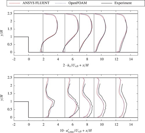
Looking at the top diagram in Figure 3, the typical flow profiles of can be recognized. Directly behind the step a recirculation zone arises where backflow occurs. The reattachment of the flow happens at approximately . All in all a close resemblance between the simulations and the experiment can be seen. Only slight deviations of occur in the region between the recirculation and the main flow. Focusing on the flow further downstream, the plot shows that the velocities at the lower wall are underestimated by the simulation by . By just considering the numerical results, hardly any difference between ANSYS FLUENT and OpenFOAM can be found. The minimal deviations can be attributed to the different formulations of the wall functions.

In the bottom diagram in Figure 3, the experimentally and numerically determined velocity fluctuations in the main flow direction, , can be compared regarding the magnitudes and shapes of the profiles. Strong fluctuations appear behind the step in the shear layer between the recirculation zone and the upper channel flow. This region expands with increasing distance to the step and the profile becomes more uniform. The plot again shows a good qualitative agreement between the profiles from both CFD programs and the experiment. However, a noticeable difference in amplitude between the numerical and experimental data is also visible.

4.3.2. Dispersed phase

In order to validate the dispersed phase, the profiles of the particle velocities are plotted in a similar manner to those of the continuous phase. To generate these plots according to the experiments, particles are evaluated in slices around a baseline – thereby the slice thicknesses correspond to , with the center lying exactly at the measurement points. The diagrams show the experimental data as well as the numerical data with both one- and two-way coupling after an injection duration of . The profiles indicate the particle velocity (in the x direction) and also the spreading of the particle cloud (in the y direction). The results for the two-dimensional meshes A and B as well as mesh C are shown in Figure 4 and those for the three-dimensional mesh D are shown in Figure 5.

Figure 4. Comparison of the velocity profiles of the dispersed phase in the main direction behind the BFS from simulations in ANSYS FLUENT and OpenFOAM on meshes A, B and C and experiments according to Fessler and Eaton (1999).

Note: The baseline locations of the profiles are at .

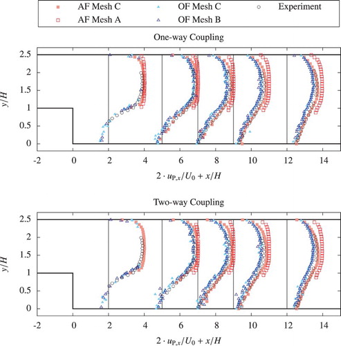
Figure 5. Comparison of the velocity profiles of the dispersed phase in the main direction behind the BFS from simulations in ANSYS FLUENT and OpenFOAM on mesh D and experiments according to Fessler and Eaton (1999).

Note: The baseline locations of the profiles are at .

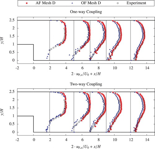
The data set from the experiment reveals that the particles mainly follow the fluid flow. Magnitude and shape are similar to the fluid flow profiles. Directly behind the step within the recirculation region no data are available since just a few particles were found there (Fessler & Eaton, 1999).

Turning to the simulation results in Figure 4, differences to the experiment can be found depending on the spatial dimension of the problem. The data set from the two-dimensional case in ANSYS FLUENT (mesh A) show velocities with a block profile distribution, which is not realistic. Contrary to the experiments, the particle cloud does not spread span-wise to the flow. No particle dispersion into the recirculation zone occurs. Furthermore the particle velocities are too high in all the profiles. For the two-way coupling in the bottom diagram no particles are detected at for the chosen time step since they have already passed this position. Apart from this observation, no influence regarding the coupling scheme can be observed at all for this case. The dispersed phase seems to be treated similarly in both one- and two-way coupling since it has no impact on the fluid flow. Several modifications of simulation settings do not lead to more physical results. Varying the particle time step, fluid flow time step, particle reaction time and mass loading only resulted in minor effects on the particle motion.

The results from the simulations with ANSYS FLUENT on mesh C, which has one cell layer in the span-wise (z) direction, match well with the experiment. Both the profile shape and velocity values are in good agreement. The simulated particle velocities are somewhat higher in the first four positions and the profiles are more block-shaped. However, at the position the curves for mesh C and the experiment overlay. Compared to the data from Fessler and Eaton (1999), the two-way coupled simulation with ANSYS FLUENT especially underestimates the expansion of the particle cloud behind the step at along the channel height. With the one-way coupling, the particles are already spread over the whole channel height at the second measuring point.

When including the ANSYS FLUENT results of the three-dimensional test case in the evaluation (Figure 5), only minor differences between mesh C and mesh D are found. For mesh D the shape of the profile at is closer to the experiment, but at the positions the spreading of the particle cloud along the channel height is still stronger with the one-way coupling.

From the data in Figures 4 and 5 it is apparent that the computational domain of ANSYS FLUENT simulations has to be three-dimensional when turbulent particle-laden flow is simulated, even if it is reasonable to assume a two-dimensional fluid flow structure – otherwise the three-dimensional character of turbulent dispersion gets lost and the spreading of the particle cloud is strongly underrated. These findings may also suggest that there is a bug in the two-dimensional dispersion model of ANSYS FLUENT.

Regarding the results from the OpenFOAM simulations in Figures 4 and 5, almost no difference between the order of coupling and the mesh can be observed. It seems to be irrelevant whether the ‘empty’ (mesh B) or ‘symmetrical’ (mesh C) boundary condition is used for the patches at the front and back. The velocity profiles of all the simulations are in good accordance with the experimental data, especially on the second measuring point in the area with dominating main flow as well as the region below the step. Here the deviations do not exceed . Looking at the particle distribution along the channel height, the simulations with OpenFOAM overestimate the turbulent dispersion compared to the experiment. However, the discrepancy between the experimental and numerical data grows with increasing distance to the step, and the velocity of the particles is underestimated in comparison to the experiment.

The slight differences between measured and numerical data might be caused by deviations in the setting of the boundary conditions. For instance, the effect of wall roughness on the particle-laden flow is neglected since the wall flow is not resolved. Particle data in particular in the wall-bounded flows is greatly influenced by wall roughness (Vreman, 2015). An error analysis for the experiment can be found in Fessler and Eaton (1999).

5. Confined bluff body (CBB)

5.1. Case description

The CBB flow is often used for model validation purposes where mixing and combustion of powdered materials are simulated (Alletto & Breuer, 2012; Apte, Mahesh, Moin, & Oefelein, 2003; Chrigui, Hidouri, Sadiki, & Janicka, 2013; Minier, Peirano, & Chibbaro, 2004; Oefelein, Sankaran, & Drozda, 2007; Sommerfeld & Qiu, 1993). Several of these studies compared their results with the experimental data from Borée et al. (2001), which is also used as benchmark in the present work.

Figure 6 gives a sketch of the CBB flow with the relevant geometric parameters. A particle-laden central jet () and an outer particle-free annular jet () are separated by a bluff body. The resulting flow structure consists of two stagnation points, S₁ and S₂, and a contra-rotating torus-shaped vortex pair, R₁ and R₂, which separates the central and annular jets between the inflow and the stagnation point S₂. Downstream from the stagnation point S₂, where the shear layers of the central and annular jets come into contact, a wake-like region similar to other bluff body flows is observed in Borée et al. (2001).

Figure 6. Geometry of the CBB test case according to Borée et al. (2001).

In this study the isothermal, incompressible CBB flow is resolved in a three-dimensional computational domain similar to the sketched region of Figure 6. The diameter of the central jet inflow is . The computational domain is discretized by 2.01 million hexahedral cells. In the region of the core flow the mesh is refined.

5.2. Numerical setup

Turbulent velocity profiles are used as initial boundary conditions for the air flow. At the jet inlet the area-averaged mean velocity is and the maximum velocity in the main flow direction in the center is . At the annular duct inlet an area-averaged velocity of is given. At the outlet the pressure is fixed and corresponds to the operating pressure.

Coupled with the outer diameter of the annular duct, the Reynolds number equals approximately 54,000. Here the standard model for turbulence modeling is adopted (Launder & Spalding, 1974). In preliminary studies this eddy viscosity model delivered the best compliance with the experiments regarding the position of the stagnation points.

Similar to the BFS case, parameters for the dispersed phase have to be set. In line with the description of the experiments in Borée et al. (2001), the monodisperse diameter distribution is applied with the mean particle diameter . From the experimental mass loading , the mass flow rate of the glass beads is . The initial velocity of the particle stream at the inlet also corresponds to the experimental data. All boundary and initial conditions are summarized in Table 5.

Table 5. Boundary and initial conditions for the CBB case.

Continuous phase
Central jet inflow	Profile with
Annular jet inflow	Profile with
Outlet
Wall
Dispersed phase
Particle diameter
Particle density
Particle mass flow rate
Injection velocity

Due to the moderate solid volume fraction , the particle-laden CBB flow is resolved only in two-way coupled numerical simulations, where the URANS simulation of the continuous phase and the DPM modeling of the dispersed phase run together. Again steady-state flow field data are used as initial values for the URANS simulations. A constant time step width is employed in the simulations in both OpenFOAM and ANSYS FLUENT. During the simulations, particles are injected continuously into the central jet in accordance with the experimental parameters.

5.3. Results

The results for the CBB flow are presented in the same manner as for the BFS flow. Velocity profiles for the continuous and dispersed phases are generated and discussed.

5.3.1. Continuous phase

From the diagrams in Figures 7 and 8, the main flow characteristics of this test case can be recognized (as illustrated in Figure 6). Two stagnation points S₁ and S₂ develop in the z direction at the center of the tube. Indicated by the negative velocities in main flow direction, the recirculation zones R₁ and R₂ evolve (Figure 6). Within this flow configuration, areas with high fluctuating velocities form directly behind the first stagnation point and in the passage between the core and annular flows.

Figure 7. Comparison of the velocity distribution along the symmetry line in the main flow direction of the continuous phase in the CBB from simulations in ANSYS FLUENT and OpenFOAM and experiments according to Borée et al. (2001).

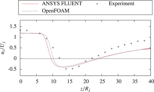
Figure 8. Comparison of the velocity distributions in the main flow direction of the continuous phase in the CBB from simulations in ANSYS FLUENT and OpenFOAM and experiments according to Borée et al. (2001).

Note: The baseline locations of the profiles are at .

In Figure 7 the development of the velocity along the symmetry line is illustrated. The stagnation points are located at the intersections of the curves with . The plot shows that the CFD simulations predict stagnation points which are somewhat shifted compared to the experiment. S₁ lies in front of the experimentally determined one, mainly due to the sharp decline of the normalized velocity. The increase of speed in the second part is clearly lower in the simulations. On the other hand, the stagnation point S₂ in the simulations is shifted downstream with respect to the experimental observations. Correspondingly the increase in speed for in both simulations is significantly lower than in the experiment (note that the curves from OpenFOAM and ANSYS FLUENT are nearly identical).

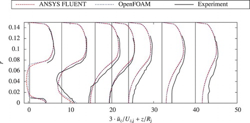
The development in the velocity profiles in the main flow direction as a function of the span-wise coordinate in the experiment and the numerical simulations is shown in Figure 8. Here the circumferential average of the normalized mean axial velocity is given. In agreement with the results in Figure 7, in both numerical simulations the axial velocity at the center line () lags behind the experimental values, especially downstream from the stagnation point S₂ (). Accordingly, the span-wise velocity profiles from the experiment and the numerical simulations show some differences, whereas there are almost no discrepancies between the profiles from OpenFOAM and ANSYS FLUENT.

The near-axis flow region of the central jet accelerates faster in the experiment than in the simulations, therefore momentum transfer through the shear layers from the outer region to the central flow region must be larger. This effect should correlate with a stronger suction from the annular jet into the central jet flow; however, this cannot be seen due to the incomplete velocity profiles in the experiment, which do not resolve the annular jet completely. We assume that the under-prediction of the momentum transfer is mainly due to the RANS turbulence modeling, because similar differences between the experimental and RANS-modeled wake flows have been reported elsewhere (e.g., Iaccarino, Ooi, Durbin, & Behnia, 2003).

5.3.2. Dispersed phase

Figure 9 gives a comparison of the particle velocity profiles after of flow time. At that moment, particles have already spread far into the downstream flow domain. The particle velocity is again analyzed in bands around the corresponding profile baseline, as described in section 4.3.2 above. Here the evaluation band width is set to .

Figure 9. Comparison of the velocity distributions in main flow direction of the dispersed phase in the CBB from simulations in ANSYS FLUENT and OpenFOAM and experiments according to Borée et al. (2001).

Note: Baseline locations of the profiles are at .

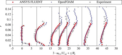
For the central jet flow and the inner shear layers region, good overall agreement between the profiles from the experiment and both numerical simulations is found. Note that the differences between the experimental and numerical particle velocity profiles for the region downstream of stagnation point S₂ are significantly lower than for the fluid flow velocity profiles in Figure 8.

On the contrary, noticeable differences are found in the annular jet and outer shear layer profiles. From the experiments it must be expected that particle dispersion from the inner shear layer through the outer shear layer into the annular jet region should occur. This behavior is qualitatively resolved, but clearly overestimated in the OpenFOAM simulation. The profile at shows that particles are already dispersed into the annular jet. However, in the simulation with ANSYS FLUENT such dispersion is again weaker than in the experiments. In all the profiles, no particles are found in the region , thus the results of the CBB test case confirm the findings from the BFS test case for the dispersion modeling in the case of two-way coupling.

6. Summary and conclusion

In the present study, the capabilities for modeling dispersed particle-laden gas flows with the CFD software packages OpenFOAM 2.1.x and ANSYS FLUENT 14.5 were benchmarked. The numerical models examined are based on the RANS equations for the continuous fluid phase in combination with the stochastic discrete random walk model for the dispersed phase. In the simulations, the coupling between the phases is either one- or two-way; four-way coupling with particle–particle contacts is not treated. Physical models and numerical methods were selected to be as similar as possible in both CFD programs.

The performance of the numerical models is evaluated with the help of two well-known test cases for dispersed particle-laden flows: the backward facing step (BFS) and the confined bluff body (CBB). Both test cases are well documented and have been investigated frequently in the past. The BFS flow is simulated on two- and three-dimensional meshes with one- and two-way coupling between the fluid and the dispersed phase, the CBB flow is simulated with two-way coupling only.

In both test cases, the numerically modeled fluid flow fields are in very good agreement. The continuous phase is adequately captured by the model, as evidenced by the comparison with the experimental data. Differences between the calculated flow data and corresponding information from the experimental measurements are within the well-known uncertainty of the Reynolds-averaged approach of fluid flow model equations.

In the BFS case, the results of the particulate phase from both CFD programs correspond well with the experimental data. The particle velocities and particle positions fit with the experimental data in both the core flow and the shear layer region. Differences between the calculated and measured particle positions and velocities are found in the shear layer between the core flow and the recirculating region past the step. ANSYS FLUENT under-predicts the particle transport in the span-wise direction behind the step due to turbulent dispersion. On the contrary OpenFOAM overestimates the dispersion and predicts lower velocities compared to the experiment. For both programs the applied coupling scheme only had a minor impact on the results. Due to the low volume and mass loading, the momentum transfer is primarily from the continuous phase to the dispersed phase.

From the ANSYS FLUENT results it is apparent that the computational domain has to be three-dimensional when turbulent particle-laden flow is simulated, even if it is reasonable to assume a two-dimensional fluid flow structure. For the two-dimensional case the spreading of the particle cloud is strongly underrated because the three-dimensional character of turbulent dispersion is neglected.

In case of two-way coupling for the CBB, similar observations are made. In the core flow region, the particle velocities and particle positions predicted with both OpenFOAM and ANSYS FLUENT fit well with the experimental data. However, the experimentally observed particle dispersion from the particle-laden central jet through the shear layer to the particle-free annular jet is again over-predicted by OpenFOAM. In the ANSYS FLUENT simulation, the particles remain in the core region around the central jet.

The results of this study imply that both ANSYS FLUENT and OpenFOAM are able to simulate turbulent dispersed particle-laden gas flow for one- and two-way coupling. For the investigated volume loadings it is acceptable to use a one-way coupling. To reliably predict the particle dispersion, the problem should be simulated in three dimensions. The three-dimensional character of turbulent dispersion is neglected if only two dimensions are considered in the simulated problem, which results in an unrealistic particle motion. However, for every engineering problem it is recommended that the CFD model be validated in order to determine performance.

Acknowledgements

Thanks go to Kilian Fröhlich for his beneficial assistance.

Disclosure statement

No potential conflict of interest was reported by the authors.

ORCID

Franziska Greifzu http://orcid.org/0000-0003-3332-1161

References

- Alletto, M., & Breuer, M. (2012). One-way, two-way and four-way coupled LES predictions of a particle-laden turbulent flow at high mass loading downstream of a confined bluff body. International Journal of Multiphase Flow, 45, 70–90. doi: 10.1016/j.ijmultiphaseflow.2012.05.005
- ANSYS FLUENT, 14.5. (2014). User's and theory guide. Canonsburg, Pennsylvania, USA: ANSYS, Inc.
- Anwar-ul-Haque, F. A., Yamada, S., & Chaudhry, S. R. (2007). Assessment of turbulence models for turbulent flow over backward facing step. Proceedings of the World Congress on Engineering (Vol. 2, pp. 2–7). London, United Kingdom.
- Apte, S., Mahesh, K., Moin, P., & Oefelein, J. (2003). Large-eddy simulation of swirling particle-laden flows in a coaxial-jet combustor. International Journal of Multiphase Flow, 29(8), 1311–1331. doi: 10.1016/S0301-9322(03)00104-6
- Armaly, B. F., Durst, F., Pereira, J. C., & Schönung, B. (1983). Experimental and theoretical investigation of backward-facing step flow. Journal of Fluid Mechanics, 127, 473–496. doi: 10.1017/S0022112083002839
- Balachandar, S. (2009). A scaling analysis for point–particle approaches to turbulent multiphase flows. International Journal of Multiphase Flow, 35(9), 801–810. doi: 10.1016/j.ijmultiphaseflow.2009.02.013
- Balachandar, S., & Eaton, J. (2010). Turbulent dispersed multiphase flow. Annual Review of Fluid Mechanics, 42, 111–133. doi: 10.1146/annurev.fluid.010908.165243
- Borée, J., Ishima, T., & Flour, I. (2001). The effect of mass loading and interparticle collisions on the development of the polydispersed two-phase flow downstream of a confined bluff body. Journal of Fluid Mechanics, 443, 129–165. doi: 10.1017/S0022112001005134
- Breuer, M., & Alletto, M. (2012). Efficient simulation of particle-laden turbulent flows with high mass loadings using LES. International Journal of Heat and Fluid Flow, 35, 2–12. doi: 10.1016/j.ijheatfluidflow.2012.01.001
- Burlutskiy, E., & Turangan, C. (2015). A computational fluid dynamics study on oil-in-water dispersion in vertical pipe flows. Chemical Engineering Research and Design, 93, 48–54. doi: 10.1016/j.cherd.2014.05.020
- Chrigui, M., Hidouri, A., Sadiki, A., & Janicka, J. (2013). Unsteady Euler/Lagrange simulation of a confined bluff-body gas–solid turbulent flow. Fluid Dynamics Research, 45(5), 1–27. doi: 10.1088/0169-5983/45/5/055501
- Clift, R., Grace, J., & Weber, M. (2005). Bubbles, drops, and particles. New York, USA: Courier Corporation.
- Corsini, A., Rispoli, F., Sheard, A., Takizawa, K., Tezduyar, T., & Venturini, P. (2014). A variational multiscale method for particle-cloud tracking in turbomachinery flows. Computational Mechanics, 54, 1191–1202. doi: 10.1007/s00466-014-1050-0
- Crowe, C. T., Sommerfeld, M., & Tsuji, Y. (1998). Multiphase flows with droplets and particles (2nd ed.). Boca Raton, Florida, USA: CRC Press.
- Deen, N., Van Sint Annaland, M., Van der Hoef, M., & Kuipers, J. (2007). Review of discrete particle modeling of fluidized beds. Chemical Engineering Science, 62, 28–44. doi: 10.1016/j.ces.2006.08.014
- Elghobashi, S. (1994). On predicting particle-laden turbulent flows. Applied Scientific Research, 52(4), 309–329. doi: 10.1007/BF00936835
- Fessler, J. R., & Eaton, J. (1999). Turbulence modification by particles in a backward-facing step flow. Journal of Fluid Mechanics, 394, 97–117. doi: 10.1017/S0022112099005741
- Hardalupas, Y., Taylor, A. M., & Whitelaw, J. H. (1992). Particle dispersion in a vertical round sudden expansion flow. Proceedings of Royal Society, (pp. 411–442). London: United Kingdom.
- Hishida, K., & Maeda, M. (1991). Turbulence characteristics of particle-laden flow behind a reward facing step. ASME FED, (pp. 207–212). Portland: Oregon.
- Iaccarino, A., Ooi, A., Durbin, P., & Behnia, M. (2003). Reynolds averaged simulations of unsteady separated flow. International Journal of Heat and Fluid Flow, 24, 147–156. doi: 10.1016/S0142-727X(02)00210-2
- Kim, B., Ng, D., Mentzer, R., & Mannan, M. (2012). Modeling of water-spray application in the forced dispersion of LNG vapor cloud using a combined Eulerian-Lagrangian approach. Industrial & Engineering Chemistry Research, 51, 13803–13814. doi: 10.1021/ie3003864
- Kulick, J. D., Fessler, J. R., & Eaton, J. K. (1994). Particle response and turbulence modification in fully developed channel flow. Journal of Fluid Mechanics, 277, 109–134. doi: 10.1017/S0022112094002703
- Laín, S., & Sommerfeld, M. (2012). Numerical calculation of pneumatic conveying in horizontal channels and pipes: Detailed analysis of conveying behaviour. International Journal of Multiphase Flow, 39, 105–120. doi: 10.1016/j.ijmultiphaseflow.2011.09.006
- Launder, B., & Spalding, D. (1974). The numerical computation of turbulent flows. Computer Methods in Applied Mechanics and Engineering, 3(2), 269–289. doi: 10.1016/0045-7825(74)90029-2
- Lin, N., Lan, H., Xu, Y., Dong, S., & Barber, G. (2015). Effect of the gas-solid two-phase flow velocity on elbow erosion. Journal of Natural Gas Science and Engineering, 26, 581–586. doi: 10.1016/j.jngse.2015.06.054
- Maeda, M., Kiyota, H., & Hishida, K. (1982). Heat transfer to gas-solids two-phase flow in separated, reattached, and redevelopment regions. Proceedings of 7th International Heat Transfer Conference, (pp. 249–254). Munich, Germany.
- Mallouppas, G., & van Wachem, B. (2013). Large eddy simulations of turbulent particle-laden channel flow. International Journal of Multiphase Flow, 54, 65–75. doi: 10.1016/j.ijmultiphaseflow.2013.02.007
- Menter, F. (1994). Two-equation eddy-viscosity turbulence models for engineering applications. AIAA Journal, 32(8), 1598–1605. doi: 10.2514/3.12149
- Minier, J.-P., Peirano, E., & Chibbaro, S. (2004). PDF model based on Langevin equation for polydispersed two-phase flows applied to a bluff-body gas-solid flow. Physics of Fluids, 16(7), 2419–2431. doi: 10.1063/1.1718972
- Mohanarangam, K., & Tu, J. Y. (2007). Two-fluid model for particle-turbulence interaction in a backward-facing step. AIChE Journal, 53(9), 2254–2264. doi: 10.1002/aic.11248
- Morsi, S., & Alexander, A. (1972). An investigation of particle trajectories in two two-phase flow systems. Journal of Fluid, 55(2), 193–208. doi: 10.1017/S0022112072001806
- Oefelein, J. C., Sankaran, V., & Drozda, T. G. (2007). Large eddy simulation of swirling particle-laden flow in a model axisymmetric combustor. Proceedings of the Combustion Institute, 31, 2291–2299. doi: 10.1016/j.proci.2006.08.017
- OpenFOAM. (2014). User Guide (2nd ed.). OpenCFD Ltd.
- Patankar, S. V., & Spalding, D. B. (1972). A calculation procedure for heat, mass and momentum transfer in three-dimensional parabolic flows. International Journal of Heat and Mass Transfer, 15, 1787–1806. doi: 10.1016/0017-9310(72)90054-3
- Portela, L., & Oliemans, R. (2006). Possibilities and limitations of computer simulations of industrial turbulent dispersed multiphase flows. Flow Turbulence Combustion, 77, 381–403. doi: 10.1007/s10494-006-9051-5
- Sardina, G., Schlatter, P., Brandt, L. P., & Casciola, C. (2012). Wall accumulation and spatial localization in particle-laden wall flows. Journal of Fluid Mechanics, 699, 50–78. doi: 10.1017/jfm.2012.65
- Saffari, H., & Hosseinnia, S. (2009). Two-phase Euler-Lagrange CFD simulation of evaporative cooling in a wind tower. Energy and Buildings, 41, 991–1000. doi: 10.1016/j.enbuild.2009.05.006
- Sommerfeld, M. (1995). Modellierung und numerische Berechnung von partikelbeladenen Strömungen. Habilitationsschrift. Universität Erlangen: Shaker-Verlag.
- Sommerfeld, M., & Qiu, H.-H. (1993). Characterization of particle-laden, confined swirling flows by phase-doppler anemometry and numerical calculation. International Journal of Multiphase Flow, 19(6), 1093–1127. doi: 10.1016/0301-9322(93)90080-E
- Sommerfeld, M., von Wachem, B., & Oliemans, R. (2008). Best practice guidelines for computational fluid dynamics of dispersed multiphase flows. European Research Community On Flow, Turbulence and Combustion.
- Subramaniam, S. (2013). Lagrangian-Eulerian methods for multiphase flows. Progress in Energy and Combustion Science, 39, 215–245. doi: 10.1016/j.pecs.2012.10.003
- Thangam, S., & Speziale, C. G. (1992). Turbulent flow past a backward-facing step: A critical evaluation of two-equation models. AIAA Journal, 30(5), 1314–1320. doi: 10.2514/3.11066
- Torti, E., Sibilla, S., & Raboni, M. (2013). An Eulerian-Lagrangian method for the simulation of the oxygen concentration dissolved by a two-phase turbulent jet system. Computers and Structures, 129, 207–217. doi: 10.1016/j.compstruc.2013.05.007
- van Vliet, E., Singh, M., Schoonenberg, W., van Oord, J., van der Plas, D., & Deen, N. (2013). Development and validation of Lagrangian-Eulerian multi-phase model for simulating the argon stirred steel flow in a ladle with slag. Proceedings of the 5th International Conference on Modelling and Simulation of Metallurgical Processes in Steelmaking, STEELSIM. Ostrava, Czech Republic.
- Vreman, A. (2015). Turbulence attenuation in particle-laden flow in smooth and rough channels. Journal of Fluid Mechanics, 773, 103–136. doi: 10.1017/jfm.2015.208
- Wang, B., Manhart, M., & Zhang, H. (2011). Analysis of inertial particle drift dispersion by direct numerical simulation of two-phase wall-bounded turbulent flows. Engineering Applications of Computational Fluid Mechanics, 5(3), 341–348. doi: 10.1080/19942060.2011.11015376
- Weber, R., Schaffel-Mancini, N., Mancini, M., & Kupka, T. (2013). Fly ash deposition modelling: Requirements for accurate predictions of particle impaction on tubes using RANS-based computational fluid dynamics. Fuel, 108, 586–596. doi: 10.1016/j.fuel.2012.11.006
- Zhou, Z. Y., Kuang, S. B., Chu, K. B., & Yu, A. B. (2010). Discrete particle simulation of particle-fluid flow: model formulations and their applicability. Journal of Fluid Mechanics, 661, 482–510. doi: 10.1017/S002211201000306X
- Zhu, H., Zhou, Z., Yang, R., & Yu, A. (2007). Discrete particle simulation of particulate systems: Theoretical developments. Chemical Engineering Science, 62, 3378–3396. doi: 10.1016/j.ces.2006.12.089