A CFD and experimental study on cavitation in positive displacement pumps: Benefits and drawbacks of the ‘full’ cavitation model

ABSTRACT

To fill the gap in the literature in terms of numerical studies of positive displacement (PD) pumps in a cavitating condition, a comprehensive and transient computational fluid dynamics (CFD) model of a PD pump, simulating the cavitation arising during the suction stroke, was created. The ‘full’ cavitation model was utilized to study its capability on PD pump cavitation. A set of three plunger speeds were simulated. Using the highest plunger speed, an assessment was made of the effect of 1.5, 3, 4.5 and 15 parts per million (ppm) of air mass fraction on pump performance and cavitation. An experimental test rig, replicating the CFD model, was designed and built in order to validate the numerical model and find its weaknesses. CFD modeled, in a consistent way, the fluid dynamics phenomena related to cavitation (the chamber pressure approaching the vapor pressure, the vaporization/condensation and the pressure spike occurrence at the end of the suction stroke marking the end of cavitation). On the other hand the CFD pressure trends calculated appeared stretched along the time axis with respect to the experimental data, and this highlighted issues in the multiphase and cavitation models: the vaporization/condensation rate calculated by CFD did not follow the real dynamics correctly because the non-condensable gas expansion was overestimated. This was seen when comparing the CFD/experimental results where the simulated pressure drop gradient at the beginning of the suction stroke and the pressure peaks as the valve closed exhibited a delay in their occurrence. The simulation results were sensitive to the dissolved air mass fraction as the delay depended on the amount of air dissolved in the water. Although the influence of the air mass fraction was considered consistent, the 3 ppm CFD case was the closest to the experimental results, whereas the analyst expected the 15 ppm case to be more accurate.

KEYWORDS:

• cavitation in PD pumps
• air fraction and cavitation
• experimental validation of cavitation CFD model
• full cavitation model

Introduction

Positive displacement (PD) pumps have been overlooked by most users for years, even though they may offer significant opportunities to improve processes, enhance efficiency and reduce costs (Parker, 1994). Nowadays PD pumps are becoming essential in some technologies, such as hydraulic fracturing, where centrifugal pumps cannot be used. The performance in terms of achievable maximum pressure and a mass flow rate independent from the pressure head makes PD pumps the most suitable device for this kind of activity (Tackett, Cripe, & Dyson, 2008). On the other hand the design of PD pumps has not changed significantly over the years and the needs of the end user in terms of performance increment (e.g., mass flow rate) are becoming increasingly important. This has led the manufacturers to revise the design of PD pumps to make them compatible with the requirement for better performance in the head and flow rate and a longer operating life, qualities which characterize a competitive device on the market.

Increasing the mass flow rate often means accelerating the plunger by means of increasing the crankshaft angular speed. In many cases this leads to problems related to the decrement of the net positive suction head available (NPSHa) and the increment of the velocity flow through the inlet valve, which may become unacceptably high and cause cavitation damage (Eisenberg, 1963), as well as causing also erosion in the cases where slurry is being pumped. The damage caused by these two phenomena is usually restricted to the inlet valve, which may quickly lose its sealing property in a manner similar to that which Price, Smith, and Tison (1995) observed. This will affect the volumetric efficiency of the device, forcing the end user to stop the process in order to replace the worn valves and valve seats. Decreasing cavitation and erosion under operating conditions leads to a longer life valve, resulting in reduced costs for the end user. Many authors (Johnston, 1991; Shu, Burrows, & Edge, 1997) in the past have studied PD pumps by means of analytic methods such as 1D lumped parameter models. Johnston's model, for instance, was composed “of a number of inter-linked mathematical models representing the pump components”. Although simplified, Johnston's model accounted for the complete transient fluid dynamics of pumping, it was also equipped with a sub-model accounting for the cavitation effects. Very few of them (Ragoth & Nataraj, 2012) have used CFD instead. Ragoth for example carried out a study on the performance of PD pumps by means of CFD but his model was simplified too much as the effect of the valve was not simulated but modelled using a User Defined Function. Ragoth also neglected the compressibility of the working fluid as his model was not multiphase. It is clear that a gap in the literature exists, the authors of this paper aim to fill this gap with the current paper. To date, in fact, no comprehensive CFD models, such as the one described in this paper, have been reported in the technical literature.

This paper discusses the validity of a numerical tool based on CFD which analysts may use to support designers in creating longer-lasting valves and valve seats by reducing cavitation during the suction stroke of positive displacement pumps. The model simulates the transient behavior of a PD pump working in cavitating conditions throughout the inlet stroke. It is realistic because it represents the real fluid dynamics of the pump. The main achievements can be summarized as follows:

1. Self-actuated valves. The inlet valve is not actuated by the user but it moves when the pressure field, calculated by the solver, generates a force sufficient to exceed the valve-spring preload.

2. Moving mesh. The plunger displacement is simulated by means of cell layer creation. During the simulation, the volume of the pump chamber increases. The valve also moves so that the space between the valve and the valve seat increases when the valve lifts off the seat and diminishes when the valve returns to the seat.

3. Multiphase and cavitation model. The mixture multiphase model was utilized to handle the interaction between the water and the vapor. The interphase change rate was calculated by the ‘full’ cavitation model, discussed in the next paragraph.

4. Effect of the non-condensable gas. The cavitation model accounts for the presence of non-condensable gas which interacts with the cavitation.

The capabilities of the CFD model were tested by means of experimental validation. The test rig employed, described below, was fully consistent with the CFD model and represented the same pumping system under the same operating conditions.

Experimental test rig

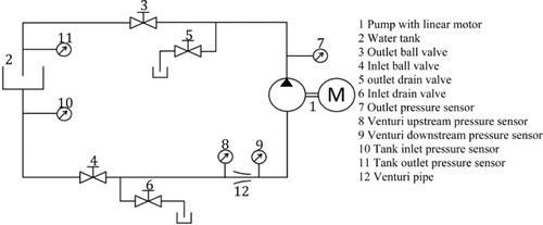
Figure 1 shows the layout of the test rig pumping system. Water, at ambient conditions, flowed from the water tank to the PD pump through a Venturi pipe equipped with two pressure sensors. These transducers provided the pump inlet pressure signal and also the mass flow rate, as the pressure drop across the Venturi pipe is proportional to the mass flow rate due to Bernoulli's effect. After flowing into the pump chamber, the water was pumped back to the water tank via the outlet pipe in a closed loop system. A pressure sensor acquired the outlet pressure close to the pump outlet flange. The water tank had an opening to the exterior to provide it with ambient pressure during the tests. Two pressure sensors placed in the vicinity of the inlet and outlet pipe connections ensured that the oscillation of the pressure at the inlet and outlet was negligible during the test. The inlet and outlet pipes were fitted with two ball valves which had the purpose of isolating the water tank from the pump when it was necessary to drain the pump without draining the whole system. During the tests, Ball Valves 3 and 4 were always wide open whereas Ball Valves 5 and 6 (the drain ball valves) were always closed.

Figure 1. Test-rig schematic.

Note: The pumping system is shown but the pressure sensors on the pump are not shown.

A high-performance linear servomotor was chosen to drive the pump plunger, which was aligned with and coupled to the motor shaft. The motor was controlled by the software provided with the motor, and a closed loop fully automatic system ensured that the displacement produced by the linear motor was the same as the one commanded by the driver software.

Apart from the pressure sensor specified in Figure 1, two additional sensors were placed on the pump. These transducers acquired the pressure within the pump chamber and in the valve-seat lift volume (Figure 2). These locations were identified as the most significant for defining the fluid dynamics phenomena occurring in the pump. In fact:

• The chamber pressure trend denotes the effectiveness of the decompression carried out by the plunger displacement. The slope of the pressure drop during the induction stroke provides evidence of how the air mass fraction dissolved in the water is slowing down the formation of vapor (Iannetti, Stickland, & Dempster, 2014a).

• The valve-seat pressure trend describes the interaction between the chamber and the inlet manifold pressure as it drives the dynamic pressure due to the high velocity which characterizes the flow in between the valve and the seat. The valve-seat lift volume is the zone where flow cavitation is initiated (Opitz & Schlücker, 2010).

Figure 2. Section of the PD pump on the symmetry plane.

Note: The chamber and valve-seat pressure sensor locations are shown (top and bottom detailed view, respectively) and the inspection window on the right of the bottom (suction) valve is shown.

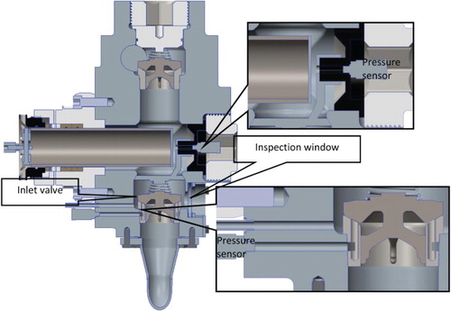
Figure 2 shows the section of the pump taken on the symmetry plane. The top detailed view shows the location of the chamber pressure sensor, which was screwed into a threaded hole cut in the side closing cup of the pump's external case. The tapping location was very close to the top dead center (TDC) position of the plunger. The bottom detailed view shows that four holes were drilled in the valve seat (two visible in the section). An annular recess and a hole in the pump's external case created a path between the valve-seat volume and the pressure sensor, which is shown on the far left side of the bottom detailed view. A transparent inspection window is visible to the right of the bottom (suction) valve. A high-speed camera was placed in front of the inspection window to take pictures of the lifting valve and vapor bubbles.

Table 1 shows the characteristics of the pressure sensors used during the tests. The signals from the transducers were acquired by a National Instruments CompactRio data acquisition system and processed via a real-time National Instruments Labview program. The acquisition frequency for all the signals was 1 kHz. Tap water was utilized to fill the tank and 15 parts per million (ppm) of air mass fraction content in the water can be assumed, as the tank was at ambient conditions. However, the air content was not measured.

Table 1. Pressure sensor characteristics summary.

Pressure sensor	Range (bar)	Absolute/ Relative	Maximum non-linearity [%]	Response time [ms]
Venturi Upstream	0–2.5	A
Venturi downstream	0–2.5	A
Chamber pressure	0–10	R
Valve-seat pressure	0–10	A	0.25	<0.5
Pressure outlet	0–6	A
Tank inlet	0–0.25	R
Tank outlet	0–0.25	R

Each test was carried out twice in order for the high-speed camera to record the motion of the inlet valve with a frame rate of 1000 and 500 frames per second (fps). According to the specifications of the camera utilized, in fact, the 500 fps sequence allowed a wider view of the valve whereas the 1000 fps sequence gave a much more detailed view of the phenomena occurring in the valve-seat gap. The 500 fps sequence was utilized to visualize the valve together with the flow downstream from the valve while the 1000 fps sequence was utilized to see only the flow through the valve. The 1 kHz frames were also used to measure the valve lift by an in-house post-processing program which measured the valve lift by comparing the displacement of a reference mark from the initial frame (zero lift) to the mark's location on subsequent frames.

It has to be noted that the analyst did not manage to accurately measure the mass flow rate because the Venturi pipe pressure sensors were very sensitive to the pressure waves and electromagnetic interference. The authors leave the improvement of the mass flow acquisition for the future research discussed in this paper.

Experimental tests

Different from real applications, where the plunger is usually driven by a rotational motor/engine and the displacement of the plunger is operated by a crankshaft (Miller, 1995), in this work the plunger motion was operated by means of a linear motor controlled by its software (Figure 3). Three tests at three different plunger speeds were carried out. In each test of Figure 3 the displacement-time history was fixed by a piecewise polynomial function composed of:

1. A constant acceleration part of 4, 5.5 and 7 m/s² for Tests 1, 2 and 3, respectively.

2. A constant velocity part of 0.8, 0.95 and 1.1 m/s for Tests 1, 2 and 3, respectively.

3. A constant deceleration part of 4, 5.5 and 7 m/s² for Tests 1, 2 and 3, respectively.

Figure 3. Plunger displacements and velocities fed into the motor drive administration software are shown.

The plunger stroke in all of the tests was 0.204 m. Figure 3 represents the suction stroke only; the delivery stroke, which is not discussed in this paper, was carried out slowly and only to reposition the plunger to the TDC position again, ready for the next test. The acceleration and velocity were designed to achieve the incipient, partial and full cavitation regimes (Iannetti, Stickland, & Dempster, 2015; Opitz & Schlücker, 2010; Opitz, Schlücker, & Schade, 2011).

CFD model

Geometry and mesh

The CFD model exactly replicated the design of the test rig, from the water tank to the pump chamber. The outlet valve and pipeline were not modeled, as the CFD model simulated the suction stroke only. The fluid volume was extracted from the solid part which was then decomposed, as per the pattern shown in Figure 4, in order to allow the creation of a hybrid mesh and also to set the moving mesh in the zones affected by the volume change (growing displacement volume due to the plunger motion) and motion (valve lift). The displacement volume growth was simulated by means of hexahedral cell layer creation in the direction of the plunger top surface motion. The plunger displacement volume and valve lift volume were simulated by means of cell layer creation, while the top and bottom volumes enclosing the valve external surfaces were rigidly translated at the same velocity in order to leave the external shape of the valve unchanged during the motion. The top and bottom disks were squeezed and stretched respectively in order to guarantee the mesh continuity across the valve (Figure 5; see also Iannetti, Stickland, & Dempster, 2014b).

Figure 4. Decomposition pattern of the fluid volumes of the pump chamber (Iannetti et al., 2014a).

Note: The numbered items are listed in Table 3.

Figure 5. View of the mesh utilized for the analysis.

Note: The detailed section of the mesh is taken from the valve vicinity.

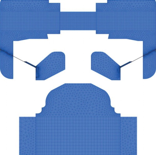
A mesh sensitivity test was carried out to define the proper mesh spacing in order to obtain the most accurate results with the lowest overall number of elements, thereby decreasing the computational cost. Table 2 shows the overall quality and size of the three meshes tested, and Table 3 shows more details of the kind of mesh and size utilized for each fluid volume listed in Figure 4.

Table 2. Mesh sensitivity analysis for three mesh sizes.

Mesh	Number of cells (M)	Average skewness (-)	Approx. computational time (h)
1	3	0.24	48
2	5	0.26	60
3	6	0.22	72

Table 3. Mesh 2 details summary.

Location (see figure 4)	Volume description	Mesh type	Size details min–max [mm]	Mesh motion
1	Valve-seat lift	Hexahedral	0.2–1	Expanding
2	Inlet valve	Wedge	1–3	Compressing
3	Inlet valve	Hexahedral	2–3	Expanding
4	Displacement	Hexahedral	2.5–2.5	Expanding
5	Pump chamber	Tetrahedral	2.5–5	Static
6	Valve internal	Tetrahedral	1–2.5	Translating
7	Inlet manifold	Tetrahedral	2–4	Static
8	Valve top volume	tetrahedral	1–2	Translating

Boundary conditions and valve motion user-defined function (UDF)

A fixed gauge pressure of 0 Pa was utilized as the inlet boundary condition. The fixed displacement motions described by Figure 3 (Tests 1, 2 and 3) were fed into the CFD solver by means of a user-defined function (UDF) which was attached to the plunger top surface moving mesh model to drive the displacement volume change. The valve lift moving mesh was handled by a second UDF attached to the CFD solver. This second program coupled the pressure forces acting on the valve, calculated at the end of each time step, with the valve lift. The algorithm also accounted for the valve-spring force, as the spring stiffness characteristic was introduced into the overall force balance. By means of a first-order Eulerian method, the UDF numerically integrated the overall force acting on the valve (Figure 6). From this force the valve acceleration velocity and displacement were calculated. The displacement was utilized by the valve lift moving mesh algorithm in order to prepare the new mesh for the next time-step operations.

Figure 6. UDF scheme operations (Iannetti et al., 2014b).

CFD sub-models and solver settings

The k-ε turbulence model was used as it provided better convergence over the k-ω model. The enhanced wall treatment was used to correct the standard wall function in cases where the y+ values lay beyond the optimum range for the k-ε model (ANSYS, 2011b).

The mixture model (ANSYS, 2011a) was used for the multiphase model. It was preferred over the other models present in the commercial software used (ANSYS Fluent) because of the low computational cost required. To account for the interphase change due to cavitation, the ‘full’ cavitation model (Singhal, Athavale, Huiying, & Yu, 2002) was switched on. This cavitation model accounts for the effect of the non-condensable gas fraction dissolved in the water in an explicit way within the second phase. The model makes use of the ideal gas law, the pressure calculated by the CFD solver and the air mass fraction input by the user in order to calculate the air volume fraction. Tests 1 and 2 ran with 3 ppm of air mass fraction while the full cavitation test (Test 3) also ran with 1.5, 4.5 and 15 ppm in order to investigate the influence of the mass fraction on cavitation. Dissolved air, in fact, comes out of the solution due to the pressure drop and interferes with cavitation (Wood, Hart, & Ernesto, 1998). Table 4 summarizes the chosen settings.

Table 4. Solver settings summary.

The commercial finite volume software ANSYS Fluent 15 was used as a Reynolds-averaged Navier–Stokes (RANS) solver on an Intel® XEON® CPU E5-1650 v3 @ 3.5 GHz processor with 16 GB RAM. Three days were needed for a single run to simulate the entire suction stroke.

CFD monitors

During the CFD simulation the models were set to monitor every time step and store the data of the following quantities:

1. Chamber pressure: a monitor point close to the TDC position of the plunger was created.

2. Valve-seat pressure: this monitor returned the volume-weighted average of the static pressure in the valve-seat lift volume after every time step.

3. Inlet pressure: this is the static pressure downstream from the Venturi pipe.

4. Mass flow rate.

5. Inlet valve lift.

The monitor locations in the CFD model were set to the same location as the pressure sensors in the experimental rig to allow comparison with the experimental data. It was also decided that the following monitors, which had no counterpart in the experimental test, were of interest for the analysis:

• Valve-seat vapor volume fraction. This is the valve-seat lift volume-weighted average of the vapor fraction.

• Valve-seat air volume fraction. This is the valve-seat lift volume-weighted average of the air fraction which gets out of the solution because of the low static pressure.

Comparison of the CFD model and experimental results

Test 1: incipient cavitation

Test 1 was designed to achieve the incipient cavitation regime by means of low plunger velocity and acceleration, The CFD model was set to 3 ppm of air mass fraction. Figure 7 shows the trend of the chamber and valve-seat static pressure. Figure 7(a) shows that the minimum pressure in the chamber stays sufficiently above the vapor pressure, while Figure 7(b) shows that the valve-seat minimum pressure is always higher than the chamber pressure. This is evidence of incipient cavitation. In fact, a small amount of vapor generation cannot be excluded, as the static pressure could approach the vapor pressure locally in zones of high velocity or turbulence. Figure 8(a) shows how the CFD model estimates the composition of the second phase volume fraction in the valve-lift volume. The maximum vapor fraction calculated was 14% and occurred roughly in the middle of the suction stroke. The average results are very low, as the vapor quickly returned to negligible values. This is confirmed by the frame sequence of Figure 9 where a small amount of vapor is detected as, in some frames, the valve is partially obscured by the vapor cloud generated in the vicinity of the exit edge of the valve main body. The slopes of the pressure decrements calculated by the CFD model in both parts of Figure 7 are lower than their experimental counterparts, although the trends are in good agreement in the first half of the suction stroke.

Figure 7. (a) Pump chamber static pressure and (b) valve-seat static pressure for the experimental and CFD model results of Test 1.

Note: The CFD model was run with 3 ppm air content in the water.

Figure 8. (a) Second phase fraction composition according to the CFD model and (b) valve lift for the experimental and CFD model results of Test 1.

Note: The CFD model was run with 3 ppm air content in the water.

Figure 9. Null/incipient cavitation.

Note: Only three frames show vapor which does not obscure the view of the valve.

Pressure spikes affect the second half of the suction stroke. They are present in both the experiment and the CFD plots, although the latter show a delay in the spike's occurrence. It would appear that the CFD pressure trends are stretched along the time axis when compared to the experimental results.

As the CFD is affected by low pressure longer than the experiment, the maximum valve lift achieved by CFD is higher than the experiment (Figure 8(b)), which also shows the delay of the maximum valve lift occurrence compatible with the delay in the occurrence of the pressure spikes shown in Figure 7. Figure 8(b) demonstrates that the pressure spikes are the result of the water hammer effect related to the valve closing, as the spike's temporal location corresponds to the negative valve velocity location in the valve-lift trend in both the CFD model and the experiment. Errors in estimating the valve dynamics affect the estimation of the pressure peak temporal location. However, besides the delay, in this case the trends are in good agreement with each other.

Test 2: partial cavitation

Test 2 was designed to achieve the partial cavitating conditions. The CFD model was set to 3 ppm of air mass fraction (as with Test 1). Figure 10 shows that the static pressure in both the chamber and the valve-seat locations were closer to the vapor pressure for a longer time, in the first half of the suction stroke, than in Test 1. The CFD model lines are again shifted with respect to the experimental results but the trends are in good agreement with each other from a qualitative view. In this test, the CFD model predicts the water hammer effect but the magnitude of the resulting pressure spikes is larger than in Test 1.

Figure 10. (a) Pump chamber static pressure (log scale) and (b) valve-seat static pressure (log scale) for the experimental and CFD model results of Test 2.

Note: The CFD model was run with 3 ppm air content in the water.

Also in this case, because the CFD model's low pressure lasts longer than that of the experiment, it may be assumed that the pressure forces across the valve created the lift force for a longer period of time. This resulted in a bigger and delayed valve lift achieved by the CFD model (Figure 11(b)). Figure 11(b) also reveals that the magnitude of the pressure spike was overestimated by the CFD model because of the behavior of the valve lift trend. In fact, while returning to the seat, according to CFD model, the valve reversed its motion once (0.27 s). The experimental trend results are much smoother. It is important to show that the pressure peaks occur a little after the valve reverses the motion and, in the opinion of the authors, the valve reverse motion is the actual cause of the pressure spikes.

Figure 11. (a) Second phase fraction composition according to the CFD model and (b) valve lift for the experimental and CFD model results of Test 2.

Note: The CFD model was run with 3 ppm air content in the water.

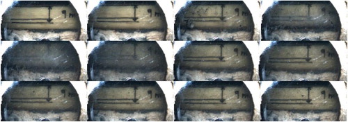
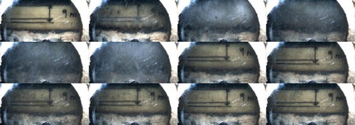
The maximum vapor fraction in the valve-seat lift volume, estimated by the CFD model was 14% for Test 2 (Figure 11(a)). This is similar to the result of Test 1, but the maximum level was kept for more than one third of the overall suction stroke duration. Figure 12 shows twelve frames, evenly separated, taken by the high-speed camera. The vapor generation is demonstrated to be non-negligible as in two of the images the valve is completely obscured by the vapor cloud.

Figure 12. Partial cavitation.

Note: Four frames show a vapor cloud around the valve-lift gap; in two of them, the view of the valve is obscured almost completely.

Test 3: full cavitation

Test 3 involved the highest plunger speed and was designed to achieve the full cavitating condition (for details, see Opitz & Schlücker, 2010). For this test, the CFD simulations were run four times with 1.5, 3, 4.5 and 15 ppm of air mass fraction to shed light on the sensitivity of the CFD model solution to the air content in the water.

Figure 13 shows the trend of the chamber pressure and the valve-seat lift volume static pressure. Both cases highlight a flat and low pressure which affects the first half of the suction stroke. During the first part of the suction stroke, the experimental line and the 1.5 ppm CFD lines overlap in Figure 13(b). The same lines are very close to each other in Figure 13(a). High-magnitude pressure spikes affected the second half of the suction stroke. The water hammer effects, in the experimental case, produced lower magnitude pressure spikes with respect to the CFD model lines. Figure 14 was obtained by the CFD model analysis and shows the vapor volume fraction and the air volume fraction in the valve-seat lift volume. The figure shows that the higher the air content, the lower the vapor generation – and this is in agreement with what was postulated by Iannetti et al. (2014a). In this case, the magnitude of the pressure peaks (Figure 13) was overestimated by the CFD model because of the valve bounces visible in Figure 15. The peak's magnitude is predicted by all of the CFD lines but the occurrence was affected by a delay, as with Tests 1 and 2. Figure 13 shows that the delay was affected by the air mass fraction The higher the air mass fraction, the bigger the delay in the occurrence of the pressure spike for the CFD model. Furthermore, the higher the air mass fraction, the farther away from each other the pressure lines lay (i.e., the 3, 4.5 and 15 ppm CFD model lines of Figure 13). The 1.5 ppm curve produced the closest fit to the experimental line whereas the 15 ppm line shows the biggest delay.

Figure 13. (a) Pump chamber static pressure and (b) valve-seat static pressure for the experimental and CFD model results of Test 3 demonstrating the sensitivity of the CFD model to the air mass fraction.

Figure 14. (a) The vapor volume fraction in the valve-seat lift volume and (b) the air volume fraction in the valve-seat lift volume according to the CFD model of Test 3.

Figure 15. Valve lift for the experimental and CFD model results of Test 3 demonstrating the sensitivity of the CFD model to the air mass fraction.

A similar correlation between the air content and the net positive suction head required (NPSHr) which affects vapor cavitation was also observed in a study conducted on centrifugal pumps (Ding, Visser, & Jiang, 2012).

As the air expansion, shown by Figure 14(b), reveals a second peak after it reaches the zero volume fraction value around 0.25 s, it may be assumed that the valve bounces on and off the seat once before completely closing. This is confirmed by the valve lift trend of Figure 14. The 3 and 4.5 ppm CFD simulations clearly show that the valve touches the seat after 0.3 s and then lifts off it before closing completely at the end of (or a little after) the suction stroke. The 1.5 ppm simulation does not follow exactly the same pattern, as in this case the valve reverses the motion at 0.27 s before touching the seat. The 15 ppm curve does not show the same behavior as, for this case, the valve closes approximately at the same time as the plunger motion comes to the end.

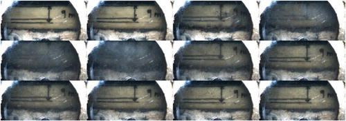
The valve lift experimental trend deserves further discussion. The sequence of images shown in Figure 16 demonstrates the large amount of vapor generated. In four frames out of twelve, in particular, the valve was not visible because of the significant amount of vapor bubbles, which is clear evidence of full cavitation. In these frames the graphical post-processing program, which estimated the valve lift, failed and caused the gap in the experimental valve lift data (Figure 15). However, the maximum valve lift can be estimated by interpolation and assessed as ranging between 3 and 3.5 mm, which demonstrates that the CFD model, once again, overestimated the maximum valve lift. As discussed for Tests 1 and 2, the reason for the overestimation of the valve lift is the longer application of the lifting pressure force on the valve. Furthermore, until 0.1 s, the 1.5 ppm CFD simulation follows the experimental valve lift trend closely, while the 15 ppm case is the least accurate, even though 15 ppm was expected to be the real air content in the water utilized (tap water). The 3 and 4.5 ppm cases lie consistently in between the 1.5 and 15 ppm cases.

Figure 16. Full cavitation.

Note: Five frames show a vapor cloud around the valve-lift gap; in four of them, the view of the valve is completely obscured.

Figure 17 shows the spectrum of the chamber pressure signals of Figure 13(a), from which the following remarks can be observed:

1. Besides the pumping frequency, the experimental line shows two high-power frequencies which are not sufficiently damped. Above 10 Hz, the spectrum presents two more peaks which are barely visible (20 and 33 Hz). This means that, in the specific test case, the wave energy dissipation due to the turbulence is more effective above 15 Hz.

2. The 15 ppm results clearly show the behavior of the system above the critical damping; this means that the multiphase CFD model damped the oscillations much more than in reality, highlighting issues in the physical properties of the mixture (water, air and vapor).

3. The 1.5 ppm results show non-damped high- frequency components. Their presence can be explained by the fact that the turbulence model utilized was not capable of correctly damping the high-frequency components. Comparing these results with the 15 ppm data, it appears that the dampening in the CFD model is provided mainly by the action of the air rather than the main phase (water), which is not capable of providing the physical damping.

4. The 3 and 4.5 ppm CFD model lines follow qualitatively the same trend of the 1.5 ppm line, showing damped components in the spectrum.

Figure 17. FFT of the chamber pressure signals for the experimental and CFD model results of Test 3.

The FFT analysis suggests that the analysis should focus on the modeling and numerical issues associated with the effect of the non-condensable gas on pressure wave prediction.

Highlights of the phenomena observed

Combining the observations of the experimental and numerical data with the discussion of the results in the previous paragraph, the following brief summary can be drawn:

• All the phenomena related to the fluid dynamics of cavitation were predicted by the CFD model (the decompression, the interaction with the non-condensable gas, the vapor generation, and the water hammer pressure peak which marks the end of cavitation). Increasing the plunger velocity resulted in the cavitation regime being worse, as expected. Increasing the air content in the water caused a decrease in the amount of vapor generated. This proves the consistency of the model.

• The CFD model overestimated the valve maximum lift due to overestimating the low-pressure duration. The reason for this is the failure of the cavitation model, which accounts for the influence of the air mass fraction in cavitation. The CFD model overestimated the influence of the expansion of air on cavitation.

• The CFD pressure lines are generally slightly above the experimental lines in the low-pressure region. The CFD also overestimated the magnitude of the pressure spikes (Figures 7, 10 and 13) as a consequence of the incorrect valve velocity trend prediction.

• Although a good match between the experiments and the 15 ppm CFD case was expected, the 1.5 ppm CFD simulations were, in fact, the closest match to the experimental results.

The authors identified the influence of the air expansion on the fluid dynamics of the pump in cavitating conditions. This should be investigated further as, in the opinion of the authors, it is the main cause of the mismatch between the CFD model and the experimental data.

It is clear that the explicit algorithm managing the volume fraction estimation and thus the influence of the air (discussed in the paragraph dedicated to the solver settings) did not perform as required. The numerical model overestimated the expansion of the non-condensable gas during the low-pressure part (the first half of the suction stroke). This affected the amount of time that the recompression (carried out at approximately constant pressure) needed to ‘eliminate’ the air, resulting in a longer application of the lifting force to the valve. Therefore, all the phenomena observed, such as the overestimation of the valve maximum lift and the magnitude and frequency of the pressure peaks, should be considered a direct consequence rather than a further source of problems.

The reason why the air expansion in the mixture is not predicted correctly lies in the assumptions and simplifications made by the cavitation model of Singhal et al. (2002). With regard to the air mass fraction, the only effect accounted for by the model was the volume fraction, which appeared and disappeared according to the pressure value in all the cells of the discrete model. The air volume fraction interacted with the pressure field only indirectly through the second phase volume fraction transport equation. No momentum equation of the air was solved either by the cavitation model or the multiphase mixture model. The energy involved in the air expansion is not present in the fluid dynamic field, as the energy equation was not solved and the mixture momentum equation did not account for the exchange of momentum between the second phase and the primary phase. As a result, the dynamics of the vapor bubbles was not taken into account and the bubbles expanded without any constraint, which explains the results of the 15 ppm CFD simulation. Furthermore, the cavitation model does not account for the dynamics of the bubbles, as the second-order terms of the Rayleigh–Plesset equation are neglected in the cavitation model utilized.

Moreover, there is another aspect the authors would like to point out. During the experiments, no measurement of the dissolved air content was carried out. However, the numerical model assumed the condensation of the entire mass of the dissolved gas. It would be interesting at this point to know whether or not fluid dynamic phenomena (for instance turbulence) can prevent part of the dissolved gas from coming out of the solution and taking part in the expansion of the second phase.

Conclusions and further improvements

An experimental test rig designed to test a PD pump in incipient, partial and full cavitating conditions was designed and built to validate a CFD multiphase model which exactly replicated the test rig and operating conditions. The multiphase model was equipped with the ‘full’ cavitation model, which was tested with air mass fractions of 1.5, 3, 4.5 and 15 ppm. The incipient and partial CFD simulations were run with air content in the water of 3 ppm only. Measurements of chamber static pressure, valve-seat static pressure and valve lift were taken during the experiments and compared with the CFD model results. The analysis revealed good consistency, as the CFD model trends were in good qualitative agreement with the experiments. Given the significant complexity of the problem, the research also resulted in a reasonable level of accuracy which was affected by the unrealistic simulated influence of non-condensable gas expansion. The CFD model demonstrated a smaller gradient of pressure drop at the beginning of the suction stroke, and a certain delay in the pressure spikes occurred in the second part of the suction stroke when the water hammer effect took place as a result of the valve closing. The pressure drop gradient and the delay in the pressure spike occurrence depended on the air mass fraction; the lower the air content, the less the delay and the steeper the pressure gradient. The CFD model always overestimated the valve lift; the CFD model maximum lift was higher and shifted with respect to the experimental lift. The reason for the difference in predicting the lift was the longer application of the lifting pressure force on the valve estimated by the CFD model, which in turn was caused by the slow recompression of the air with respect to the experiment. The main cause of the accuracy loss was found to be the failure of the algorithm within the cavitation model estimating the expansion and compression of the air, and therefore its influence on cavitation. Further investigation on the applicability of the mixture model utilized in this study (ANSYS, 2011a) should be carried out. Also, the air mass fraction, which was handled in an explicit way by the cavitation model, should be treated as a real third phase and solved via a dedicated transport equation in order to strongly couple the phases and account for the momentum exchange between phases. For future improvement, the authors also suggest that the real air content in the water utilized for the experiments should be measured.

An important key parameter which could shed more light on the problem is the volumetric efficiency. This parameter, in fact, is directly related to the cavitation regimes (Iannetti et al., 2015); the lower the volumetric efficiency, the higher the integral of the vapor generated. It is very simply to calculate volumetric efficiency using CFD but very difficult to measure it in an experimental rig. In future, it would be worthwhile completing an experimental analysis and equipping the test rig with an accurate mass flow meter. Once the volumetric efficiency is accurately measured, it can be compared with the CFD model results and assist in isolating the numerical cause which leads to the issues observed and discussed in this paper.

Disclosure statement

No potential conflict of interest was reported by the authors.

References

- ANSYS. (2011a). ANSYS fluent theory guide. ANSYS Inc.
- ANSYS. (2011b). ANSYS fluent UDF manual. ANSYS Inc.
- Ding, H., Visser, F. C., & Jiang, Y. (2012). A practical approach to speed up NPSHR prediction of centrifugal pumps using CFD cavitation model. In Proceedings of the ASME 2012 fluids engineering summer meeting. Puerto Rico, USA: Rio Grande.
- Eisenberg, P. (1963). Cavitation damage. Washington, DC: Office of Naval Research.
- Iannetti, A., Stickland, M. T., & Dempster, W. M. (2014a). An advanced CFD model to study the effect of non-condensable gas on cavitation in positive displacement pumps. In 11th international symposium on compressor & turbine flow systems theory & application areas SYMKOM 2014 IMP2. Lodz, Poland.
- Iannetti, A., Stickland, M. T., & Dempster, W. M. (2014b). A computational fluid dynamics model to evaluate the inlet stroke performance of a positive displacement reciprocating plunger pump. Proceedings of the Institution of Mechanical Engineers, Part A: Journal of Power and Energy, 228(5), 574–584.
- Iannetti, A., Stickland, M. T., & Dempster, W. M. (2015). A CFD study on the mechanisms which cause cavitation in positive displacement reciprocating pumps. Journal of Hydraulic Engineering, 1(1), 47–59.
- Johnston, D. N. (1991). Numerical modelling of reciprocating pumps with self-acting valves. Journal of Systems and Control Engineering, Part I, 87–96. http://doi.org/10.1243/PIME
- Miller, J. E. (1995). The reciprocating pump, theory design and use (2nd ed.). Malabar, FL: Krieger publishing company.
- Opitz, K., & Schlücker, E. (2010). Detection of cavitation phenomena in reciprocating pumps using a high-speed camera. Chemical Engineering & Technology, 33(10), 1610–1614. doi: 10.1002/ceat.201000204
- Opitz, K., Schlücker, E., & Schade, O. (2011). Cavitation in reciprocating positive displacement pumps. In Twenty-seventh international pump users symposium (pp. 27–33). Houston, Texas.
- Parker, D. B. (1994). Positive displacement pumps-performance and application. In 11th International Pump User Symposium.
- Price, S. M., Smith, D. R., & Tison, J. D. (1995). The effects of valve dynamics on reciprocating pump. In Proceedings of the twelfth international pump users symposium (pp. 221–230). Texas A&M University.
- Ragoth, R., Singh, & Nataraj, M. (2012). Study on Performance of Plunger Pump at Various Crank Angle Using CFD. IRACST Engineering Science and Technology: An International Journal (ESTIJ), ISSN:2250-3498, 2(4), 549–553.
- Shu, J., Burrows, C. R., & Edge, K. A. (1997). Pressure pulsations in reciprocating pump piping systems Part 1: modelling. Proc Inst Mech Engrs, 211 Part I(April), 229–237.
- Singhal, A., Athavale, M., Huiying, L., & Yu, J. (2002). Mathematical basis and validation of the full cavitation model. Journal of Fluids Engineering, 124(3), 617–624. doi: 10.1115/1.1486223
- Tackett, H. H., Cripe, J. A., & Dyson, G. (2008). Positive displacement reciprocating pump fundamentals- power and direct acting types. In Proceedings of the twenty-fourth international pump user symposium (pp. 45–58). Texas A&M University.
- Wood, D. W., Hart, R. J., & Ernesto, M. (1998). Application guidelines for pumping liquids that have large dissolved gas content. In Proceedings of the 15th international pump user symposium (pp. 91–98). Huston, TX, USA.