3D shape optimization of fan vanes for multiple operating regimes subject to efficiency and noise-related excellence criteria and constraints

ABSTRACT

Fully generic 3D shapes of centrifugal roof fan vanes are explored based on a custom-developed numerical workflow with the ability to vary the vane 3D shape by manipulating the control points of parametric surfaces and change the number of vanes and rotation speed. An excellence formulation is based on design flow efficiency, multi-regime operational conditions and noise criteria for various cases, including multi-objective optimization. Multiple cases of optimization demonstrate the suitability of customized and individualized fan designs for specific working environments according to the selected excellence criteria. Noise analysis is considered as an additional decision-making tool for cases where multiple solutions of equal efficiency are generated and as an additional criteria for multi-objective optimization. The 3D vane shape enables further gains in efficiency compared to 2D shape optimization, while multi-objective optimization with noise as an additional criterion shows potential to greatly reduce the roof fan noise with only small losses in efficiency. The developed workflow which comprises (i) a 3D parametric shape modeler, (ii) an evolutionary optimizer and (iii) a computational fluid dynamics (CFD) simulator can be viewed as an integral tool for optimizing the designs of roof fans under custom conditions.

KEYWORDS:

• Parametric 3D shape optimization
• centrifugal fan
• CFD
• multi-regime
• multi-criteria

1. Introduction

Roof fans were traditionally considered to be ‘small’ machines and as such did not attract the major interest of the optimization community. Nowadays however, it is obvious that fans are a major energy consumer if one considers their presence on a mass scale (Bertoldi & Atanasiu, 2009).

Beyond this significance, the variable operating conditions of fans and their related distinct excellence criteria and constraints make them a demanding challenge for shape optimization. If the number of vanes is another design variable then this becomes a hybrid discrete–continuous optimum design problem. Moreover, if the operating regimes can be controlled by steering the rotational speed for example, then the respective optimum design problem may become somewhat coupled with the optimum control problem.

The essential principles in optimization and optimum design are well known, including generic optimum design principles, evolutionary procedures and the application of soft computing and their applications (Arora, 1989; Papadrakakis & Lagaros, 2004). These procedures represent one building block of the workflow to be developed in this paper.

Another numerical constituent of the workflow are methods and algorithms from computational geometry and 3D shape modeling entities (Rogers & Adams, 1976). These methods enable dynamic shape modeling to be accommodated into the workflows such that the optimizers can modify the geometry based on the response from computational fluid dynamics (CFD) simulators.

These computational components, numerical optimization procedures, parametric 3D geometry modeling algorithms and CFD simulation methods are here combined in order to numerically embed shape optimization of roof fan vanes. Evolutionary optimization procedures are suitable for such a computational framework as no gradient information is necessary and, being global methods, they are not prone to getting trapped in local optima. Moreover, their inherent slow convergence rates (compared to gradient methods) can be compensated to a certain degree by making use of their natural suitability for computational parallelization. The convergence can be accelerated by using surrogate functions (such as previously trained neural networks). Recent real-life applications of contemporary soft-computing techniques exist in different fields (Chau & Wu, 2010; Taormina & Chau, 2014; Wang, Chau, Xu, & Chen, 2015). Given the fact that the evolutionary optimizers inherently provide for multi-objective optimization by generating full Pareto fronts in a single cycle, they are increasingly becoming the method of choice in many application areas. They also offer convenient techniques for implementing robust and multi-point optimization.

With such potential in mind, the traditional fan design based on a nominal operating point and rotational speed can be replaced with shape optimization using CFD simulation across a range of regimes. This concept makes it possible to optimize for the best total work regime of the fan (as opposed to the peak performance at the nominal point and poor efficiency elsewhere) for a given distribution of the operational regimes.

The procedure developed here involves several essential contributions to optimum fan design. The 3D vane geometry is modeled using B-spline surfaces, which makes it possible for any 3D shape to be modeled by the corresponding adjustment of the relevant parameters. The optimizer is assigned the task to use this design freedom to shape the vanes for maximum energy conversion efficiency.

It was observed through numerical experiments that a number of 3D shapes perform equally or close to equally well in terms of conversion efficiency while being geometrically different. In such cases, another excellence criterion, noise analysis was engaged to arbitrate in terms of ultimate decision-making.

The computational implementation of this complex procedure was facilitated by using components embedded within a numerical workflow. An evolutionary optimizer is in charge of reshaping the vanes, coupled with a CFD simulator in terms of process and data flows. The CFD simulation for all candidate designs is incorporated as a computational service provided by independent software, which is included in the workflow. Optimization for multi-point operating regimes was accomplished by generating a statistical sample of the assumed overall lifespan operational conditions of the fan. The CFD model was validated by extensive laboratory tests by Milas, Vučina, and Marinić-Kragić (2014) to confirm its compliance with the actual performance before being coupled with the optimizer.

Further considerations related to the numerical implementation were necessary up front. The 3D geometry modeling of both global and local variations of the shape is necessary to a certain degree, while using a compact data set of shape parameters. If many shape parameters are used to model the vane geometry, the matching dimensionality of the optimization space may become prohibitively high. On the other hand, too few geometric parameters limit the shape modeling capacity and flexibility, in which case local features in particular may be beyond the modeling potential.

CFD models require the application of appropriate turbulence models and domain discretization since they have a significant impact on the simulation results. The computational workflow must accommodate process flows and the data flows. The former need to be asynchronous for efficiency in parallel environments and the latter involve data mining, which needs to serve the excellence and constraint expressions. For generic fan optimization with prescribed target output pressure and flow rates, additional variables beyond the shape parameters are necessary, as stated above. In particular, the rotational speed of the fan and the number of vanes are also treated as design variables in the overall model.

The paper includes several layers of original development. Completely generic 3D modeling of the vane shape by using parametric surfaces rather than some of the physical parameters of the vanes is the primary contribution of the paper. Parametric surfaces have also been used for modeling the flexible computational domain to extend the range of possible vane shapes. Genetic algorithms have been combined with the Nelder–Mead simplex method in a memetic algorithm to achieve faster convergence to the optimal solution. Lastly the paper deals with the resolution of equally excellent shapes by introducing multi-objective criteria (Deb & Goel, 2002) with elementary noise analysis.

This paper develops a novel approach to shape synthesis by applying generic parametric curves and surfaces as geometric class templates rather than vane-specific physical entities. This approach offers significantly more local and global shape modeling freedom to the optimizer. This geometric model is embedded in the respective optimization workflow along with CFD simulators in the context of multi-regime robust optimization which allows for physically more relevant results than the traditional approach. Furthermore the paper presents elementary noise analysis with multi-objective optimization test cases presenting possible shape modifications to optimize vanes for noise reduction.

The paper is organized according to the following key elements:

• The essentials of the CFD model.

• The parametric modeling of the 3D shape.

• The developed workflow and optimization procedures.

• The different optimization cases, including multi-objective optimization with elementary noise analysis.

• A discussion of the results.

2. Roof fan design and performance

The electricity consumption for fan systems in the residential, tertiary and industrial sector in the European Union (EU) is estimated at 200 TWh/y which is roughly 8% of the total electricity consumption (Radgen, 2002). The efficiency of fans depends on their size and type (centrifugal, axial, mixed flow) but 65 to 70% is an average value for the range of fan powers up to 500 kW. An increase of 10 to 15% in fan efficiency is considered technically feasible (Adnot, Kemna, & Hitchin, 2012). Roof fans are used for the extraction of air from buildings and are generally considered low-power devices. However, their market share is not negligible as they make up 30% of the fan market for non-residential ventilation (industrial and commercial buildings, offices, etc.). Their energy-saving potential is much higher because of their relatively low total efficiency of 30 to 50%.

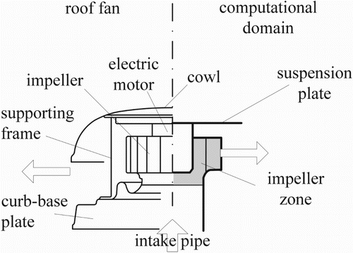
A specific characteristic with these fan designs is that the scroll housing in this instance is no longer necessary, as it generally serves the purpose of providing a weather shield above the impeller and electric motor and it regularly shaped as a simple axisymmetrical cowl (cap; Figure 1). This geometry features axisymmetrical far-field flow conditions regardless of the fan outflow direction (horizontal or vertical).

Figure 1. Roof fan.

The increase in fan pressure is calculated by averaging the CFD results for the total pressure at the fan outlet and inlet section as follows: (1) where and denote the static pressures, and are the fan outlet and inlet absolute velocities, respectively and and are the volume flow rate and air density. The outlet dynamic pressure in Equation (1) is not accounted for in roof fans according to the rules of the Air Movement and Control Association (AMCA), Eurovent (European Committee of Heating, Ventilation, Air Conditioning and Refrigeration).

The overall fan efficiency is , where is the input power for the fan, while in the CFD-based prediction of efficiency it is calculated as: (2)

The torque of the aerodynamic forces around the axis of the fan impeller rotation which result from the pressure and integrated shear stress alongside the impeller walls is defined as: (3) where is the impeller wall surface, is the normal vector and is the corresponding radius vector. The direction that coincides with the axis of rotation is designated with subscript y. The so-called disc friction torque is absorbed in as the disc surface of the impeller is included in . 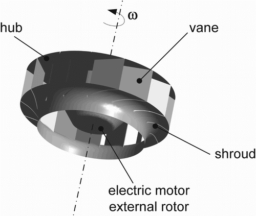The mechanical loss of power in roof fans has a negligible impact on the overall fan efficiency and is not accounted for here. Figure 2 illustrates the fully-defined fan impeller geometry.

Figure 2. Roof fan impeller.

3. Numerical modeling of the fan flow

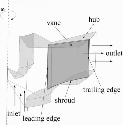
Fan flow is defined as the internal flow through the impeller passages between the impeller vanes, hub and shroud (Figure 3). The fluid is conveyed through the rotating and curved impeller channels with a rather small curvature of the vane leading edge and corners between the shroud and vanes. Deeply subsonic flow allows the constant density fluid model to be applied.

Figure 3. Fan segment.

Separation of flow in the fan channels commonly appears at off-design flow rates, contributing to the complex flow pattern and affecting the pressure distribution and hydraulic losses. In order to capture the separation, an accurate model of the shear stress is required because it significantly affects the separation.

The physical and corresponding computational domain are almost completely (surrounded) framed by fan walls and the choice of no-slip boundary conditions is straightforward:, where is the fluid velocity and is the wall velocity ( = 0 for stationary parts and  =  for the rotating impeller channels). The inlet and outlet boundaries of the computational domain are as usual somewhat arbitrary and their selection depends on the correct conditions to be prescribed along them. The inlet boundary conditions mimic the conditions inside the fan intake pipe (mass flow rate or velocity distribution along the pipe cross-section) far upstream.

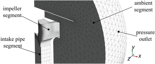
The modeled fan is almost a free impeller type and air is directly exhausted from the impeller (Figure 4). The absence of the scrolled housing (volute) which encloses the fan impeller, together with axisymmetrical conditions in the far field, allow the reduction of the computational domain to a single segment in which only one impeller vane is embedded.

Figure 4. Computational domain and boundary conditions.

The impeller outflow is not uniform and has a strong circumferential (absolute) velocity component. It decays by mixing with the ambient air. In order to account for this interaction, the outlet boundary has to be located away from the impeller exit. The computational domain is extended downstream and outflow/pressure outlet conditions can be prescribed at the outlet of this outflow zone. The flow inside the outflow zone is unsteady due to the non-uniformity of the flow at the exit from the rotating impeller. It exhibits periodicity in time as the vanes are passing by the fixed point in the stationary zone. Accurate coupling of the impeller and the outflow zone requires sliding of the impeller mesh with respect to the stationary outflow zone (Brost, Ruprecht, & Maihoefer, 2002). Coupling via a sliding mesh is highly demanding in terms of computational time and computer memory resources. The ‘frozen rotor’ coupling is more appropriate for multiple flow simulations used during the optimization process; simulating the flow for a fixed angular position of the impeller relieves the need for unsteady calculation. Except for the flow rates distant from the highest efficiency point, the frozen rotor coupling provides almost the same result as the sliding mesh (Gugau, 2002; Moradnia, Golubev, Chernoray, & Nilsson, 2014). In circumferential direction the periodic boundary conditions are prescribed and the grid structures along these periodical boundaries are identical.

Large pressure gradients require very fine grid resolution locally in the stream-wise direction in addition to the usually highly refined near-wall grid in order to resolve the velocity gradients in the thin boundary layers along the impeller vanes. An unstructured (tetrahedral) mesh is adequate for the local refinement near the vane leading edge and the vane-shroud corner areas. Testing of the CFD results using grids of different resolutions (Milas et al., 2014) showed that grid-independent results are obtained with 100,000 finite volumes inside one impeller segment of  = 325 mm impeller diameter. For simulations where the number of vanes is different from the initial condition (z = 14), the number of finite volumes was changed proportionally.

Adaptive gridding was applied to the impeller segments in order to accommodate a new generation of impeller vanes with potentially large wrap angles. In order to allow for new designs that fall outside the old computational impeller segment domain, the domain was modified if required. The corresponding segments of stationary zones were kept in the unchanged position.

A high-order discretization scheme was used and the solution was obtained by a coupled equation solver with the discretized equation maximum residuals set to 10⁻⁴.

As the fan flow is turbulent, modeling of turbulent shear stress is crucial for the calculation of fan efficiency. Numerically robust two-equation models of turbulence are good candidates for multiple simulations because they moderately expand the system of governing equations. The SST (Shear Stress Transport) turbulence model is generally preferred because it can resolve the fluid flow deep inside the viscous sublayer (Menter, Langtry, & Ruprecht, 2004). It is not dependent on wall functions that are specific for standard models in modeling the near-wall flow. Preliminary calculations with both models proved that the model provides CFD results that are as good as those of the SST model, or even slightly better.

The fan flow was simulated using the commercial CFD software Ansys (2013). The CFD model was validated by comparison with the experimental results available for the initial fan design with z = 14 flat vanes. The details of the experimental setup and experimental uncertainty are presented in Milas et al. (2014), who also illustrate that the CFD prediction follows the trend line of the experimental results. The agreement between the CFD model and the experiment was very good for a design flow rate of  = 1000 m³/h. The fan pressure and efficiency are over-predicted at high flow rates, but the maximum flow rate is very close to the experimental one.

In addition to flow simulations, this paper also includes elementary noise analysis. The major difficulty in the computation of noise is the problem scale range, as the compressible Navier–Stokes equations need to be solved for complete resolution of the acoustic field. This is not practical because of the high meshing requirements and the small time-steps required to resolve propagation of the acoustic waves. As opposed to acoustic waves, aerodynamic fluctuations take place at several orders of magnitude larger scales with comparably modest meshing and time-step requirements. In the case of far-field noise prediction, the additional requirements are large computational domains so the numerical scheme should be less dissipative and dispersive, which can deteriorate the solver stability. This is why most CFD solvers are not capable of simulating acoustic flows. To avoid direct computation of the acoustic field, several models for the prediction of noise that do not require excessive computation have been developed. Some models calculate the acoustic noise levels of fans by using only CFD results as their input.

In this paper, the Lowson (1970) model is used because it does not require excessive computation and can calculate acoustic noise levels of fans by using only CFD results. This fan noise model can be applied to low-speed fans with a tip Mach number less than 0.45. Lowson showed that the noise produced by a fan is linked directly to the aerodynamic forces exerted on the fixed and rotating vanes. The Lowson model allows the calculation of the acoustic pressure at the observer point generated by steady and unsteady forces.

4. Parametrization and optimization of the fan vane

Numerical optimization has reached a mature stage and can be successfully applied to industrial-scale engineering problems (Rao, 1996). This also applies to shape optimization, where a numerical optimizer is employed to steer the change in shape of some engineering object. Nevertheless, this requires efficient shape-representation schemes since shape optimization implies an important trade-off in modeling.

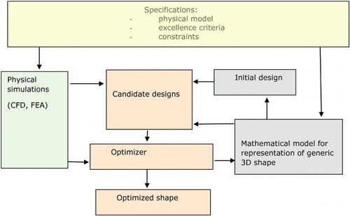
The synthesized fan shape arises based on the specifications of the excellence criteria and functionality requirements (constraints) provided by the user which jointly drive the optimizer associating this to the class of inverse problems. This is in a way a specification-based genesis of a 3D shape. In the case of this paper, the procedure is implemented using an evolutionary optimization algorithm and CFD simulation programs. The procedure is illustrated in Figure 5, which outlines the generic approach of evolutionary shape synthesis as proposed in this paper. Based on a predefined set of excellence criteria and design constraints, the optimizer algorithmically implements shape genesis using the selected mathematical entity to decode from the genotype into the corresponding phenotype and hence candidate shapes. Optimization is thereby steered by the excellence and feasibility indicators data mined from the CFD simulation results.

Figure 5. Procedure of shape optimization and design synthesis using an evolutionary optimization algorithm and CFD simulation.

Using many design variables (shape parameters) in modeling the 3D geometry of the object provides for faithful and accurate shape representation at both a local and global level. This approach is opposed to the computer-aided design (CAD) models of shape which resemble databases containing many entities (geometric primitives) along with their respective attributes (parameter values) as well as the relationships between those entities (e.g., geometric constraints). The latter translates to the overall shape consisting of many partitions with their mutual continuity and constraint relationships.

While this is adequate for CAD, it is rather inappropriate for shape optimization for several reasons. Many shape variables in the geometric model directly generate a high-dimensional search space. Consequently, the resulting large number of decision (optimization) variables leads to high computational time in optimization, possibly many local optima, slow convergence and complex simulations to evaluate excellence and constraints, etc. Moreover, the set of constraints embedded in the CAD model may be hard to impose and maintain as the shape undergoes major change.

Therefore shape optimization prefers integral shape models or at least piecewise geometric models with a moderate number of partitions and simple conditions of continuity. The number of shape parameters (decision variables in optimization) should be just sufficient for the required local and global modeling capacity.

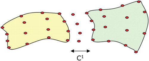
Using partitioned shape representations in this context implies adaptive chaining of piecewise parametric curves and surfaces. In this case, low-degree patches are networked mutually with an adaptive subdivision of the object surface, thus preserving the locality of each patch. The typically necessary C¹ continuity at the interfaces (Figure 6) among the patches should be accomplished by generating extra control points without increasing the number of design variables or in some cases by applying Lagrange functions. Within the framework of this paper, C¹ continuity implies continuity of the function (parametric surface) and its first derivative. This imposes continuity of slope between the partitions which is commonly sufficient in engineering shape optimization. While the Lagrangian can be used to enforce continuity requirements, it is frequently convenient to interpolate additional control points at the patch edges as the respective two end control points (Figure 6) are responsible for the end slope. The decomposition of the overall surface into patches should be carried out such that a minimum number of parameters represent the shape of the overall surface with sufficient accuracy and moderate capability for local and global change of shape. Nevertheless, any parameterization of 3D shapes acts as a loose geometric data-set compression, and some representation capacity is always sacrificed.

Figure 6. C1 continuity patch interfaces.

The integration of piecewise patches is automatically implemented by applying piecewise polynomial B-spline and rational NURBS (Non-uniform rational B-spline) surfaces. These exhibit local control of shape as each control point affects only a few segments in its vicinity, as defined by the corresponding knot vector. This is a geometric model that is well suited to shape optimization since the optimizer can invoke isolated local changes of shape in the object.

The computational workflow needed to implement the procedure (Figure 5) should be a distributed system, encapsulating existing CAD and CFD software, coupled with the evolutionary numerical optimization. The numerical coupling needs to include both the process executions and their mutual synchronization, as well as data flows between the individual applications.

4.1. Optimization

The engineering object considered in this paper is the roof fan according to specifications listed later. It will be optimized for energy conversion efficiency under given operational conditions. The problem is a hybrid optimization case, as some of the variables are discrete (number of vanes) while other are continuous (rotational speed, shape parameters defining the shape of the vanes). The vanes were modeled as fully generic 3D shapes using computational geometry primitives (e.g., B-spline surfaces) rather than using specific models based on few physical parameters such as vane angles.

The design objectives are usually related to some tangible physical criteria such as total mass or selected performance benchmarks at the nominal operating point. Nevertheless, such objectives may lead to suboptimal performance in the optimized engineering object in terms of the overall lifetime due to the fact that the object will not be operating at the nominal regime throughout its operational ‘future’, but will instead be subjected to many different regimes. The shape optimized for the nominal point need not imply (and usually does not) maximum excellence for the overall life cycle of the object.

Shape optimization needs to be steered by realistic life-cycle-based benchmarks of performance excellence, which require the implementation of coupled financial and engineering modeling. Such an approach was implemented in Vučina, Lozina, & Pehnec (2010) using the net present value (NPV) or internal rate of return (IRR) metrics.

In this paper the somewhat simplified approach of robust shape optimization was followed. It does not involve coupled financial–physical modeling, but instead defines a mix of operating regimes for which the respective engineering optimality is defined, which is an approach fully justified for this case. This means that a distribution of environmental and operating conditions for the roof fan is defined (for example a distribution of flow rates), based on which a representative sample is generated for the numerical optimization. The optimizer uses the combined excellence across this distribution of regimes to assess the optimality of each candidate shape. A detailed description of these cases accompanies the examples provided later.

In the case of robust optimization, the objective is not maximum efficiency but maximizing the mean value and minimizing the standard deviation. In the core of this paper, the optimization suite modeFRONTIER (Derakhshan, Pourmahdavi, Abdolahnejad, Reihani, & Ojaghi, 2013) was used as the optimization integrator. To efficiently compute the mean and standard deviation, a Latin hypercube set of samples was used in combination with polynomial chaos expansion (ESTECO, 2013) instead of classical estimators such as Monte Carlo.

4.2. Parametrization

Given the fact that fully generic 3D shape modeling, complex 3D CFD simulations, and robust optimization are combined, a high computational cost for the resultant numerical workflow can be expected. Efficient shape parameterization is therefore crucial for the optimization of the geometry.

In order to alleviate some of the computational complexity, a partitioned model of the geometry based on CAD standards is abandoned due to its complexity. Namely, CAD models involve databases with individual geometric primitives and their mutual relationships (geometric constraints, etc.), i.e., they proceed with the logic of fully-partitioned geometry.

The optimization variables in the case of such partitioned representations based on parametric CAD feature-based models can be used for some of the parameters, such as features of individual elementary solid modeling primitives, control points of 2D curves, operators generating 3D shapes from 2D curves, and positions and orientations of individual elements, etc. (for example, see Dai, Gu, Zhao, & Guo, 2005; Hardee et al., 1999).

Instead, the approach here is to apply integral geometric parameterizations which extend across the entire object. This approach enables the workflow to be computationally more efficient, since the changes in shape are related to the integral shape model. There is no need to verify whether interference with other objects in the CAD database has occurred or whether any constraints which relate to different entities in the CAD model have been compromised. Moreover, the examples will prove that the parameterizations are also flexible enough and provide sufficient degrees of freedom to represent the necessary changes in shape. The NURBS-based (Bohm, Farin, & Kahmann, 1984; Farin, 1993) integral shape parameterization is also scalable, as the size of control points grid and the basic polynomials degree can be varied. This allows an optimal compromise to be reached between the geometric modeling capacity and the search space dimensionality. Modest dimensionality of the design space should be maintained while simultaneously providing sufficient geometric modeling freedom for the optimizer to impose any appropriate change in local and global shape.

Representation of a complex 3D shape based on a single polynomial surface may require high-degree polynomials, which in addition to oscillatory behavior lack local control. Combination of these properties is likely to introduce unnecessary numerical complexity; therefore, the only viable option is chained low-degree d surfaces, which provide local control and continuity resulting in numerically-efficient shape parameterization. B-spline surfaces are applied in the examples, defined recursively as: (4) with (5) and (6)

The surface in Equations (4) to (6) features the local control property since the support range of an individual shape function N_i,j(t) is given by its non-zero values only in the interval t_i, t_{i + j + 1}, while being zero for t < t_i and t ≥ t_{i + j + 1}, which applies to both component directions of the surface. Consequently, the surface is locally formed exclusively by a few neighboring control points, Q_ij. In both component directions, the first and last (d + 1) knots are set to 0 and 1 respectively in order for the surface to pass through the end curves. The blending functions N possess the properties of non-negativity, local support and partition of unity. The shape of the B-spline surface can be adjusted by moving the control points and modifying the knot vectors.

4.3. Optimization and parameterization of the centrifugal fan

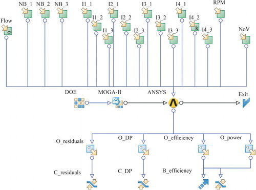
In this paper, the multi-objective optimization MOGA-II (improved multi-objective genetic algorithm) (Derakhshan et al., 2013) was used along with an ANSYS (2013) CFD simulation to generate the Pareto front for a-posteriori decision-making. The control points of the B-spline surface, the number of vanes and the rotational speed were used as optimization variables. The CFD outputs including the pressure difference, efficiency and residuals were used to evaluate the objectives and constraints.

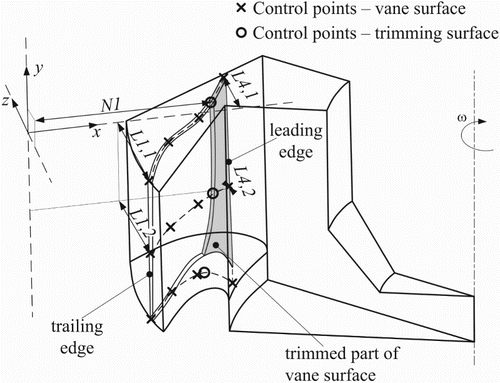
A B-spline surface which describes the vane shape subjected to optimization is constructed using a 4×3 grid of control points (Figure 7), where only three points are for clarity. To specify individual control points, each is designated as L_i,j, where i represents the column number and j represents the row number. Only the distance of individual control points from the x-y plane is taken to be the optimization variable in order to reduce the number of variables. To further improve the convergence rate, the point L_4,2 is fixed so that the ‘rigid-body motion’ of the vanes is prevented. An additional three variables designated as N_i are used for modifying the meridian projection of the vane's leading edge (trimming; Figure 7).

Figure 7. Parameterization of vane.

To completely define the computational domain of a fan segment one must define the individual vane shape, the number of vanes and the hub and shroud, which are not subject to optimization in this paper. While the vane shape is parameterized using B-spline, the number of vanes is realized by simply expanding the computational domain symmetrically with the rotation of existing boundaries (Figure 8). This type of parameterization of the computational domain in relation to the number of vanes is called parameterization with rigid periodic boundaries in this paper. The boundaries are described as ‘rigid’ because they remain rigid for any number of vanes, as opposed to flexible boundaries (Figure 9).

Figure 8. Parameterization of domain with rigid periodic boundaries.

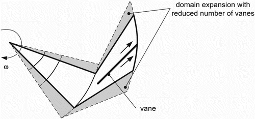
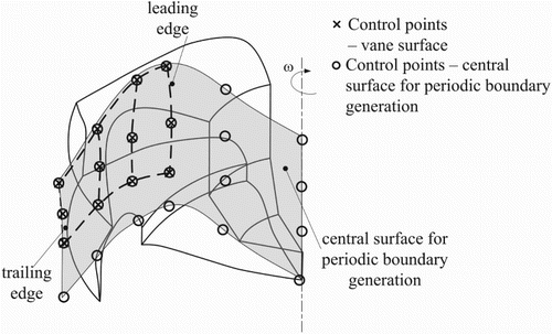
Figure 9. Central surface for the generation of periodic boundaries for parameterization with flexible periodic boundaries.

The allowable range of values for the L_i,j variables has to be constrained in the case of the parameterization of the domain with rigid periodic boundaries; the ranges were constrained so that vanes do not break through the nearby periodic boundaries.

To avoid the need for constraints that restrict the shape of the vanes, another type of domain parameterization is developed. Initially a kind of central surface is generated using the control points of the vane surface and the periodic boundaries are generated by symmetric rotation in both directions (Figure 9). While the vane surface has 3×4 control points, the surface for generating periodic boundaries has 4×6 control points. From 24 control points belonging to a surface for generating periodic boundaries, only 12 control points have common coordinates in space. As a result there will be no perfect match between the periodic boundaries and the vane surface.

Convergence criteria must be applied during the shape optimization procedure in order to stop the process once an optimal or near-optimal solution is obtained. If the improvement in efficiency is not significant during several consecutive generations, the process is terminated. In previous study (Milas, Vučina & Marinić-Kragić, 2014), about 1,000 iterations were required to reach the optimal solution for the 2D shape optimization case, while in this paper for the 3D shape optimization cases 15,000 iterations were usually required. In this paper, the genetic algorithm (Goldberg, 1989) was used to achieve a near-optimal solution and the simplex method was used to achieve the final optimal solution in order to increase the convergence speed.

Computational workflows can be assembled for complex physical optimization assignments (Vučina, Lozina, & Pehnec, 2012; Vučina, Milas, & Pehnec, 2012). 3D-shape optimization requires multiple shape variables to be included in the computational workflow (Figure 10). The workflow schematically represents process flows and data flow between the evolutionary optimizer and implemented 3D parametric shape modeler and a CFD simulator.

Figure 10. Shape optimization variables in computational workflow.

Note: ANSYSWB1 = CFD simulation code; B_efficiency = optimization objective, max η; C_residuals = design constraint, CFD residuals; C_DP = design constraint, Δp_f; DOE = design of experimental module for the creation of the initial population; Exit = end of single simulation process; Flow = input, statistical distribution of flow rates; li_j = parameter specified in Figure 7; MOGA-II = optimizer for multi-objective optimization based on a genetic algorithm; NB_i = parameter specified in Figure 7; NoV = number of vanes; O_DP = result of CFD simulation code, fan pressure Δp_f; O_efficiency = result of CFD simulation code, efficiency η; O_residuals = result of CFD simulation code, equation solver residual; RPM = rotation speed.

4.4. Single-point optimization procedure

The first implemented optimization procedure is single-point optimization. The optimization objective is the maximization of the efficiency of the nominal design flow. The total fan pressure Δp_t has been constrained to 80 Pa with allowable difference of 10 Pa at a design point of 1000 m³/h. The discretized equation residuals are monitored and designs that do not achieve 10⁻⁴ are considered infeasible. These categories of infeasible designs consist of highly curved unusual shapes and no optimal solution is expected to belong to this group.

4.5. Robust optimization procedure

For the robust optimization procedure, the optimization objective is the maximization of the mean efficiency for a given statistical flow range, which is described as having a normal distribution with a mean value set to 1000 m³/h and a standard deviation of 150 m³/h. The total fan pressure at the flow rate of 1000 m³/h is constrained, as with the single-point optimization procedure, meaning that every design evaluation includes the simulation for 1000 m³/h, while the flow rate for other simulations is set by random patterns derived from a given statistical distribution. As before the residuals are monitored and designs are marked as unfeasible if the preset criteria are not met.

4.6. Decision-making using noise analysis

One more possibility is to conduct a multi-objective optimization using noise minimization as the second objective. Noise can be described by the distribution of sound pressure levels over the relevant frequency range, but an overall sound pressure level measurement is not a good indication of noise intensity because the ear is not equally perceptive to all frequencies. To represent noise as the ear would perceive it, a system of weighting networks is applied to the sound pressure levels at various frequencies. The most commonly used standard for noise in the industry is the ‘A’ weighting (Sound Research Laboratories, 2002) as a good agreement between weighted sound levels and the subjective responses. The high computational requirements for the resolution of the acoustic field make the direct methods impractical for optimization purposes, so more elementary methods must be applied here. This paper uses the Lowson overall noise sound pressure level as the objective for the minimization of noise. Excessive computation is thereby avoided since only stationary regime CFD results are required for this model. The predictions of noise levels obtained by this method are good for comparative analysis, while the absolute values of the predicted noise levels are not expected to be accurate, making it suitable for preliminary analysis and optimization cases.

5. Results

The conducted optimization cases for various sets of constraints are presented in Table 1. Case 1 is the reference case, with vanes optimized as single curved (or 2D) surfaces (Milas et al., 2014). For comparison with other designs, the results for the 2D optimized fan for a single flow rate designated Case 1 are presented first. The optimization variables were the 2D shape parameters of the vanes while the number of vanes and rotational speed were constant and the single-point optimization procedure was applied for a design flow rate of 1000 m³/h. Peak efficiency was reached at the design flow rate and amounts to 50.6%, while the pressure is 83.5 Pa.

Table 1. Conducted optimization cases for various set of constraints.

Case	Setup	Optimization goals	Free parameters determined by optimization
1	Single flow rate, z = 14, ω =103	Max η	Vane 2D shape
2	Single flow rate, z = 14, ω =103	Max η	Vane 3D shape
3	Range of flows, z = 14, ω = 103	Max mean η	Vane 3D shape
4	Single flow rate	Max η	Vane 3D shape, z, ω
5	Range of flows	Max mean η	Vane 3D shape, z, ω

Note: η_max = (maximum) peak efficiency; ω = impeller rotational speed (rad/s); z = number of impeller vanes.

The next two cases are scenarios with only the vane shape as the optimization variable. The remaining two cases consider the number of vanes and operational speed as variables while a different optimization procedure is applied. Single-point optimization was applied to Cases 2 and 4, where the design goal is the maximization of the efficiency of the design flow rate. The robust optimization procedure, where the optimization objective is the maximization of the mean efficiency for a given statistical flow range, was used in Case 3 and Case 5.

5.1. Sensitivity to initial population

Optimization cases with only the vane shape as the optimization variable achieve convergence to global optimum easily by initializing the population with the Sobol procedure (ESTECO, 2013) using 100 designs. The particular genetic algorithm for optimization was MOGA-II, and convergence was achieved within 40 generations, after which only negligible improvement occurred. For cases where the number of vanes and speed of rotation are the optimization variables, convergence to global optimum proved difficult to achieve. When the optimization procedure was applied to Case 4, the converged solution was somewhat different depending on the population initialization. At first, optimization was conducted using a Sobol population initialization with 100 designs, and the converged solution was obtained after 50 generations with the resulting efficiency of 55.5% (Figure 11).

Figure 11. Optimization of Case 4 using Sobol population initialization with 100 designs.

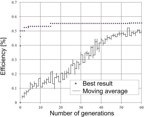
To confirm the result as the global optimal solution, optimization was conducted using Sobol population initialization with 200 designs, and this time the converged solution was obtained after 55 generations with a resulting efficiency for this optimization of 56.5%. This means that the former initialization with a smaller initial population converged to a local minimum and the latter is likely to be the global optimal solution. This was confirmed when the optimal efficiency remained the same for the latter optimization with larger population sizes. With this conclusion, the remaining optimizations were conducted using Sobol, population initialization with at least 200 designs. In both cases little improvement was made by applying the Nelder–Mead simplex method for local optimization after the global MOGA-II optimization was converged. As the starting simplex for the Nelder–Mead method, N + 1 best design points were used where N is the number of variables. Local optimization usually converged within 300 design evaluations.

5.2. Sensitivity to periodic boundary parameterization analysis

There should be no difference for the solution for the parameterization of the domain between the usage of rigid periodic boundaries and flexible periodic boundaries with the same vane geometry, number of vanes and operating speed. To empirically confirm this assertion, a flat vane was simulated for both domain parameterizations, which yielded the same results for efficiency and pressure. Parameterization of the domain with flexible periodic boundaries allows more freedom for the shape of the vanes since they are not restricted within the confines of rigid boundaries. The next step was to see whether the resulting optimal solution was any different now that more freedom of shape synthesis was available.

Case 2 was optimized using both domain parameterizations and yielded the same result in both cases. This proved empirically that the shape of the periodic boundary does not affect the result of the simulation. The resulting peak efficiency is 56.9%, which is 14% higher compared to the flat vane fan design and 6% compared to the 2D optimized vane design in Case 1.

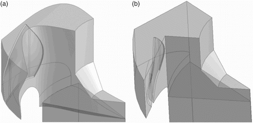
The next analysis was of Case 4, where the optimization procedure was conducted on both domain parameterizations and resulted in two geometrically different solutions with different numbers of vanes. While different in terms of input variables, the peak efficiency of both solutions is nearly equal and amounts to 57.2% at the design flow rate. The two different solutions for the Case 4 optimizations are different not only in shape but also in the number of vanes. The geometry of Case 4 optimized a vane shape by using a rigid domain that converged to 13 vanes compared to one with 9 vanes optimized using the flexible domain with noise analysis.

It is not unexpected that different shapes can result in similar performance; from a mathematical perspective, highly-nonlinear models frequently possess local optima, as the multi-dimensional geometric design space maps into the single (or low) dimensional criteria space. Also from an engineering perspective, it can be observed that different shapes and designs exist based on different sets of criteria and requirements. The diversity in nature itself but also in engineering designs can loosely be viewed as local optima resulting from different settings or different yet similarly successful approaches to the same problem.

At this point only the shape of Case 4 with flexible domain parameterization is discussed. A view of the solution in the case obtained by using flexible periodic boundaries is given in Figure 12(a), while Figure 12(b) shows that the geometry of the solution obtained by this parameterization cannot be replicated using the model with rigid periodic boundaries. Another important conclusion is that for single-point optimization, the solution does not have to be unique, which implies that another criterion must be introduced to obtain a unique solution, or that some other optimization objective must be adopted. Another possible method of solving the uniqueness problem considered in this paper is the application of a robust optimization procedure and a multispeed optimization procedure.

Figure 12. Perspective view of Case 4 for solution with: (a) flexible periodic boundaries and (b) rigid periodic boundaries.

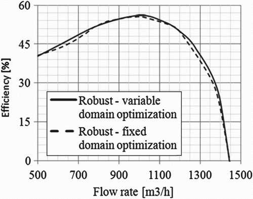
Since each robust optimization consumes far more computational resources than single-point optimization, Case 3 was skipped for analysis of the sensitivity on the domain parameterization. Only the Case 5 robust optimization was analyzed. This optimization resulted in two geometrically different solutions with different numbers of vanes, but unlike the analysis of Case 2, with small but noticeable differences in objective value, the mean value of efficiency for the case with rigid periodic boundaries for the optimal solution was 54.8% while using variable boundaries it amounted to 55.2%.The efficiency characteristics of fans designed using the robust optimization procedure obtained using flexible periodic boundaries and rigid periodic boundaries are almost identical (Figure 13).

Figure 13. Efficiency characteristics of fan designed using he robust optimization procedure obtained for a model using flexible periodic boundaries and rigid periodic boundaries.

5.3. Robust optimization and comparison with single point

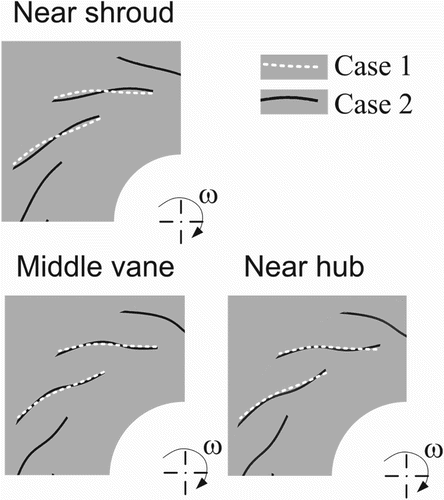
The first case is the 2D vane shape, which is used for reference. The next two are the 3D vane shape optimization cases with a constant number of vanes and rotational speed but with different objective functions, as discussed earlier. The resulting vane optimized for a single flow rate is of a double curved type (Figure 14). In the stream-wise direction (looking from the leading to trailing vane edge) its shape resembles the 2D optimized vane shape for Case 1. The vane outlet angle is higher than in Case 2 and ranges from 40° near the shroud to 28° near the hub. In Case 2, the shape is straight at the inlet part of the vane profile then gradually turns into a convex one. The vane outlet angle is lowered to about 28°, being smaller than the corresponding angle of the flat vane (45°) or any of the 2D optimized vanes (∼30°). The vane is slightly convex in the span-wise direction (from hub to shroud).

Figure 14. Case 2 optimized vane profile (shroud, midspan and hub) compared to Case 1.

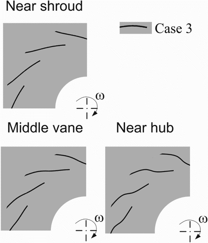
The effect of the robust optimization of the vane in Case 3 is as expected regarding fan performance; the efficiency curve is less steep and the maximum flow rate has again increased to 1400 m³/h, with higher values of efficiency maintained at overflow rates, (Figure 16). The efficiency is a bit lower than for the single flow rate optimization. The stream-wise vane profile is different from those of Cases 1 and 2, with less curvature in the profile. The vane outlet angle is now lower, ranging from 36° near the hub to 25° close to the shroud (Figure 15).

Figure 15 Fan performance for Case 2 (single point) and Case 3 (robust) compared with Case 1.

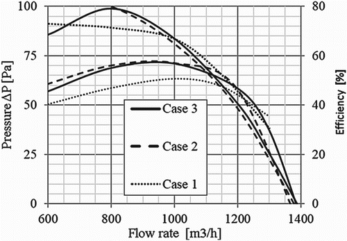
The Δp_f-V performance curve is steeper than the one for the flat vane design. Its efficiency exceeds that of the flat vane design and all of the 2D optimized vane designs in the range of flows from 600 to 1200 m³/h (Figure 16).

Figure 16. Case 3 optimized vane profile (shroud, midspan and hub).

The next two optimization cases are 3D vane shape optimization with the number of vanes and rotational speed as additional variables. The single-point optimized vane of Case 4 is backward curved and the vane outlet angle is almost constant (32°) along the trailing edge (Figure 17). In the stream-wise direction, the vane is uniformly curved and cambered from the suction to the pressure side. Close to the hub, the vane profile turns into a straight one. The vane is slightly convex in the span-wise direction at the inlet but turns into a V shape towards the impeller outlet (Figure 17).

Figure 17. Comparison of Case 4 with Case 4b optimization.

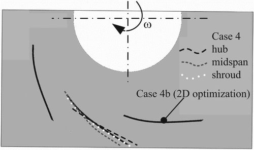
It is interesting to compare the shape of the 2D vane optimized with the same design freedom (number of vanes and rotational speed) as in Case 4. This case is designated as Case 4b. The 2D vane profile looks like the average of the 3D vane profiles at various sections from hub to shroud (Figure 18). While the peak efficiency of Case 4 is 57.2% as specified earlier, the efficiency of the 2D optimized fan (Case 4b) exhibits a lower peak efficiency of 55.5%. This indicates that the 3D vane shape moderately improves the fan efficiency; the absolute increase in peak efficiency is 1.7%.

Figure 18. Fan characteristics for optimized impeller vanes for Case 4.

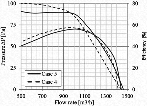
The fan pressure–capacity characteristic for Case 4 is as steep as the one for Case 2 (Figures 16 and 18). There is no significant gain in the fan efficiency; nevertheless, this is accomplished with a reduced number of impeller vanes (z = 9) in comparison with Cases 1 to 3. The variation of the rotational speed that was allowed during optimization resulted in a slightly higher value of ω = 114 rad/s for which the design-prescribed fan pressure of 80 ± 10 Pa was achieved. The peak efficiency of  = 57% was obtained for the design flow rate of  = 1000 m³/h, changing very little in the range of flow rates between 800 and 1100 m³/h.

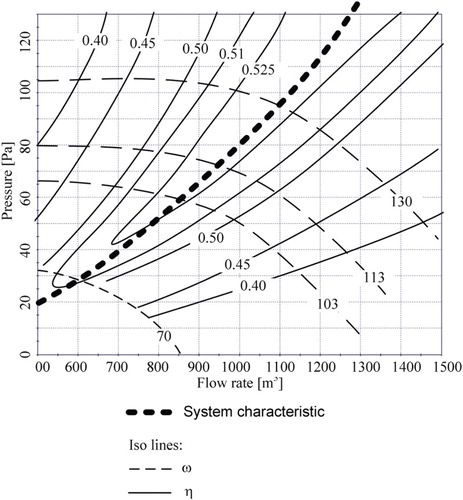
The effect of optimization with respect to the rotational speed is verified by the ‘hill diagram’ with lines representing constant fan efficiency (Figure 19), indicating that for the optimized speed of 114 s⁻¹ and design flow rate of 1000 m³/h, the corresponding value of efficiency (57%) is close to the top value for the optimized 3D vane shape.

Figure 19. Iso lines of efficiency and rotational speed for Case 4.

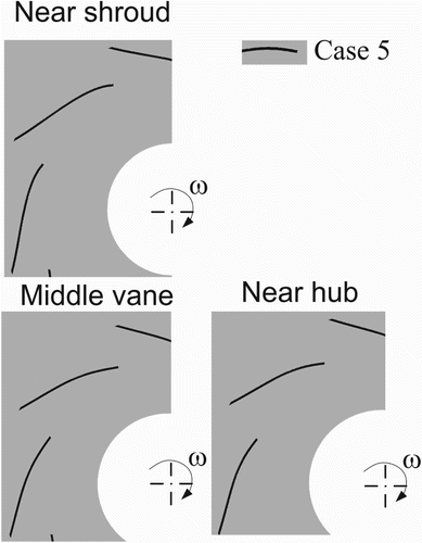
Regarding the vane shape, the outlet angle for robust optimization (Case 5) is almost constant and amounts to 32°, which is same angle as in Case 4. Robust optimization for the range of flows in Case 5 provides maximum efficiency at 115 s⁻¹, almost the same rotational speed as in Case 4 but using a smaller number of impeller vanes (z = 8). The vane shape obtained by optimization is less curved in the span-wise direction (Figure 20) and there is no V-shaped trough at the vane outlet.

Figure 20. Case 5 vane profile (shroud, midspan and hub).

Since some S-shaped curvature oscillations are apparent in part of the optimization results (S-shaped vanes), the following considerations provide potential arguments for the optimization methods being a possible cause of these results. Slight curvature oscillations or local shape variations can in many cases be caused by roots embedded in numerical models. It should be kept in mind that the shape optimizer steers a large multitude of control points and consequently modifies both local and global shape. Many generations of evolutionary optimization are needed for convergence to the optimum design, especially knowing that convergence of the evolutionary algorithms, once they arrive in the vicinity of the solution in the design space, may be slow. This is especially true if the optimizer is launched from arbitrary or ‘distant’ initial designs. On the other hand, a limited number of generations are commonly applied. Another factor to be considered is the fact that the sensitivity of the excellence function (related to the performance of the vane) with respect to the vane shape (set of control points) may be very low, potentially leading to poor convergence rates in mature generations.

Different numerical operators could be applied to relieve the local shape variations. As an example, geometric filters based on local curvature can be applied to ‘stretch’ and smoothen the local shape. Alternatively, multi-stage optimization can be applied with fewer shape variables initially then successively introducing more shape parameters starting from the previously attained solutions. In such cases, the transfer of the current shape from stage to stage can be implemented by fitting higher-dimensional parametric surfaces onto the lower-dimensional ones. While these interventions would be accommodated in a real industrial scenario, this paper demonstrates the reality of ‘pure’ numerical shape optimization without such processing. Obviously, these numerical problems are not present with traditional shape models based on physical entities employed as shape variables (i.e., lengths, angles, etc.) since they offer far less geometric generality.

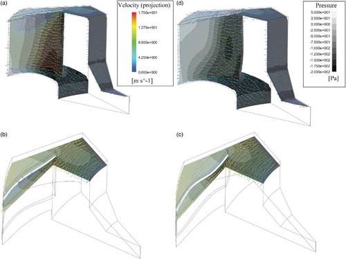
S-shaped vanes can be found in highly efficient centrifugal compressors but are uncommon in fan design (Guzovic, Baburic, & Matijasevic, 2005). The effect of 3D optimization, resulting in S-shaped vanes, is elucidated with the analysis of flow patterns in 2D and 3D optimized fan vanes. The 3D optimized vane in Case 2 provides a bit of gain in the fan efficiency compared to the less S-shaped 2D vane. It is helpful to note again that the efficiency of the optimized fan in all cases is low partly due to neglected kinetic energy at the fan outlet, which is standard practice in the AMCA and Eurovent guidelines for the pressure of fans without outlet ducts. The gain in efficiency can be explained by Figure 21(a) and (b), which illustrates a large separation region close to the hub on the vane suction side for the 2D optimized vane in Case 1; the recirculation is evident in the perspective view of the surface offset 1 mm from the vane suction side. By 3D optimization, this recirculation is remedied and thereby contributes to the higher peak efficiency (Figure 21(c) and (d)).

Figure 21. Flow patterns for V = 1000 m³/h: (a) separation of flow in upper part of impeller channel, (b) recirculation region along vane suction side, (c) flow pattern for optimized 3D vane in Case 2, and (d) sectional view of optimized 3D vane (suction side) without separation.

The 3D optimized vanes have a variable lean angle from hub to shroud. The impeller vane lean affects the velocity at the impeller outlet and the secondary flows in the impeller channel. The flow at the impeller outlet is more uniform. The introduction of a lean suppresses the secondary flows and contributes to lower secondary losses and increased efficiency.

5.4. Noise analysis as an added selection criterion for Case 4

When multiple solutions with equal objective values exist in single-point optimization, different options may be considered. One possibility is to conduct multi-objective optimization using noise minimization as a second objective. Here, noise analysis is considered as the second-order criterion towards deciding which of the multiple solutions should be optimal in this case. In the analysis of Case 4, two solutions with equal values of the optimization objective have appeared but they have different geometry, numbers of vanes and rotational speeds. It is expected that since the fan designs are different in terms of the input variables, the produced noise will not be equal.

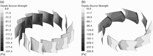
Ffowcs-Williams and Hawkings (1969) present the expressions for the density field radiated by turbulence in the presence of arbitrarily moving surfaces. The dipole source strength derived from their equations, which is the most influential noise source among surface sources, is shown in Figure 22 for both cases. It can be seen that the extreme values of source strength are larger in the case optimized with flexible domain parameterization. The Lowson overall noise sound pressure level with an observer at 0.5 m distance for the case optimized using the rigid domain amounts to 29 dB, while for the case optimized using the flexible domain parameterization it amounts to 35 dB. With this result in mind it can be concluded that rigid domain parameterization is optimal for Case 4.

Figure 22. Dipole source strength derived (Ffowcs-Williams & Hawkings, 1969) for Case 4 optimized in (a) a rigid domain parameterization and (b) a flexible domain parameterization.

The final optimization case in this paper is a preliminary multi-objective optimization similar to Case 4 with the additional objective of minimizing the overall noise sound pressure level. The optimization is conducted for 30 generations with MOGA-II optimization and a population size of 100 designs. Figure 23 illustrates the Pareto front of minimal noise vs maximal efficiency. The noise level is scaled so that the values are of the same order of magnitude as the efficiency, otherwise the Pareto front may not be formed adequately.

Figure 23. Pareto front obtained by multi-objective optimization for maximum efficiency and minimal noise.

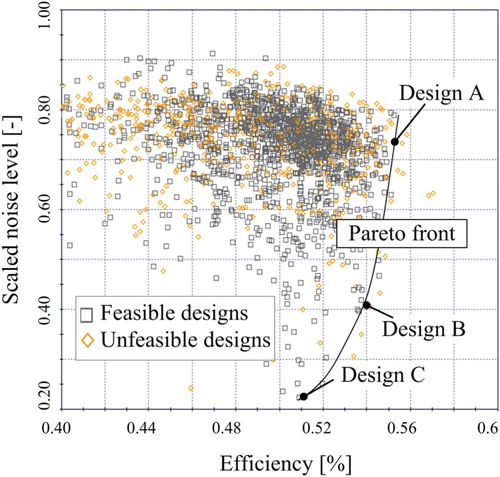
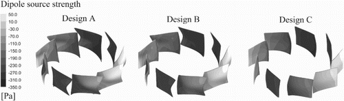
Figure 24. Dipole source strength isometric view of selected designs on the Pareto front from multi-objective optimization.

Three designs are selected from the Pareto front to illustrate the impact of the additional objective on the resulting vane shape. Design A is on the efficiency side of the Pareto front with a 55% efficiency value while the fan generates an overall noise of 39 dB. Design B is located approximately in the middle of the Pareto front with a performance of  = 54% and a noise level amounting to 29 dB. Design C generates the least noise (20 dB) but with a noticeable drop in efficiency ( = 51%). The efficiency drop can be explained in the same manner as in Case 1, as here similar local zones of flow separation exist. Note that the results of the overall noise levels are good only for comparative analysis while absolute values are usually not accurate. Figure 24 illustrates the selected designs from the Pareto front with dipole sources strength; the extreme values of source strength are greater for vane shapes that generate more noise. As shown in Figure 24, the noise reduction has a local shape smoothening effect, i.e., the smoother vane shape provides lower acoustic emissions.

5.5. Summary of results

The paper goes further than just applying CFD and optimization methods, as particular codes are not of any importance here. The problem of design synthesis of fans and pumps was dealt with in Derakhshan et al. (2013) using various combinations of design variables and procedures. Most vane shape optimization approaches in other papers have only used physical features as design parameters. It is common practice to use vane angles at the leading and trailing edges, curvatures and inlet and outlet edge positions as design parameters. While adopting physical features as design parameters offers a naturally logical and practical choice, it is inadequate for generic shape optimization; therefore, the developed shape parameterization is superior regarding modeling freedom. Using parametric surfaces to develop a fully generic 3D freedom of shape for a centrifugal fan vane is the primary contribution of the paper. Furthermore, the same parametric surface can be used for the definition of both the vane shape and the periodic boundaries, allowing for even greater shape freedom compared to rigid periodic boundaries. Regarding the optimization procedure, the contributions include the application of a memetic algorithm and the combination of MOGA-II and the Nelder–Mead simplex method for achieving faster convergence. Finally, the paper deals with resolving equally excellent shapes by introducing a multi-objective criteria optimization case with the application of elementary noise analysis to the CFD results.

An application of completely generic modeling of the vane shape allows the optimizer to generate practically arbitrary geometric shapes and is able to represent a global shape as well as potential local adaptations. Every generated shape is subsequently evaluated using a CFD simulation operating in the numerical workflow, controlled by middle-ware programs for data mining and synchronization of the numerical workflow. CFD simulation codes and an optimizer implementing the described numerical procedures and physical models can be arbitrarily chosen as an alternative to commercial off-the-shelf software and subsequently replace the current simulation node (Figure 10) shown in the workflow.

6. Conclusion

The developed workflow demonstrates that a numerical procedure able to autonomously synthesize centrifugal fans with a generic 3D vane shape is truly possible. This procedure can accommodate multiple cases of optimization enabling customized and individualized fan design for specific working environments according to the selected excellence criteria. The objective realized cases are maximum efficiency, overall energy consumption in multi-regime operation distributions, and minimization of fan noise for the multi-objective case. The 3D shape has shown the potential to reduce flow losses caused by the separation of flow that cannot be eliminated using 2D shape optimization only. The corresponding increase in peak efficiency is Δη = 5–6% with slightly greater efficiency achievable in optimization by including the number of vanes and the rotational speed as optimization parameters.

The most promising vane shape is obtained via robust optimization where the additional optimization variables are the number of vanes and the rotational speed, together with the 3D vane shape geometry. The case displays less curvature compared to other designs and has the least number of vanes such that fan fabrication can be implemented more easily. It has been shown that in some cases no single optimal solution exists, hence another optimization objective can be implemented, in this case noise minimization. Further promising cases involve multi-objective optimization for potentially great noise reduction with only a small decrease in efficiency. Reduction in fan noise is for some designs followed by less curvature, again making them easier to manufacture. In all optimization cases the vane thickness as well as the impeller meridional section were kept constant, leaving space for further improvement.

The current study shows encouraging results and represents a foundation for further study. The planned future work will include 3D CFD stationary regime simulations and search for possible improvement as the off design-point performance curve can possibly achieve better agreement with experiments. Since a stationary regime simulation only offers elementary noise analysis, future work will consider unsteady simulations and flow-decoupled acoustic wave simulations for more comprehensive noise analysis.

The complex shapes of the optimized vanes invite experimental validation, particularly regarding the effect of the vane camber in the direction from hub to shroud. Future work will also consider manufacturing-related objectives, as some obtained shapes with complex double-curved 3D vanes only show a small improvement in efficiency compared to relatively simple shapes. There is still room for achieving higher efficiencies because some geometric features of the centrifugal fan have been left out in this paper. Additional degrees of freedom will be included such as varying the thickness and varying the meridional section of the impeller. The multi-objective case conducted here is only a preliminary one; the planned future work will include general multi-objective optimization with more comprehensive noise minimization as the secondary objective.

Disclosure statement

No potential conflict of interest was reported by the authors.

Funding

This work was supported by the Croatian Science Foundation [grant number IP-2014-09-6130].

ORCID

Ivo Marinić-Kragić http://orcid.org/0000-0002-9680-6193

References

- Adnot, J., Kemna, R., & Hitchin, R. (2012). Technical analysis of ventilation systems for non-residential and collective residential applications (Final Report Task 5). VHK. Retrieved from http://www.ecohvac.eu
- Ansys, Inc. (2013). ANSYS CFD (Version 14.5) [computer software]. Retrieved from http://www.ansys.com.
- Arora, J. (1989). Introduction to optimum design. New York: McGraw-Hill.
- Bertoldi, P., & Atanasiu, B. (2009). Electricity consumption and efficiency trends in EU (Status report). JRC Scientific and technical reports. Retrieved from http://iet.jrc.ec.europa.eu/.
- Bohm, W., Farin, G., & Kahmann, J. (1984). A survey of curve and surface methods in CAGD. Computer Aided Geometric Design, 1, 1–60. doi:10.1016/0167-8396(84)90003-7
- Brost, V., Ruprecht, A., & Maihoefer, M. (2002). Rotor stator interactions in a axial turbine, A comparison of transient and steady state frozen simulation. Inst. Fluid Mechanics and Hydraulic Machinery, Uni. Stuttgart, Germany.
- Chau, K. W., & Wu, C. L. (2010). A hybrid model coupled with singular spectrum analysis for daily rainfall prediction. Journal of Hydroinformatics, 12, 458–473. 10.2166/hydro.2010.032 doi: 10.2166/hydro.2010.032
- Dai, L., Gu, Y., Zhao, G., & Guo, Y. (2005). Structural shape optimization based on parametric dimension-driving and CAD software integration. 6th World Congress on Structural and Multidisciplinary Optimization, 1–8, Rio de Janeiro, Brazil.
- Deb, K., & Goel, T. (2002). Multi-objective evolutionary algorithms for engineering shape design (KanGAL report). Indian Institute of Technology Kanpur.
- Derakhshan, S., Pourmahdavi, M., Abdolahnejad, E., Reihani, A., & Ojaghi, A. (2013). Numerical shape optimization of a centrifugal pump impeller using artificial bee colony algorithm. Computers & Fluids, 81, 145–151. 10.1016/j.compfluid.2013.04.018 doi: 10.1016/j.compfluid.2013.04.018
- ESTECO. (2013). modeFRONTIER.(Version 4.5) [computer software]. Retrieved from htttp://doi:www.esteco.com
- Farin, G. (1993). Curves and surfaces for computer aided geometric design. San Diego: Academic Press.
- Ffowcs-Williams, J. E., & Hawkings, D. L. (1969). Sound Generation by Turbulence and Surfaces in Arbitrary Motion. Proc. Roy. Soc. London, 264, 321–342. doi:10.1098/rsta.1969.0031
- Goldberg, D. E. (1989). Genetic algorithms in search, optimization and machine learning. Boston: Addison Wesley.
- Gugau, M. (2002). Transient impeller volute interaction in a centrifugal pump. Tech. Uni. Darmstadt, F.G. Turbomaschinen und Fluidsantriebtechnik, 1–11.
- Guzovic, Z., Baburic, M., & Matijasevic, Z. (2005). Comparison of flow characteristics of centrifugal compressors by numerical modelling of flow. Strojniški vestnik – Journal of Mechanical Engineering, 51, 509–518. Retrived from doi:http://en.sv-jme.eu/home/
- Hardee, E., Chang, K., Tu, J., Choi, K. K., Grindeanu, I., & Yu, X. (1999). A CAD-based design parameterization for shape optimization of elastic solids. Advances in Engineering Software, 30, 185–199. doi:10.1016/S0965-9978(98)00065-9
- Lowson, M. V. (1970). Theoretical analysis of compressor noise. The Journal of the Acoustical Society of America, 47, 371–385. doi:10.1121/1.2143784
- Menter, F. R., Langtry, R., & Ruprecht, H. (2004). CFD simulation of turbomachinery flows – verification, validation, modeling. Proceedings of ECCOMAS, 1-14, Jyväskylä, Finland.
- Milas, Z., Vučina, D., & Marinić-Kragić, I. (2014). Multi-regime shape optimization of fan vanes for energy conversion efficiency using CFD 3D optical scanning and parameterization. Engineering Applications of Computational Fluid Mechanics, 8, 407–421. 10.1080/19942060.2014.11015525 doi: 10.1080/19942060.2014.11015525
- Moradnia, P., Golubev, M., Chernoray, V., & Nilsson, H. (2014). Flow of cooling air in an electric generator model – An experimental and numerical study. Applied Energy, 114, 644–653. doi:10.1016/j.apenergy.2013.10.033
- Papadrakakis, M., & Lagaros, N. D. (2004). Soft computing methodologies for structural optimization. Applied Soft Computing, 3, 283–300. doi:10.1016/S1568-4946(03)00040-1
- Radgen, P. (2002). Market study for improving energy efficiency for fans (Final Report). Fraunhofer ISI, Fraunhofer IRB Verlag Stuttgart. Retrieved from http://www.isi.fraunhofer.de/
- Rao, S. S. (1996). Engineering optimization. New York: Wiley Interscience.
- Rogers, D. F., & Adams, J. A. (1976). Mathematical elements for computer graphics. New York: McGraw-Hill.
- Sound Research Laboratories. (2002). Noise control in industry (3rd ed.). London: E. & F.N. Spon.
- Taormina, R., & Chau, K. W. (2014). Neural network river forecasting with multi-objective fully informed particle Swarm OPTIMIZATION. Journal of Hydroinformatics, 17, 99–113. doi:10.2166/hydro.2014.116
- Vučina, D., Lozina, Z., & Pehnec, I. (2010). NPV-based decision support in multi-objective design using evolutionary algorithms. Engineering Applications of Artificial Intelligence, 23, 48–60. doi:10.1016/j.engappai.2009.09.00
- Vučina, D., Lozina, Z., & Pehnec, I. (2012). Ad-hoc cluster and workflow for parallel implementation of initial-stage evolutionary optimum design. Structural and Multidisciplinary Optimization, 45, 197–222. doi:10.1007/s00158-011-0687-y
- Vučina, D., Milas, Z., & Pehnec, I. (2012). Reverse shape synthesis of the hydropump volute using stereo-photogrammetry, parameterization and geometric modeling. Journal of Computing and Information Science in Engineering, 12, 1–6. doi:10.1115/1.4005719
- Wang, W. C., Chau, K. W., Xu, D., & Chen, X. Y. (2015). Improving forecasting accuracy of annual runoff time series using ARIMA based on EEMD decomposition. Water Resources Management, 29, 2655–2675. 10.1007/s11269-015-0962-6 doi: 10.1007/s11269-015-0962-6