Transonic flutter analysis of an AGARD 445.6 wing in the frequency domain using the Euler method

ABSTRACT

A method based on the Euler equations is proposed for solving transonic flutter problems. The transonic nonlinear flow field with local shock wave/boundary layer interaction is obtained by the Euler/boundary layer equations, and the aerodynamic forces are converted from the time domain to the frequency domain using system identification techniques. The structural dynamic equations in generalized coordinates are adopted for solving structure problems. The method is validated by a flutter boundary prediction of the AGARD 445.6 wing model. The simulation results show that the method presented in this paper is accurate for the prediction of transonic flutter boundary through comparison with experimental data and other simulation results. Furthermore, the present frequency domain method is also much more efficient than the time domain method.

KEYWORDS:

• Aeroelasticity
• flutter
• Euler equations
• CFD/CSD
• transonic flow

1. Introduction

Computational fluid dynamics (CFD) has been applied to the study of many aeroelastic problems, such as flutter (Gao, Luo, Liu, & Schuster, 2005; Lee-Rausch & Batina, 1996; Foerster & Breitsamter, 2013; Sadeghi, Yang, Liu, & Tsai, 2003; W. Zhang, Jiang, & Ye, 2007; Z. Zhang, Liu, & Schuster, 2004), static aeroelasticity (Fairuz, Abdullah, Yusoff, & Abdullah, 2013; Obayashi & Guruswamy, 1995; Wang, Mian, Shan, & Lee, 2015), buffet (Farhangnia, Guruswamy, & Biringen, 1996; Iovnovich & Raveh, 2012), and limit-cycle-oscillation (LCO; Gordnier & Melville, 2001), among others. However, it has not been applied widely in engineering because the computational time is too expensive for industrial applications, especially in the conceptual design stage. For advantages such as efficiency in computation and ease in modeling, unsteady aerodynamic panel methods such as the doublet-lattice method (DLM; Albano & Rodden, 1969; Rodden & Johnson, 1994) have been widely used as the primary tools for aerodynamic engineering design analysis. The panel methods can meet the precision engineering application requirements for subsonic and supersonic flutter analysis. For transonic problems however, there are difficulties with using panel methods since the aerodynamics are highly nonlinear due to the local shock in the transonic region, and the location and strength of the shock wave are irregular and influenced by geometry and flight parameters such as aerodynamic configuration, Mach number and Reynolds number.

The cruising Mach number of modern civil aircraft is generally above Mach 0.7, accompanied by significant transonic effects. Therefore, a more efficient computational method is needed to deal with transonic flutter analysis. With the rapid development of CFD techniques and computer hardware performance in recent years, research on the coupling of CFD and Computational Structural Dynamics (CSD) has been conducted in order to generate a complete aeroelastic response of complex structures with nonlinear aerodynamics. However, it is still not widely used for engineering applications since the CFD/CSD coupling method is two to three orders of magnitude lower than the panel method in computational efficiency, especially for complex structures. The CFD/CSD coupling method for flutter prediction in the time domain generally consists of solving the time-marching simulation of aeroelastic equations, while the flutter speed is obtained by observing the magnitude of generalized displacement of each mode (Zeng, Xu, An, & Chen, 2008). This method works in most cases, but is not suitable for instances where there are more than two flutter modes – such as when the flutter occurs due to the engine mode but another flutter mode exists, for example a bending mode coupled with a torsional mode, and the flutter dynamic pressure is larger than that of the engine mode. The flutter speed of the bending and torsional coupling mode is difficult to obtain using the CFD/CSD coupling method in the time domain in this case.

Euler equations have been verified as a reliable and commonly-used tool for fluid calculation for many applications, and also have the advantage of computational efficiency compared to Navier–Stokes equations, but the fluid viscosity cannot be considered in the Euler equations. A model based on the Euler method is proposed in this paper to deal with transonic flutter problems in the frequency domain. In this approach, Euler equations are considered for an off-body fluid field where the viscosity can be ignored, while the boundary-layer equations are considered inside boundary layers where air viscosity should be taken into account. Structural dynamic equations in generalized coordinates are adopted for solving structural dynamic characteristics, and modal information is exported by MSC (MacNeal-Schwendler Corporation)/Nastran. The aerodynamic forces are converted from the time domain to the frequency domain via system-identification techniques. Flutter-boundary prediction is performed based on the traditional method in the frequency domain. The comparisons between the simulation and experimental results of the AGARD 445.6 wing demonstrate that the present method has sufficient reliability.

2. Theoretical basis

2.1. Governing equations

2.1.1. Euler equations in integral form

Body-fitted structured grids are used to calculate the flow field. The unsteady Euler equation of integral form is (1) where , is the air density, , and are the velocity components in x, y and z, respectively, e is the internal energy per volume, V is the volume of a certain cell, is the boundary of each cell, F is the flux term and n is the unit normal vector.

Dynamic grid technology is usually used to calculate the flow field around a deforming wing. When the surface of the body is deforming, dynamic grid technology is used to ensure the quality of the grid across the spatial distribution. However, the application of dynamic grid technology to complex shapes is more difficult. Grid cross or negative volumes are usually generated by the large deformation of a wing, which can result in CFD calculation disturbances. Recently, a kind of unsteady approximate boundary condition (transpiration boundary condition) has been widely used in the field of computational aeroelasticity. The grids do not need to deform with this kind of method in the unsteady flow field, but special boundary conditions are imposed on the body surface to simulate the real motions (W. Zhang, 2006). The details are as follows.

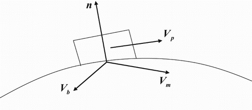
For unsteady inviscid flow, the boundary conditions are satisfied that the fluid normal velocity on the surface of a moving wing is equivalent to the surface moving velocity of the moving wall, (2) where is the fluid velocity on the body surface, is the moving velocity of the body surface and is the unit normal vector outward from the deformed body surface. The projection of in the tangent direction of the body surface is equal to that of in the tangent direction of the body surface, where is the fluid velocity at the centroid of the first layer. Thus, can be expressed as (3)

A sketch of the approximate boundary condition is shown in Figure 1. There are two advantages of using approximate boundary conditions; avoiding discontinuity of the grid due to interpolation at the interface of the multi-block grid, and avoiding the grid cross or negative volume caused by the large deformation of the wing.

Figure 1. The approximate boundary conditions.

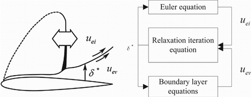
2.1.2. The Euler/boundary layer equation coupling method

Boundary layer equations are coupled with Euler equations to take fluid viscosity into account, in order to improve the calculation accuracy and efficiency. The integral equation of a compressible turbulent transition boundary layer is used. For three-dimensional models of engineering applications, a lifting surface can be divided into several strips. Each strip is calculated using integral boundary layer equations from the stagnation point along the top and bottom shunt lines. To avoid the occurrence of the Goldstein paradox, the ‘semi-inverse’ approach is adopted for iterative resolution. Figure 2 shows the principle diagram for the iterative resolution between the Euler equations and the boundary layer equations (Z. Zhang et al., 2004), according to the following steps:

1. Giving the initial boundary layer thickness distribution in advance.

2. Solving the shape function H, momentum thickness and outflow velocity in boundary layer equations.

3. Working out the boundary layer blow off or suction velocity along the outward normal vector.

4. Solving the Euler equations by iteration to get the external velocity near the boundary layer .

5. Updating the boundary layer thickness by the Cater or Edward relaxation iteration equation.

6. Judging whether the boundary layer thicknesses meet in both calculations, where is a very small positive real number. The calculation is finished if , otherwise is replaced with , and the calculations repeat from step (2) above, with the steps repeating until inequality is achieved.

Figure 2. The Euler/boundary layer coupling.

2.2. Solving structure problems

The structural dynamic equation is (4) where M is the structural mass, C is the damping, K is the stiffness matrix, f is the external exciting force vector (namely the aerodynamic force vector) and q is the structure displacement vector.

The structural deformation is approximated in the modal approach as (5) where the modal matrix is composed of eigenvectors and is the generalized displacement vector.

Substituting Equation (5) into Equation (4) gives (6)

The left and right sides of Equation (6) are multiplied by , (7) where is the generalized mass matrix, is the generalized damping matrix, is the generalized stiffness matrix and is the generalized force vector. and are diagonal matrices as follows: (8)

Using the modal method, the efficiency of the calculation can be improved. The modal approach only requires a small number of the lowest-frequency modes for flutter boundary prediction or dynamic loads analysis, and thus is more efficient than solving Equation (4) directly, involving the full dimension of the finite-element method structure. This method plays an important role in the calculation of the flutter and dynamic responses, although it is necessary to select the appropriate calculation modes.

2.3. The coupling method

A loosely-coupled method is used in this paper, which makes the engineering realization more convenient and efficient than using a close-coupled method. It only needs to call a CFD solver once at each time step, as a simplification of the close-coupled method which requires every time step to reach the state of convergence. Figure 3 presents the principle sketch of the loosely-coupled method. At each time step, the four phases are as follows:

1. Transferring data from the fluid part to the structural part and converting the surface pressure to the generalized aerodynamic forces imposed in structural motion equations.

2. Developing structural motion equations, and updating the generalized displacement vector and generalized velocity vector.

3. Transferring data from the structural part to fluid part, and the aerodynamic grid on the wing surface is deformed according to the structural deformation.

4. Calculating the flow field again with the updated boundary conditions and updating the variables of the flow field.

Figure 3. A ‘loosely coupled’ method.

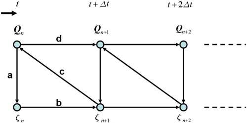
By repeating steps (1) to (4) above, the time history of the flow field and structure motion are obtained.

2.4. Transonic flutter analysis in the frequency domain

Traditional flutter methods in the frequency domain, such as the p-k method, v-g method and g method, are the methods most commonly used by engineers. However, a significant amount of work is required to convert the equations from the time domain to the frequency domain in the fluid–structure coupling system, such as fluid equations, structural motion equations and so on. The system-identification method is adopted for changing the time domain unsteady aerodynamic forces from the time domain to the frequency domain. Structural displacement and velocity could be considered as input while the aerodynamic coefficients could be regarded as output. The frequency-response characteristics of the system represent the generalized unsteady aerodynamic influence matrix, which can be used to solve flutter using the p-k or g method.

Because of the derivation based on linear theory, a quasilinear assumption should be made for the unsteady flow field. The steady flow field is nonlinear, which represents the existence of nonlinear factors such as shock waves, boundary layers and so on. There is another assumption that the structural response is a small disturbance, so the unsteady aerodynamic forces caused by the structure can be considered as small linear quantities relative to the steady aerodynamic forces.

2.4.1. Aerodynamic identification

Kreiselmaier and Laschka (2000) obtained the generalized aerodynamic forces (GAFs) by solving the linearized Euler equation. This method was used by Z. Zhang, Yang, and Chen (2012) to solve aeroelastic problems.

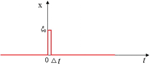
The aerodynamic identification method can also be used to calculate the real and imaginary parts of generalized aerodynamic coefficients under different structural modes and reduced frequencies. A time series can be chosen with a higher power spectral density in the relevant frequency bands, so the generalized aerodynamic coefficients of all frequencies can be solved by one time identification for each mode. The power spectral densities of white noise and the pulse time series are uniformly distributed across the whole frequency domain, which can be used as excitation signals. And the pulse signal is simple, so it is chosen as the excitation. Figure 4 shows a sketch of this, and the expressions are as follows: (9)

Figure 4. The pulse signal.

The frequency response of the pulse signal is (10)

The amplitude spectrum of the pulse signal is (11)

The amplitude spectrum of the pulse signal is shown in Figure 5. The fundamental frequency is . From Figure 5, it can be seen that the frequency information of f₀, 2f₀, … , nf₀ is lost. Therefore, should be set smaller to avoid the loss of vibration information, so that the fundamental frequency should be higher than the concerned elastic vibration frequency.

Figure 5. The amplitude spectrum of the pulse signal.

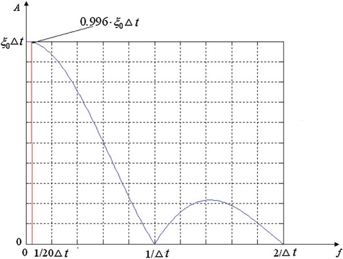
In the [0 (1/20)f₀] range, the amplitude of the frequency response is approximately a constant of . Taking the highest frequency of the flutter for example, the identification of the time step is set as 1/(20f_max) (20 time steps will be calculated in one period of the highest frequency). The amplitude of the frequency response is a constant of in the [0 ] range, so should be set as 1/(20f_max), which can cover the frequencies of the relevant structure modes.

If the given generalized displacement of the j-order mode is the pulse signal as shown in Equation (9), the aerodynamic coefficients y_1j(t), y_2j(t), … ,y_nj(t) of all modes are easy to solve, where represents the generalized aerodynamic coefficient of the i-order mode caused by the j-mode generalized displacement pulse input. Then the discrete Fourier transformation is used to handle the time series y: (12) where l represents the number of selected discrete points in the time series, b is the reference half chord length, is the fluid speed and k is the reduced frequency. The reduced frequency describes the flow characteristics changing with the time and represents the interaction of the motion with each point on the wing. The reduced frequency is defined as k = ωb/V, where ω is the circular frequency of the wing and V is flight speed. The frequency response function is the generalized unsteady aerodynamic coefficients (13)

The generalized displacement pulse responses of the n modes are calculated in turn and then the frequency response functions are solved by Equation (13), and finally the generalized unsteady aerodynamic coefficient is assembled into a matrix as follows: (14)

The generalized aerodynamic coefficient matrices H(k₁), H(k₂), … ,H(k_n) under the chosen reduced frequency series are obtained, which are used for flutter calculation in the frequency domain.

2.4.2. The flutter analysis method

The frequency domain generalized aerodynamic force matrix H(k) can be plugged into ZAERO for flutter analysis using the g method (ZONA Technology, 2011).

3. Model validation

Flutter wind-tunnel experiments using the AGARD445.6 wing were completed in a transonic dynamic tunnel (TDT) at the National Aeronautics and Space Administration (NASA) research center in Langley (Yates, 1987). Five different groups of models were designed, including four kinds of rigid models and one flexible model. The experiment of the AGARD445.6 flexible wing model has become a classical assessment for the transonic aeroelasticity calculation program.

3.1. Aerodynamic model

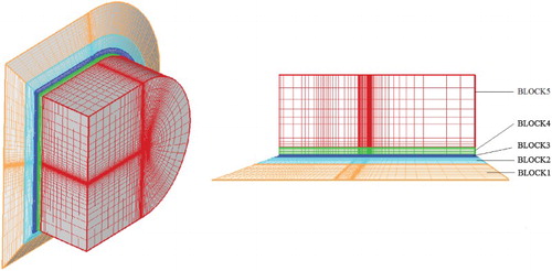
The computational domain is divided into five blocks of C-H grids (Figure 6). The body boundary conditions for the wing surfaces are set as walls, the symmetry plane of the airplane is set as the symmetric boundary condition, and finally the far-field surfaces from the airplane are set as the far-field boundaries.

Figure 6. The AGARD445.6 wing grids for CFD calculation.

3.2. Wing-structure model

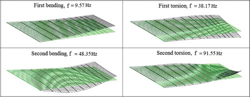
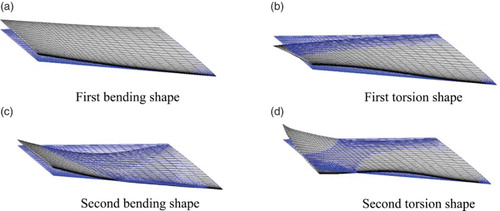
The structure model of the AGARD 445.6 wing is divided by 10 points in both the chordwise and spanwise directions (Figure 7). The first four modes are used for flutter analysis, with the mode frequencies and modal information given in Figure 8.

Figure 7. The structural finite-element model of the AGARD445.6 wing.

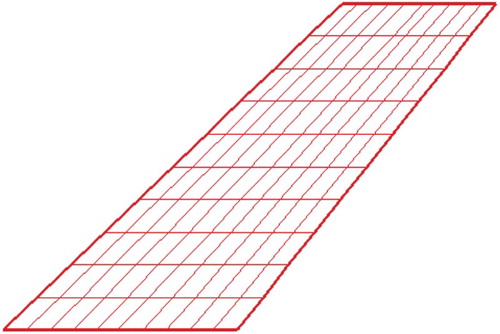
Figure 8. The first four mode frequencies and modal shapes of the AGARD445.6 wing.

4. Flutter analysis

4.1. Steady aerodynamic analysis

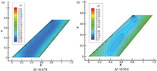
The transonic region is the primary concern when it comes to the flutter boundary, and four cases are be analyzed where M = 0.678, M = 0.901, M = 0.954, and M = 1.072, according to the experimental data. First, the Euler equations are marched to obtain a temporal convergent solution, then the Euler/boundary layer equations are used iteratively to obtain the final convergent state. The static pressure distributions for M = 0.678 and M = 0.954 at this stage are shown in Figure 9.

Figure 9. The steady pressure distributing cloud graphs of the AGARD445.6 wing.

4.2. CFD/CSD coupling calculation

4.2.1. Structure–fluid interpolation

All the structural grids are chosen as structural interpolating nodes and all the aerodynamic body surfaces are chosen as aerodynamic interpolating surfaces. The infinite plate spline (IPS) method (Rodden & Johnson, 1994) is used for the data transformation between fluid parts and structure parts. The structural modes are interpolated to the aerodynamic grids (Figure 10). Smooth and continuous interpolation can be used to accurately describe the structure modal shapes (Figure 8).

Figure 10. The modal shape interpolation graphs of the AGARD445.6 wing aerodynamic body surface grids.

4.2.2. Flutter analysis

Taking the example of M = 0.954, the responses of each mode are calculated with the chosen amplitude and the time step is 0.0002 s. Figure 11 shows the generalized aerodynamic response of the first two modes under the time step input, and Figure 12 shows the generalized unsteady aerodynamic forces of the first two modes changing with the reduced frequency. Finally, the v-g-f curves are shown in Figure 13. The generalized unsteady aerodynamic forces are used for the flutter analysis via the g method. The dimensionless flutter speed is , and the dimensionless frequency is . The first bending mode of the wing passes through the line g = 0 on the v-g graph, and the frequencies of the first bending and first torsion modes are increasingly close as the velocity increases, because the flutter mechanism is in the typical bending-torsion coupling mode (Figure 13).

Figure 11. The generalized aerodynamic responses of the step-input of the first two modes of the AGARD445.6 wing for M = 0.954.

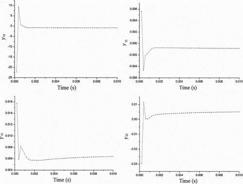
Figure 12. The generalized unsteady coefficients changing with the reduced frequency for M = 0.954.

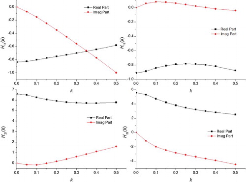
Figure 13. The v-g-f curves of the AGARD445.6 wing for M = 0.954.

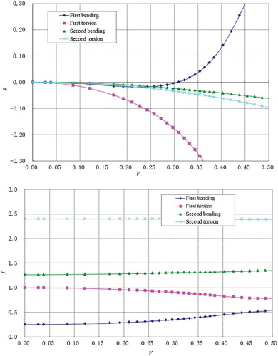
The generalized aerodynamic coefficient matrices, flutter velocities and flutter frequencies under the other Mach numbers are calculated in the same way: V_f = 0.434 and ω_f = 0.509 for M = 0.678; V_f = 0.354 and ω_f = 0.399 for M = 0.901; and, V_f = 0.426 and ω_f = 0.452 for M = 1.072. Their flutter mechanism is the bending-torsion coupling mode.

The CFD/CSD coupling method in the time domain is also adopted in this paper to analyze the flutter boundary of the AGARD445.6 wing. The analysis results for M = 0.954 are shown in Figures 14–16.

Figure 14. The generalized displacement response history for the time domain method when M =   0.954, V_f = 0.301 and g = −0.0031.

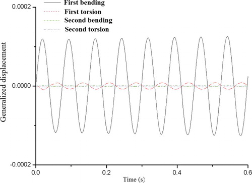
Figure 15. The generalized displacement response history for the time domain method when M =   0.954, V_f = 0.290 and g = 0.0025.

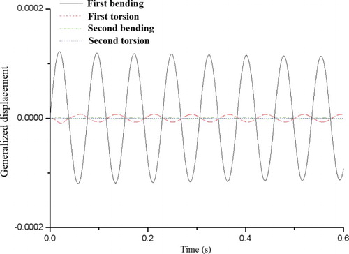
Figure 16. The generalized displacement response history for the time domain method when M  =  0.954, V_f = 0.295 and g = 0.00012.

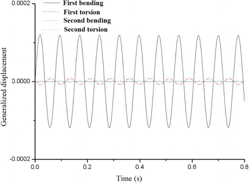
From Figures 14–16, it can be seen by observing the magnitude of generalized displacement of each mode that the flutter speed of the AGARD445.6 wing under Mach 0.954 is 0.295. The details of the generalized structural damping g are given in Li and Lu (2004). Figure 16 shows that the magnitude of generalized displacement of the first bending and torsion mode is larger than that of the other modes, which means that the flutter mechanism is the typical bending-torsion coupling mode. When flutter occurs at Mach 0.954, the generalized displacement response history of each mode obtained by the present method is shown in Figure 17, which shows that the results correlate well with the generalized displacement response calculated by the time domain method as shown in Figure 16.

Figure 17. The generalized displacement response history for the frequency domain method when M =   0.954 and when flutter occurs.

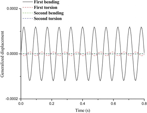
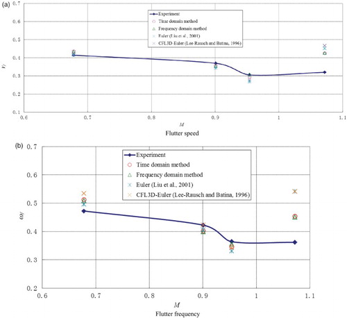
Figure 18 shows comparisons of the computed flutter boundary of the AGARD445.6 wing with the experimental data (Yates, 1987), and the results calculated by the CFL3D-Euler equations (Lee-Rausch & Batina, 1996) and Euler equations (Liu, Cai, Zhu, Tsai, & Wong, 2001). It can be seen that the simulation results are in accordance with the experimental results and the results obtained by other researchers for Mach numbers less than 1. The results are overestimated for Mach numbers greater than 1 because the flow field cannot be predicted accurately using the Euler/boundary layer equations coupling method presented in this paper, which needs further investigation. The simulation results of the CFD/CSD coupling method in the frequency and time domains are roughly the same, and the error is under 5%. The calculating efficiency of the frequency domain method presented in this paper is 3 to 4 times better than that of the time domain method.

Figure 18. The flutter boundary of the AGARD445.6 wing.

5. Conclusions

A method based on Euler equations is proposed for predicting transonic flutter boundary in this paper. Euler equations are considered for the fluid field and boundary layer equations are considered inside the boundary layers, taking viscosity into account. The prediction of the transonic flutter boundary is performed based on the traditional method in the frequency domain using generalized aerodynamic coefficiency matrices. The comparisons between the simulation and experimental results of the AGARD 445.6 wing show that the simulation results are in accordance with the experiment results for Mach numbers less than 1. The transonic dip of the flutter boundary of the AGARD445.6 wing is located at a Mach number of around 0.954, which is also the Mach number when the shock wave appears on the wing surface. The presented method is much more efficient than the time domain method. Since the simulation results are overestimated in the case of Mach numbers greater than 1, further study is ongoing to investigate the feasibility of using the Navier–Stokes algorithm to solve aeroelastic problems under this condition.

Disclosure statement

No potential conflict of interest was reported by the authors.

References

- Albano, E., & Rodden, W. P. (1969). A doublet-lattice method for calculating lift distributions on oscillating surfaces in subsonic flows. AIAA Journal, 7, 279–285. 10.2514/3.5086
- Fairuz, Z. M., Abdullah, M. Z., Yusoff, H., & Abdullah, M. K. (2013). Fluid structure interaction of unsteady aerodynamics of flapping wing at low reynolds number. Engineering Applications of Computational Fluid Mechanics, 7(1), 144–158. doi:10.1080/19942060.2013.11015460
- Farhangnia, M., Guruswamy, G. P., & Biringen, S. (1996, January). Transonic-buffet associated aeroelasticity of a supercritical wing. Paper presented at the meeting of AIAA 34th Aerospace Sciences Meeting and Exhibit, Reno, NV.
- Foerster, M., & Breitsamter C. (2013, June). Computational aeroelastic analysis in time and frequency domain using non-linear and linearized Euler/Navier-Stokes methods. Paper presented at the meeting of International Forum on Aeroelasticity & Structural Dynamics, Bristol, UK.
- Gao, C., Luo, S., Liu, F., & Schuster, D. M. (2005). Calculation of airfoil flutter by an Euler method with approximate boundary conditions. AIAA Journal, 43, 295–305. 10.2514/1.5752
- Gordnier, R. E., & Melville, R. B. (2001). Numerical simulation of limit-cycle oscillations of a cropped delta wing using the full Navier-Stokes equations. International Journal of Computational Fluid Dynamics, 14, 211–224. 10.1080/10618560108940725
- Iovnovich, M., & Raveh, D. E. (2012). Reynolds-averaged Navier-Stokes study of the shock-buffet instability mechanism. AIAA Journal, 50, 880–890. 10.2514/1.J051329
- Kreiselmaier, E., & Laschka, B. (2000). Small disturbance Euler equations: Efficient and accurate tool for unsteady load prediction. Journal of Aircraft, 37, 770–778. 10.2514/2.2699
- Lee-Rausch, E., & Batina, J. T. (1996). Wing flutter computations using an aerodynamic model based on the Navier-Stokes equations. Journal of Aircraft, 33, 1139–1147. 10.2514/3.47068
- Li, D., & Lu, Q. H. (2004). Analysis of experiments in engineering vibration. Beijng: Tsinghua University Press.
- Liu, F., Cai, J., Zhu, Y., Tsai, H. M., & Wong, A. S. F. (2001). Calculation of wing flutter by a coupled fluid-structure method. Journal of Aircraft, 38, 334–342. doi:10.2514/2.2766
- Obayashi, S., & Guruswamy, G. P. (1995). Convergence acceleration of a Navier-Stokes solver for efficient static aeroelastic computations. AIAA Journal, 33, 1134–1141. doi:10.2514/3.12533
- Rodden, W. P., & Johnson, E. H. (1994). MSC/NASTRAN aeroelastic analysis: User's guide (Version 68). Los Angeles, CA: MacNeal-Schwendler Corporation.
- Sadeghi, M., Yang, S., Liu, F., & Tsai, H. M. (2003, January). Parallel computation of wing flutter with a coupled Navier-Stokes/CSD method. Paper presented at the meeting of 41st Aerospace Sciences Meeting and Exhibit, Reno, NV.
- Wang, G., Mian, H. H., Shan, X., & Lee, J. (2015). Static aeroelastic predictions for complex aircraft configurations with CFD/CSD coupling methodology. AIAA Journal, 7, 279–285. doi:10.2514/6.2015-0253
- Yates E. C. (1987). AGARD Standard Aeroelastic Configurations for Dynamic Response candidate configuration I-Wing 445.6. NASA TM-100492.
- Zeng, X., Xu, M., An, X., & Chen, S. (2008). Wing flutter analysis using CFD/CSD algorithm. Journal of Northwestern Polytechnical University, 26 (1), 79–82. 10.3969/j.issn.1000-2758.2008.01.016
- Zhang, W. (2006). Efficient analysis for aeroelasticity based on computational fluid dynamics (Doctoral dissertation). Retrieved from China Doctoral Dissertations Full-text Database. doi:10.7666/d.y1189904
- Zhang, W., Jiang, Y., & Ye, Z. (2007). Two better loosely coupled solution algorithms of CFD based aeroelastic simulation. Engineering Applications of Computational Fluid Mechanics, 1, 253–262. doi:10.1080/19942060.2007.11015197
- Zhang, Z., Liu, F., & Schuster, D. M. (2004, August). Calculations of unsteady flow and flutter by an euler and integral boundary-layer method on Cartesian grids. Paper presented at the meeting of 22nd Applied Aerodynamics Conference and Exhibit, Providence, Rhode Island.
- Zhang, Z., Yang, S., & Chen, P. C. (2012). Linearized Euler solver for rapid frequency-domain aeroelastic analysis. Journal of Aircraft, 49, 922–932. doi:10.2514/6.2011-3364
- ZONA Technology. (2011). ZAERO theoretical manual. Scottsdale, AZ: ZONA Technology.