Rotor wake and flow analysis using a coupled Eulerian–Lagrangian method

ABSTRACT

A coupled Eulerian–Lagrangian methodology was developed in this paper in order to provide an efficient and accurate tool for rotor wake and flow prediction. A Eulerian-based Reynolds-averaged Navier–Stokes (RANS) solver was employed to simulate the grid-covered near-body zone, and a grid-free Lagrangian-based viscous wake method (VWM) was implemented to model the complicated rotor-wake dynamics in the off-body wake zone. A carefully designed coupling strategy was developed to pass the flow variables between two solvers. A sample case of a forward flying rotor was performed first in order to show the capabilities of the VWM for wake simulations. Next, the coupled method was applied to rotors in several representative flight conditions. Excellent agreement regarding wake geometry, chordwise pressure distribution and sectional normal force with available experimental data demonstrated the validity of the method. In addition, a comparison with the full computational fluid dynamics (CFD) method is presented to illustrate the efficiency and accuracy of the proposed coupled method.

KEYWORDS:

• Rotor wake
• coupled Eulerian–Lagrangian method
• Navier–Stokes equations
• viscous wake model
• CFD

Nomenclature

	=	Sound speed (m/s)
	=	Rotor blade chord (m)
	=	Overlap factor
	=	Rotor thrust coefficient,
	=	Pressure coefficient
	=	Normal force coefficient
	=	Minimum vortex size, non-dimensionalized by R
	=	Rotor tip Mach number
	=	Rotor radius
	=	Rotor-wake cut-off distance, non-dimensionalized by R
	=	Radial position along the blade span
	=	Rotor thrust
	=	Velocity field
	=	Rotor tip velocity
x	=	(x, y, z) Cartesian coordinates, non-dimensionalized by R
	=	Collective pitch
	=	Rotor advance ratio,
	=	Air density
	=	Blade azimuthal angle
	=	Rotor angular velocity (rad/s)
	=	Magnitude of vorticity, non-dimensionalized by
	=	Free stream

1. Introduction

The flow around helicopter rotor blades is highly complex, characterized by flow phenomena such as shock waves, dynamical stalls and separated flow. Additionally, the highly energetic concentrated tip vortex generated and rolled up in the blade tip region constantly remains within the vicinity of the operating blades. The close interaction between the wake and the blade may lead to impulsive airloads and increase the rotor’s vibration and noise levels (Bhagwat, Ormiston, Saberi, & Xin, 2012). Given the complexity stated above, rotor-wake dynamics and performance predictions remain the most challenging tasks for rotor aerodynamics modeling.

Computational fluid dynamics (CFD) technology was first applied to rotorcraft research in the 1970s, and significant improvements have been achieved over the past several decades as a result (Strawn, Caradonna, & Duque, 2006) The modern Eulerian-based CFD method models the whole rotor system using a multi-block strategy (e.g. overset grid, deforming mesh) and attempts to capture the wake structure entirely from first principles by solving the Navier–Stokes equations (Ahmad & Duque, 1996; Kang & Kwon, 2002; Zhao, Xu, & Zhao, 2005). However, the numerical dissipation and interpolation errors inherent to the difference schemes employed the causes the rotor wake to be modelled with less intensity than occurs in physical reality. Certain specific algorithms, such as grid refinement and high-order accuracy schemes, have been employed in recent investigations – but the capability to capture the rotor wake at a sufficient resolution is yet to be demonstrated (Dimanlig, Jayaraman, Lim, & Wissink, 2012; Duraisamy & Bader, 2007; Harris, Sheta, & Habchi, 2010; Liu, Yang, Wu, Tian, & Du, 2014). Furthermore, vast amounts of computation time and resources hinder their applications in the helicopter industry. An alternative methodology is to incorporate the external wake model into the CFD solution. This combines the merits of the CFD and vortex solutions and is computationally efficient. Some notable investigations into coupling methods have been reported in the literature, and their results are in good agreement with the measured data, obtained while dramatically reducing the required computation time (Bhagwat, Moulton, & Caradonna, 2007; Shi, Zhao, Fan, & Xu, 2011; Sitaraman & Bader, 2006; Wie, Im, Kwon, & Lee, 2010; Yang, Sankar, & Smith, 2002). However, limitations still exist regarding the singularity-based vortex module used in these coupling methodologies (Komerath, Smith, & Tung, 2011). Because of the assumption of inviscid flow, the wake solutions have to rely on empirical formulations that are used to account for the roll-up rule, initial vortex core size, and vortex decay factor.

To overcome the shortcomings of the existing coupling methods, a novel method which couples CFD with the viscous wake method (VWM) is proposed in this paper for rotor-wake and flow prediction. In the coupled CFD/VWM method, a compressible Reynolds-averaged Navier–Stokes (RANS) solver is used to simulate a small region covering the blade and predict the blade airloads; the VWM, which addresses solutions through the Lagrangian formulation of incompressible Navier–Stokes equations (Brown & Line, 2005; He & Zhao, 2009; Tan & Wang, 2013; Wei, Shi, Xu, & Zhao, 2012), is employed to model the complicated rotor-wake dynamics without artificial dissipation. The details of the coupling algorithm are described in this paper. To assess the method, several numerical samples for rotors in hover and forward flight conditions were carried out and the results are compared with measured data.

2. Coupling methodology

Figure 1 shows a schematic diagram of the coupled Eulerian–Lagrangian method. In the grid-covered near-body zone, the Eulerian-based CFD method is employed to predict the blade airloads and complex aerodynamic phenomena, and to pass the generated vorticity to the VWM, while a Lagrangian-based VWM is used to model the rotor-wake dynamics in the off-body wake zone and couple back the wake-induced velocity to the CFD domain. The details of this method are described below.

Figure 1. Schematic diagram of the presented coupling method.

2.1. CFD solver

A full CFD method incorporating a moving overset grid system has been developed by our research group. The validation of the code is demonstrated through a wide range of applications, i.e. single rotor, rotor/fuselage interaction, and rotor noise (Fan, Xu, & Shi, 2014; Shi et al., 2011; Wang, Zhao, Xu, & Ye, 2013; Ye, Zhao, & Xu, 2009; Zhao et al., 2005). In this CFD solver, the three-dimensional, unsteady compressible RANS equations were employed as the governing equations, which can be written as: (1) where In the above equations, is the vector of conserved variables, and are the convective (inviscid) and viscous flux vectors, respectively, is the absolute velocity, is the blade moving velocity including blade rotation, flapping and pitching motions, and are the density, pressure and energy, respectively, is the cell volume, is the face area, is the normal vector of the grid face, encapsulates the components of the viscous stress tensor, and encapsulates the terms describing the work of viscous stresses.

The inviscid terms were computed using a second-order upwind Roe scheme (Roe, 1981) and the viscous terms were computed using second-order central differencing. For the time integration, a dual time stepping method was applied with the lower-upper symmetric Gauss-Seidel scheme (Luo & Baum, 1999) to simulate the unsteady flow phenomenon at every pseudo time step. The Spalart–Allmaras turbulence model (Spalart & Allmaras, 1992) was employed for the RANS closure.

2.2. Viscous wake method

A VWM was employed to model rotor-wake dynamics in this study. It comprises the rotor-wake dynamics model and rotor aerodynamics model. The mathematical and numerical formulation of VWM has been extensively documented (He & Zhao, 2009; Tan & Wang, 2013; Wei et al., 2012). Here, only the essential details are given.

2.2.1. Rotor-wake dynamics model

The airflow around the rotor is incompressible except for a small region around the blade tip. Therefore, rotor-wake dynamics can be described by vorticity kinematic and dynamic equations (a vorticity-velocity formulation of the incompressible Navier–Stokes equation): (2) where is the vorticity field associated with the velocity field u, is the kinematic viscosity, and is the position of the vortex. In the VWM, the vorticity is discretized into the regular distributed vortex particles in which the vorticity is concentrated (Chorin, 1973). The rotor-wake field is represented by a set of N Lagrangian vector-valued particles as (3) where is the position of the particle, is the vector-valued total vorticity inside particle p, is the smoothing parameter and is the smooth cut-off function.

Combining Equations (2) and (3), the governing equation can be rewritten as (4) (5) and , where is the free stream velocity and is the local induced velocity.

The first term on the right-hand side of Equation (5) is the stretching-effect term. In the current simulation, the velocity gradient can be obtained by analytically differentiating the velocity field. Using a transposed formulation, the stretching-effect term can be written as (6)

The second term is the viscous diffusion term, which can be solved using the particle strength exchange technique (Eldredge, Leonard, & Colonius, 2002). In actuality, only a subset of all the particles needs to be considered when integrating over the volume of particle p; the viscous diffusion term can be written as (7)

The direct evaluation of particle convection velocity and velocity gradient requires O(N²) operations (where N denotes the number of particles), thus rendering the method unacceptable for large N simulations. In this study, the fast multipole method (Cheng, Greengard, & Rokhlin, 1999) has been implemented to accelerate the calculation process.

2.2.2. Rotor aerodynamics model

The blade surface is treated as the only vorticity source that generates vortex particles in the rotor wake. The circulation of the blade-bound vortex and new vortex particles can be calculated by using a lifting line (surface) model or non-linear CFD method.

The circulation of the bound vortex varies both azimuthally and spanwise, thereby generating shed and trailed vortices in the rotor wake. The shed and trailed vorticities are calculated from the time and radial derivatives of the bound vortex, respectively. Therefore, at each time step, the vorticity of the new vortex can be written as (8)

where is the circulation of the blade bound vortex, is the sectional relative flow-field velocity (including the free stream velocity and the blade motion velocity), and ω is the total vorticity of both the shed and trailed vortices from the aerodynamic model. Then, the vorticity strength in the previous equations is calculated as (9)

2.3. Coupling algorithm

A carefully designed coupling strategy is required to pass the vorticity of the CFD to the VWM and couple the induced velocity of the VWM back to the CFD solution. The details of the treatment of the boundary conditions are as follows.

2.3.1. CFD to VWM solution

In the present coupling method, the ‘integrated vorticity approach’ (Shi et al., 2011) is adopted to pass the vorticity from the CFD domain to the VWM solution. In this approach, the circulation strengths are computed using the sectional lift coefficient integrated from the pressure distributions on the blade surface; the bound vortex strength is then given using the Kutta–Joukowski theorem, (10) where is the sectional lift coefficient and is the local flow velocity.

As the tip vortex strength is obtained, the newly generated vortex for VWM can be calculated using Equations (8) and (9).

2.3.2. VWM to CFD solution

In the coupling method, the flow variables in the CFD domain are calculated by including the influence of the induced velocity of the rotor wake from the VWM. The ‘outer boundary correction’ approach (Shi et al., 2011) is used to pass the velocity from the VWM to the CFD solution. In this approach, the induced velocity associated with the VWM is only imposed on the outer boundary of the blade grid to satisfy the mass conservation, and the CFD domain is computed under the specified outer boundary condition and the necessary inner boundary conditions. Compared to the field-velocity approach (Sitaraman & Bader, 2006), in which it is necessary to calculate the induced velocities at all grid points, the simplicity and efficiency of this method are great advantages.

The density, energy and pressure, in addition to the wake-induced velocity, need to be specified at the outer boundary for a compressible CFD solution. The variables can be obtained from the following equations: (11) where (u_a, v_a, w_a), (u_g, v_g, w_g) and (u_i, v_i, w_i) are the free-stream velocities, blade moving velocities and wake-induced velocities, respectively, is the ratio of specific heat, is the local Mach number, and is the free stream.

As mentioned previously, the induced velocities need to be recalculated every time step. However, the near wake sheet – which is assumed to roll up into a tip vortex at 30° of the azimuthal angle – is computed as part of the CFD solution. To avoid the double counting of the near wake sheet, the first 30° of the wake geometry of the VWM are excluded from the induced-velocity calculations.

2.3.3. Flow chart of the coupling method

Figure 2 shows the flow chart of the coupling method. The solution is carried out as follows:

1. Initialize and conduct the CFD and VWM solutions;

2. Calculate the spanwise sectional circulation around the blade from the CFD solution;

3. Generate the source term and solve the rotor wake using the VWM;

4. Calculate the induced velocity associated with the vortex particles and feed it back to the CFD domain.

Figure 2. Flow chart of the coupled CFD/VWM method.

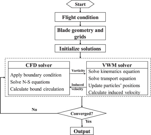
Steps 2 to 4 are repeated until convergence occurs. The time step in the VWM is commonly set as an integral multiple of the time step in the CFD solution for the sake of efficiency. In this paper, time steps of 0.25° and 1° are used for the CFD and VWM solutions, respectively. The sectional circulation and induced velocity were calculated every four stations, and the values were frozen until the new calculation could be updated.

3. Results and discussion

To validate the developed method, several test cases were performed and compared with available experimental data for different helicopter rotor configurations. Section 3.1 illustrates the capability of the VWM for rotor-wake simulations. Detailed investigations into the coupling method are reported in the following sections.

3.1. Rotor-wake modeling

In the VWM, the key parameters that affect the computational accuracy include the overlap factor , minimum vortex size , and wake cut-off distance . The number of vortex elements N_vp is determined by these parameters.

An isolated four-bladed rotor (Elliott, Althoff, & Sailey, 1988) in forward flight where , , and was performed. The rotor has four blades with radii of R = 0.861 m and a linear negative twist of −8°. The computational parameters were set as , , and , and more than 31,000 vortex elements were identified after computation.

Figure 3 shows the predicted rotor-wake structure and the time-averaged induced downwash variation. In forward flight, the rotor wake is asymmetrical around the lateral axis. The inclined wake structure results in upwash at the front of the rotor disk and a strong downwash at the rear (the blade azimuthal angle ), while slightly affecting the lateral downwash distribution (). In the figures, the numerical results from the potential-flow-based free wake method (Bagai & Leishman, 1995) are also shown. Given the potential-flow assumption, the free wake method has to rely on an empirical formulation to obtain the rotor-wake solution, thus capturing the distribution but not the magnitude of the inflow variation. In contrast, the current method predicts the correlation of inflow variation using the measured data (Elliott et al., 1988), particularly near the blade tip region. The inclusion of the viscous effect on the vortex convection contributes to the acquisition of a more accurate wake structure. Figure 4 gives a non-dimensional time-varied induced downwash of two radial positions at . The instantaneous velocity greatly influences airload prediction and is difficult to predict accurately. As shown in the figure, the periodicity due to blade rotation is captured, and the amplitude and phase angle of the induced downwash are in agreement with the measured data. These features are crucial for the accurate prediction of airload on the blade surface.

Figure 3. Predicted rotor-wake structure and wake-induced downwash for a rotor in forward flight: (a) rotor-wake geometry and (b) radial distribution of the wake-induced downwash.

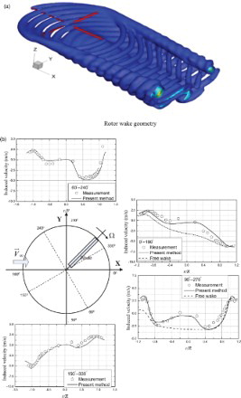
Figure 4. Time-varied wake-induced downwash at 0° azimuthal angle for (a) r = 0.74R and (b) r = 0.86R.

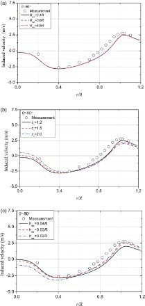
For the coupling method, the induced velocity is the most important factor that contributes to the accuracy of the results. Therefore, a sensibility study of computational parameters on the wake solution was carried out. Figure 5(a) shows the effect of the wake cut-off distance . It denotes the far-wake distance from the hub center and determines the length or revolutions of the rotor wake. As shown, all results are nearly the same when the value varies from 2.4R to 4.8R. When , approximately 7 revolutions of rotor wake can be captured. This is more than the minimum value (about 4–6 revolutions) required for induced-velocity prediction, thus the wake resolution is sufficient for the coupling method. Generally, the value of ranges from 3R to 4R for the forward flight case, and is used in hover flight. Figure 5(b) shows the effect of the overlap factor , which exhibits an effect on the wake contraction (the radial displacement of tip vortex). As shown, a small overlap factor provides more accurate results. With the value increased, the downwash velocity is smoother in velocity mutation regions (blade tip vortex location), resulting in a poor fit with experimental data. However, if the value is too small then numerical instability results; thus, a minimum value of 1.0 is required in the solution to ensure convergence. In computations, the value of usually ranges from 1.2 to 1.4. Figure 5(c) shows the effect of the minimum vortex size on the rotor downwash prediction. It governs the number of vortex particles. In this numerical case, 11,525 vortex particles are generated at the end of the calculation when while the number is 24,707 when . Although a more accurate result is shown in the figure with the smaller , the computation time also increases dramatically. Taking both accuracy and efficiency into account, the value of is usually set at 0.03R.

Figure 5. Effects of the computational parameters on the rotor-induced velocity for (a) the wake cut-off distance, (b) the overlap factor, and (c) the minimum vortex size.

3.2. The hover case

A two-bladed Caradonna–Tung (Caradonna & Tung, 1981) rotor in the hover case is studied in this section. The rotor operates at . For comparison, the same case was conducted using the full CFD method developed by our research group.

In the hover case, the flow field can be seen as steady in the rotation coordinate system, in which case only one blade is needed to model with the periodic boundary condition as it is introduced. As shown in Figure 6, a half-cylinder background mesh and a body-fitted blade grid were used. The background mesh contains 7.2 million grid points with the dimensions 141×270×190. To improve the capture of the rotor wake, the grids were clustered at the regions around and below the rotor, and the minor grid size was about 0.05c. A C-O-type body-fitted grid containing 398,412 grid points (with the dimensions 189×31×68) was used to model the blade, and the outer boundary extended approximately 1.5c from the blade surface.

Figure 6. Overset grid system for the hover case: (a) C-O-type blade grid and (b) half-cylinder background mesh.

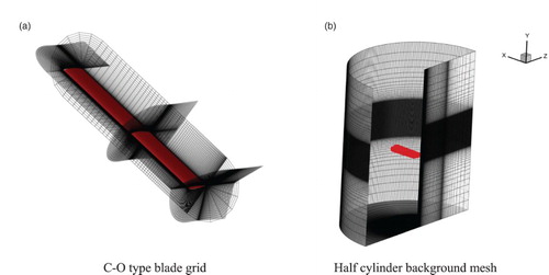
Figure 7(a) shows the predicted rotor-wake structure with a non-dimensional vorticity magnitude of . In the hover case, the rotor tip vortex quickly contracts after releasing from the blade and diffuses gradually during convection. The full CFD method captured approximately 4 revolutions of the rotor wake. Figure 7(b) shows the vorticity iso-surface on a vertical slice across the rotor center. The highly concentrated tip vortex was captured during the first revolution. As the tip vortex convected downstream, significant numerical diffusion occurred in the vortex core region, resulting in vortex diffusion and distortion. For the purpose of illustration, the grid distribution has been superimposed on the figure. Although the grids were refined in the wake convection region, the cell size was still too large for rotor tip vortex simulation. To preserve the wake structure and improve the prediction of hover performance, a high-density grid of a size of less than 0.01c (more than 10 grid points distributed within a vortex core) should be used. Unfortunately, this results in a massive increase in computational resources and time.

Figure 7. Predicted rotor-wake structure from the full CFD method (Caradonna–Tung rotor): (a) rotor-wake geometry () and (b) vorticity contour slice crossing the rotor center.

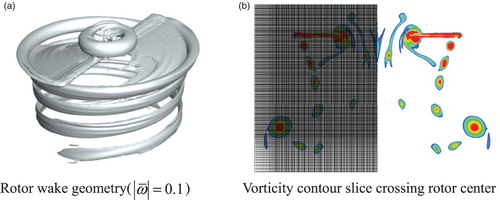
Figure 8. Computational domain of the coupling method for the hover case.

Next, we investigated the rotor-wake prediction of the coupling method. Figure 8 illustrates the computational domain used for this sample case. The blade grid was the same as the one used in the CFD method. The wake solution domain extends 2R below the rotor plane. The computational parameters were set as , , and . About 32,648 vortex elements were generated. Figure 9 shows the predicted rotor-wake structure with a non-dimensional vorticity magnitude of . As shown, several revolutions of rotor tip vortex were captured, and the vorticity was concentrated during convection with very little physical diffusion. In addition, mutual interaction and the distortion of vortex filaments, which occurred at one radius below the rotor plane, are also illustrated in this figure. Figure 10 shows the radial and vertical displacements of the tip vortex varying with wake age. The predicted results correlate well with the measured data (Caradonna & Tung, 1981). Overall, the results above indicate that the coupling method is capable of rotor-wake prediction.

Figure 9. Predicted rotor-wake structure from the coupling method (Caradonna–Tung rotor in the hover case): (a) rotor-wake geometry () and (b) vorticity contour slice crossing the rotor center.

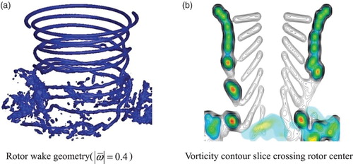
Figure 10. Predicted radial and axial displacements of the rotor tip vortex.

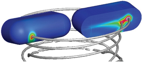
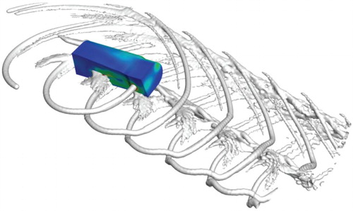
Next, we checked the consistency of the two solutions. Figure 11 shows a close-up of the tip vortex at , illustrating the flow-field information interchange between the two computational domains. The boundary condition approach, upon which the wake-induced velocity is imposed on the outer surface of the blade grid, was used to account for the wake effect feedback to the CFD domain. As shown, the tip vortex trailing from the proceeding blade passed through the CFD domain. The vorticity distribution at the outer boundary induced by the tip vortex is clearly apparent, which indicates the feasibility of the coupling stratagem used in the present method.

Figure 11. Close-up of the rotor tip vortex passing to the CFD domain.

Finally, the blade airloads were investigated. Figure 12 shows the predicted chordwise pressure distribution at two radial stations. The distributed pressure from the full CFD method and the coupling method agree with the experimental data (Caradonna & Tung, 1981), with the only minor discrepancy occurring in the leading edge region. The sectional lift coefficient distribution along the span is presented in Figure 13. As shown, the lift predicted by the coupling method was overestimated at the blade tip and underestimated in the inboard region. The integrated vorticity approach used for passing the CFD vorticity to the VWM may account for this error, which induces a smaller velocity at the blade tip than would occur in reality, and a larger value in the inboard region. In future studies, a distributed vorticity approach will be included in the solution to improve prediction accuracy.

Figure 12. Chordwise pressure coefficient distribution on the blade surface (Caradonna–Tung rotor in the hover case) for: (a) r/R = 0.68, (b) r/R = 0.80, (c) r/R = 0.89, and (d) r/R = 0.96.

Figure 13. Sectional lift coefficient distribution along the blade span.

Table 1 summarizes the computation time for the two methods. All sample calculations were performed on a workstation (Core2 E 7200 2.6G). In a steady CFD solution, only one blade grid and partial background grid are used. As shown, a typical hover solution requires about 28 hours for the full CFD method and 10 hours for the coupling method. These results indicate that the coupling method dramatically reduces the required computation time.

Table 1. Comparison of computation times between the coupling method and the full CFD method.

	Full CFD method (steady solution)	CFD/VWM
Blade grid	398,412	398,412×2
Background grid/particle number	7,233,300	32,648
Total time (hours)	28	10

3.3. Low-speed flight case

In this section a low-speed case of the Helishape 7A rotor (Biava, Bindolino, & Vigevano, 2003) was used to demonstrate the reliability of the coupling method in the forward flight case. The four-bladed 7A rotor is articulated with a radius of R = 2.1 m, aspect ratio of 15, and solidity σ = 0.0849. The rotor operates at Ma_tip = 0.617 and μ = 0.167. In this low-speed descending flight, the rotor operates in a representative blade-vortex interaction (BVI) condition. The control inputs and blade flap motions were obtained from experimental data.

Figure 14 shows the computational domain of the coupling method for the forward flight case. The C-O-type blade grid has the dimensions 189×31×71. The computational parameters were set as R_cut = 3R, = 1.3 and h_res = 0.03R. About 21,586 vortex elements were generated. Figure 15 shows the rotor-wake structure plotted in terms of the vorticity iso-surface from the coupling method. The non-dimensional vorticity magnitude in Figure 15(a) was set as . 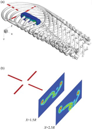Formation and rollup of the rotor tip vortex on the advancing and retreating sides were observed. Constrained by the size of the computational domain, approximately 5 revolutions of rotor tip vortex were captured, but that is sufficient for rotor performance predictions. Figure 15(b) shows the vorticity contour slices at two locations behind the rotor (x = 1.5R and 2.5R). As shown, the vortexes were confined within small regions, which means that the rotor wake was well preserved while traveling downstream.

Figure 14. Computational domain for the coupling method in forward flight.

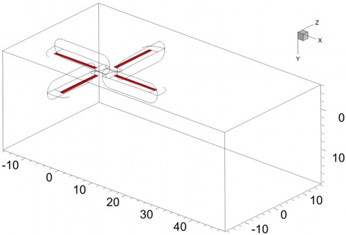
Figure 15. Predicted rotor-wake structure via the coupling method (7A rotor): (a) rotor-wake geometry and (b) vorticity contour slices.

In forward flight, the unsteady CFD solver must be employed to simulate the time-varied rotor flow-field. The overset grid system was comprised of a large-scale background mesh and four body-fitted grids for each blade (Figure 16). The background mesh had the dimensions 315×134×207. Figure 17 shows the wake solution results from the full CFD method. To display 4 to 5 revolutions of the rotor wake, a small vorticity magnitude of , which is one ninth of that used in the coupling method, is used in Figure 17(a). From the vorticity contour slices (Figure 17(b) and (c)), significant numerical diffusion is observed in the wake-developing zone, which caused the rotor tip vortex to diffuse rapidly as the vortex age grew. In addition, another type numerical error existing in the full CFD method was also observed in the simulation results. Affected by local induced velocity, the trailed rotor tip vortex moved downstream along the spiral trajectory in forward flight. When the tip vortex turned back, it entered the boundary regions of multi-blocks, where non-continuous interpolation is used for flow-field information transmission. The numerical errors arising from the interpolations caused the vortex to diffuse significantly. Therefore, the rotor-wake geometry shown in Figure 17(a) is incomplete. To further illustrate this phenomenon, the vorticity contour slice crossing the rotor center from two sample calculations are compared in Figure 18. As can be seen, it is evident that the vortex around the rotor has not been captured, which could have a significant impact on blade airload prediction.

Figure 16. Overset grid system used for the forward flight case.

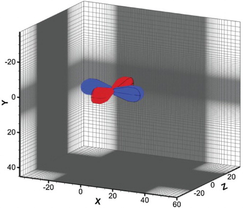
Figure 17. Rotor-wake structure predicted by the full CFD method (7A rotor): (a) rotor-wake geometry, (b) slice1, x = 1.5R, and (c) slice2, x = 2.5R.

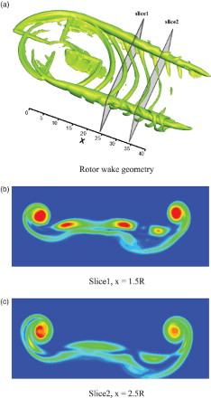
Figure 18. Vorticity contour on a vertical slice crossing the rotor center (7A rotor) for (a) the full CFD method and (b) the coupling method.

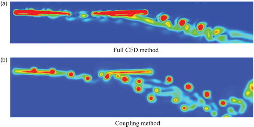
Figure 19 shows the predicted chordwise pressure distribution on the blade surface at the radial position 0.82R. As can be seen, the calculated pressures from the coupling method are in close agreement with the experimental data at three azimuthal angles, except at 90°, where the pressure is overestimated (Biava et al., 2003). This discrepancy could arise from the integrated vorticity source approach, which induces the smaller velocity at the blade tip region. The results from the overset method are also plotted in the figure. Although the rotor tip vortex was not well preserved in this solution, the calculated pressures correlate well with the measurements. The reason for this could be that the blade airload is most affected by the induced velocity arising from the tip vortex of the proceeding blade, which is simulated in the calculations shown in Figures 15 and 17.

Figure 19. Chordwise pressure distribution on the blade surface at 0.82R (7A rotor) for: (a) , (b) , (c) , and (d)

Figure 20. Time history of sectional normal force coefficient for (a) r/R = 0.82 and (b) r/R = 0.92.

Figure 21. Sectional normal force coefficient (3/rev and higher) for (a) r/R = 0.5, (b) r/R = 0.70, c) r/R = 0.82, and (d) r/R = 0.92.

The comparisons between the predicted time-history of sectional normal force with the experimental data (Biava et al., 2003) at two radial positions are shown in Figure 20. Because of the well-preserved tip vortex in the coupling method, the multiple BVI events – which occurred at the outerboard of the blade at 90° and 270° – resulted in oscillations of sectional lift at these locations. By contrast, only weak orthogonal BVI events existed on the blade due to numerical diffusion, and the predicted time-history of sectional lift varies gradually.

Figure 21 shows the 3/rev and higher harmonics of sectional normal force at four radial stations. These components are crucial for structure loading prediction and dynamics analysis. By comparing Figures 20 and 21, it is clear that the BVI-inducing oscillations of higher harmonic normal force are more pronounced, especially at the inboard blade. The discrepancy between Figures 20 and 21 has two potential causes. One is the inaccurate control inputs; in this solution, the trim procedure is not employed to obtain the collective and cycle pitches, andthus the values are taken from the experiment. The difference between the control inputs in the simulation and the experiment could cause a discrepancy. The other potential cause is the effect of blade elastic deformation. A rigid rotor model – which we consider to be only the first-order component of the flap and pitch motion – was used in the present coupling method, whereas the experimental rotor is elastic and the rotor undergoes flap and torsional deformation during rotation. Elastic deformations cause fluctuations in the sectional attack-angle of the blade, thereby changing the blade airloads. The larger discrepancy occurs at the outboard blade (see Figure 21(b) and (c)), where the elastic deformation is more significant than in the inboard region. In addition, the higher harmonics of normal force result in a high-order elastic deformation, which results in a larger discrepancy than the whole normal force in Figure 20. Overall, the BVI events are captured well by the coupling method, and its results are better than those of the full CFD method.

Table 2 presents the computation time of the full CFD and coupling methods; it can be seen that while the full CFD method requires 85 hours, only 12 hours are needed for the coupling method. In the forward flight case, the unsteady solver should be employed to model the rotor flow-field, thereby dramatically increasing the computation time of the full CFD method. However, the time of the coupling method changes little, due to the lower number of vortex particles used in the calculation.

Table 2. Comparison of computation time between the coupling method and the full CFD method for the forward flight case.

	Full CFD method (unsteady solution)	CFD/VWM
Blade grid	415989×4	415989×4
Background grid/particle number	8,737,470	21,586
Total time (hours)	85h	12h

3.4. High-speed flight case

Finally, a sample case for the full-scale UH-60 rotor (Kufeld & Bousman, 2005) in high-speed forward flight was performed. The fully articulated four-bladed rotor has a radius of 8.178 m and a solidity of 0.0832. The rotor operates at , , and and the control inputs were obtained from experimental data. The computational parameters were set as R_cut = 3R, = 1.3, h_res = 0.03R and N_vp = 14589. The C-O-type blade grid has the dimensions 191×46×98.

The rotor-wake structure, as well as the vorticity iso-surface at the outer boundary of the CFD domain, is plotted in Figure 22. For purposes of illustration, only one blade is shown. In the case of high-speed flight, the tip vortex moves downstream rapidly when released from the blade, thus having less effect on blade airloads and performance compared to the hover and low-speed flight cases.

Figure 22. Predicted rotor-wake structure using the coupling method (UH-60A rotor).

Figures 23 and 24 show the chordwise pressure distributions on the blade surface at four azimuthal angles and two radial stations. At the advancing side, the blade involves transonic flow and strong shock waves occur at the outboard blade where the maximum blade tip Mach number reaches . The coupling method captures the transonic phenomenon and the predicted results correlate well with the experimental data (Kufeld & Bousman, 2005). Figure 25 shows the sectional normal force at four representative radial stations. The apparent difference between the simulated and experimental results are shown at r/R = 0.865 and r/R = 0.965. Elastic deformation mainly contributes to the discrepancy in high-speed flight where the rotor blade undergoes more significant torsional deformation than in the low-speed case. Overall, the simulated results correlate well with the experimental data. These encouraging results have provided us with the confidence to develop an efficient tool for helicopter industry applications.

Figure 23. Chordwise pressure coefficient distribution at r/R = 0.775 (UH-60A rotor) for (a) , (b) , (c) , and (d) .

Figure 24. Chordwise pressure coefficient distribution at r/R = 0.865 (UH-60A rotor) for (a) , (b) , (c) , and (d) .

Figure 25. Section normal force coefficient (UH-60A rotor) for: (a) r/R = 0.775, (b) r/R = 0.865, (c) r/R = 0.920, and (d) r/R = 0.965.

4. Conclusion

A coupled Eulerian–Lagrangian methodology that uses a combination of CFD and viscous wake modelling has been developed for the prediction of unsteady rotor wake and blade airloading. The method is applied to rotors in hover, low-speed and high-speed flight cases. From the foregoing results, the conclusions can be drawn as follows:

1. The predicted results regarding induced inflow distribution, wake geometry, chordwise pressure and sectional integrated force of rotors in three representative cases are presented. Excellent agreement with available experimental data demonstrates the capability of the coupling method for rotor application.

2. The rotor wake is a major factor that contributes to the accuracy of the coupling method. The concentrated rotor vorticity structures are preserved for a long time in the coupling method by using VWM. In contrast, poor rotor-wake capture is observed in the full CFD method due to significant numerical diffusion.

3. The efficiency of the coupling method is also presented in this paper. For a steady hover case, about 28 hours and 10 hours are required for the full CFD and coupling methods, respectively. For a forward-flight case, the computation time of the coupling method was found to be approximately one seventh of the full CFD method.

Although encouraging results have been obtained from the presented coupling method, numerical discrepancies still exist. More efforts are needed to improve the method’s accuracy in future work. A distributed vorticity approach will be included in the solution to pass the vorticity of the CFD to the VWM. In addition, the comprehensive structural dynamics model will be incorporated to account for the blade deformation and improve accuracy.

Disclosure statement

No potential conflict of interest was reported by the authors.

Additional information

Funding

This work was supported by the National Natural Science Foundation of China [grant number 11302103].

References

- Ahmad, J., & Duque, E. P. N. (1996). Helicopter rotor blade computation in unsteady flows using moving overset grids. Journal of Aircraft, 33(1), 54–60. doi: 10.2514/3.46902
- Bagai, A., & Leishman, J. G. (1995). Rotor free wake modeling using a pseudo implicit technique including comparisons with experimental data. Journal of the American Helicopter Society, 40(3), 29–41. doi: 10.4050/JAHS.40.29
- Bhagwat, M. J., Moulton, M. A., & Caradonna, F. X. (2007). Development of a CFD-based hover performance prediction tool for engineering analysis. Journal of the American Helicopter Society, 52(3), 175–188. doi: 10.4050/JAHS.52.175
- Bhagwat, M. J., Ormiston, R. A., Saberi, H. A., & Xin, H. (2012). Application of computational fluid dynamics/computational structural dynamics coupling for analysis of rotorcraft airloads and blade loads in maneuvering flight. Journal of American Helicopter Society, 57(3), 1–21. doi: 10.4050/JAHS.57.032007
- Biava, M., Bindolino, G., & Vigevano, L. (2003). Single blade computations of helicopter rotors in forward flight. Proceedings of 41st Aerospace Sciences Meeting & Exhibit, Reno, Nevada, Jan 6–9, 2003.
- Brown, R. E., & Line, A. J. (2005). Efficient high-resolution wake modeling using the vorticity transport equation. AIAA Journal, 43(7), 1434–1443. doi: 10.2514/1.13679
- Caradonna, F. X., & Tung, C. (1981). Expermiental and analytical studies of a model helicopter rotor in hover. Vertical, 5(1), 149–161.
- Cheng, H., Greengard, L., & Rokhlin, L. (1999). A fast adaptive multipole algorithm in three dimensions. Journal of Computational Physics, 155(2), 468–498. doi: 10.1006/jcph.1999.6355
- Chorin, A. J. (1973). Numerical study of slightly viscous flow. Journal of Fluid Mechanics, 57(04), 785–796. doi: 10.1017/S0022112073002016
- Dimanlig, A., Jayaraman, B., Lim, J., & Wissink, A. (2012). Application of adaptive mesh refinement technique in helios to blade-vortex interaction loading and rotor wakes. Proceeding of 68th Annual Forum of the American Helicopter Society, 2012.
- Duraisamy, K., & Bader, J. D. (2007). High resolution wake capturing methodology for hoving rotors. Journal of the American Helicopter Society, 52(2), 110–122. doi: 10.4050/JAHS.52.110
- Eldredge, J. D., Leonard, A., & Colonius, T. (2002). A general deterministic treatment of derivatives in particle methods. Journal of Computational Physics, 180(2), 686–709. doi: 10.1006/jcph.2002.7112
- Elliott, J., Althoff, S., & Sailey, R. (1988). Inflow measurement made with a laser velocimeter on a helicopter model in forward flight. Volume 2: Rectangular planform blades at an advance ratio of 0. 23. NASA-TM 100542, 1988.
- Fan, F., Xu, G. H., Shi, & Y. J. (2014). Calculations of unsteady aerodynamic interaction between main-rotor and tail-rotor of helicopters based on CFD method. Journal of Aerospace Power, 29(11), 2633–2642. (in Chinese).
- Harris, R. E., Sheta, E. F., & Habchi, S. D. (2010). Efficient adaptive Cartesian vorticity transport slover for vortex –domintated flows. AIAA Journal, 48(9), 2157–2164. doi: 10.2514/1.J050472
- He, C. J., & Zhao, J. G. (2009). Modeling rotor wake dynamics with viscous vortex particle method. AIAA Journal, 47(4), 902–915. doi: 10.2514/1.36466
- Kang, H. J., & Kwon, O. J. (2002). Unstructured mesh Navier-Stokes calculations of the flow field of a helicopter rotor in hover. Journal of the American Helicopter Society, 47(2), 90–99. doi: 10.4050/JAHS.47.90
- Komerath, N. M., Smith, M. J., & Tung, C. (2011). A review of rotor wake physics and modeling. Journal of the American Helicopter Society, 56(2), 220061–2200619. doi: 10.4050/JAHS.56.022006
- Kufeld, R. M., & Bousman, W. G. (2005). UH-60A air-loads program azimuth reference correction. Technical Note, Journal of the American Helicopter Society, 50(2), 211–213. doi: 10.4050/1.3092857
- Liu, H. J., Yang, H. O., Wu, Y. D., Tian, J., & Du, Z. H. (2014). Investigation of unsteady flows and noise in rotor-stator interaction with adjustable lean vane. Engineering Applications of Computational Fluid Mechanics, 8(2), 299–307. doi: 10.1080/19942060.2014.11015515
- Luo, H., & Baum, J. D. (1999). A fast, matrix-free implicit method for computing low mach number flows on unstructured grids. American Institute of Aeronautics and Astronautics. Index no. 3315.
- Roe, P. L. (1981). Approximate riemann solvers, parameter vectors, and difference schemes. Journal of Computational Physics, 43(2), 357–372. doi: 10.1016/0021-9991(81)90128-5
- Shi, Y. J., Zhao, Q. J., Fan, & F., Xu, G. H. (2011). A new single-blade based hybrid CFD method for hovering and forward-flight rotor computation. Chinese Journal of Aeronautics, 24(2), 127–135. doi: 10.1016/S1000-9361(11)60016-2
- Sitaraman, J., & Bader, J. (2006). Evalution of the wake prediction methodologies used in CFD based rotor airload computations. American Institute of Aeronautics and Astronautics. Index no. 3472.
- Spalart, P. R., & Allmaras, S. R. (1992). An one-equation turbulence model for aerodynamic flows. American Institute of Aeronautics and Astronautics. Index no. 0439.
- Strawn, R. C., Caradonna, F. X., & Duque, E. P. N. (2006). 30 years rotorcraft computational fluid Dynamics research and development. Journal of the American Helicopter Society, 51(1), 5–21. doi: 10.4050/1.3092875
- Tan, J. F., & Wang, H. H. (2013). Simulation unsteady aerodynamics of helicopter rotor with panel/viscous vortex particle method. Aerospace and Science and Technology, 30, 255–268. doi: 10.1016/j.ast.2013.08.010
- Wang, B., Zhao, Q. J., Xu, G. H., & Ye, L. (2013). Numerical analysis on noise of rotor with new type blade-tips based on CFD/Kirchhoff method. Chinese Journal of Aeronautics, 26(3), 572–582. doi: 10.1016/j.cja.2013.04.045
- Wei, P., Shi, Y. J., Xu, G. H., & Zhao, Q. J. (2012). Numerical method for simulating rotor flow field based upon viscous vortex model. Acta Aeronautica et Astronatica Sinica, 33(5), 771–780. (in Chinese).
- Wie, S. Y., Im, D. K., Kwon, J. H., & Lee, D. J. (2010). Numerical simulation of rotor using coupled computational fluid dynamics and free wake. Journal of Aircraft, 47(4), 1167–1177. doi: 10.2514/1.46797
- Yang, Z., Sankar, L. N., & Smith, M. J. (2002). Recent improvements to a hybrid method for rotors in forward flight. Journal of Aircraft, 39(5), 804–812. doi: 10.2514/2.3000
- Ye, L., Zhao, Q. J., & Xu, G. H. (2009). Numerical simulation of flowfield of helicopter rotor and fuselage in forward flight based on unstructured embedded grid technique. Journal of Aerospace Power, 24(4), 903–910. (in Chinese).
- Zhao, Q. J., Xu, G. H., & Zhao, J. G. (2005). Numerical simulations of the unsteady flowfield of helicopter rotors on moving embedded grids. Aerospace Science and Technology, 9(2), 117–124. doi: 10.1016/j.ast.2004.10.004