An improved local remeshing algorithm for moving boundary problems

ABSTRACT

Three issues are tackled in this study to improve the robustness of local remeshing techniques. Firstly, the local remeshing region (hereafter referred to as ‘hole’) is initialized by removing low-quality elements and then continuously expanded until a certain element quality is reached after remeshing. The effect of the number of the expansion cycle on the hole size and element quality after remeshing is experimentally analyzed. Secondly, the grid sources for element size control are attached to moving bodies and will move along with their host bodies to ensure reasonable grid resolution inside the hole. Thirdly, the boundary recovery procedure of a Delaunay grid generation approach is enhanced by a new grid topology transformation technique (namely shell transformation) so that the new grid created inside the hole is therefore free of elements of extremely deformed/skewed shape, whilst also respecting the hole boundary. The proposed local remeshing algorithm has been integrated with an in-house unstructured grid-based simulation system for solving moving boundary problems. The robustness and accuracy of the developed local remeshing technique are successfully demonstrated via industry-scale applications for complex flow simulations.

KEYWORDS:

• Unstructured grid generation
• local remeshing technique
• boundary recovery
• unsteady flow simulation
• moving boundary problems

1. Introduction

In the context of computational aerodynamics, simulating flows around geometries that may change their shape and/or position with time has commonly occurred in many important aerospace industry applications, such as store separation, stage separation and flying vehicle maneuvering. Among numerous studies reported in the abundant literature, two widely-adopted approaches prevail at present, namely the overset grid approach and the unstructured grid approach.

The overset grid approach (Prewitt, Belk, & Shyy, 2000; Wang & Parthasarathy, 2000) generates a sub-grid around each body and assembles these sub-grids numerically during the solution. By adopting unstructured grids (Kannan & Wang, 2007; Löhner, Sharoy, Luo, & Ramamurti, 2001; Togashi, Nakahashi, Ito, Iwamiya, & Shimbo, 2001) instead of using block structured grids, the flexibility of this approach can be further enhanced in handling complex geometric problems. Nevertheless, the grid assembly step of the overset grid approach involves the very time-consuming process of cutting holes, searching for donor cells and interpolating solutions. In addition, user experience is often needed to ensure adequate numerical resolutions throughout the entire simulation process.

The unstructured grid approach investigated in this study adopts a single consistent unstructured grid at every time step. To accommodate the change in geometry between different time steps, the grid nodes can be moved while the node connectivity is kept primarily unchanged (Blom, 2000; Degand & Farhat, 2002; Liu, Qin, & Xia, 2006; Z. Zhang, Gil, Hassan, & Morgan, 2008). However, this kind of grid-deformation method could sometimes result in badly-shaped or even inverted elements when large-scale movements are involved in the simulation. In order to continue the solution process, more robust algorithms must be employed to remove these ‘distorted’ elements, e.g., by regenerating the entire grid (Löhner, 1989). As this kind of grid distortion usually happens locally, a global remeshing algorithm is often too expensive and unnecessary. Meanwhile, the repeated calling of the global remeshing algorithm during the simulation further introduces an unacceptable level of numerical interpolation errors, which may cause inaccurate results or even divergence from the simulation.

Instead of restarting the global grid generation from scratch, a more suitable strategy is to adjust only a small subset of an existent poor-quality grid. To accomplish this goal, two algorithms are frequently employed. The adaptive meshing algorithm (Baker, 2003; Compère, Remacle, Jansson, & Hoffman, 2010) combines various local operators such as point insertion, edge collapsing and edge/face flips to enhance the overall element quality. This technique should operate on a valid grid, and its efficiency and robustness may also require more effort to maintain if inverted elements are created after grid deformation. Alternatively, the local remeshing algorithm adopted in the present study cuts some holes in regions where the local element quality has deteriorated, and then generates new grids to fill these holes (Hassan, Probert, Morgan, & Weatherill, 2000; Tremel et al., 2007). After this, the solution on these new grids can be obtained by interpolating the results from the old grids and the process is continuously advanced in time on the new grids until convergence. In comparison to the adaptive meshing algorithm, this local remeshing algorithm requires no particular effort to handle inverted elements in general. However, three key issues must be resolved while using any of these aforementioned grid generation algorithms in local remeshing processes.

The first issue is to determine one major input parameter of the remeshing algorithm, i.e., the surface grid that bounds the holes. The intention is to identify elements that are badly shaped due to grid deformation and form a surface boundary in the region to define the holes. To achieve this, it is proposed that the generation of holes that are too large should be avoided (such that the interpolation process does not introduce an unacceptable level of numerical errors) while simultaneously improving the element quality after remeshing. In addition, it is noted that the initial boundary of the holes may contain edges shared by more than two boundary faces, namely non-manifold edges. To facilitate the applicability of meshers that only consider manifold inputs, an algorithm is developed to remove additional non-manifold edges by adding a small number of neighboring elements into the holes.

The second issue relates to another input parameter of the remeshing algorithm, i.e., the expected element sizing map inside the holes. In general, if the only input parameter for a tetrahedral mesher is the boundary surface, the mesher attempts to rebuild an element sizing map from the given surface grid to control the distribution of the interior points. This strategy is feasible for the remeshing of a small hole where the interior element sizes are mainly impacted by the lengths of the boundary edges. However, in the case of remeshing a large hole, this strategy may result in a much coarser volume grid than is required. In this study, to maintain a reasonable grid resolution after remeshing, the grid sources defined for initial grid generation are reused to control the distribution of the interior points created during the local remeshing step. To achieve this goal, the grid sources must not be stationary; they should move with the host bodies to which they are initially attached. Despite its simplicity, this moving-source strategy is capable of providing reasonably smooth point distributions for local grids generated in various moving boundary problems, thus ensuring an acceptable level of simulation accuracy.

The third issue focuses on a robust remeshing procedure that can produce a grid by respecting the hole boundary exactly. The advancing front mesher generates grids from the boundary to the interior, and therefore it naturally respects the surface boundary. However, the advancing front algorithm is essentially heuristic and more effort is required to ensure its robustness when applied to the problem of meshing small holes. With respect to another type of mainstream unstructured meshing algorithm, i.e., the Delaunay triangulation algorithm, its termination problem for arbitrary complex geometries has been theoretically resolved. Despite this key achievement, the boundary recovery (BR) procedure (Chen, Zhao, Huang, Zheng, & Gao, 2011; Du & Wang, 2004; Si & Gärtner, 2011) is still the main practical challenge of developing a robust Delaunay mesher, particularly in the context of local remeshing, where the grid faces can be greatly stretched during the grid deformation process, and some stretched faces may appear on the boundaries of the holes. In this study, an improved Delaunay mesher for local remeshing is presented. The essential part of this revised mesher is an improved BR procedure. Based on the previous experiences of employing a classic BR procedure, a certain number of points (namely Steiner points) are usually inserted during the BR procedure to ensure the boundary integrity. However, the BR procedure may sometimes fail due to the robustness issue associated with Steiner points. Furthermore, even if the BR procedure succeeds, the existence of Steiner points degrades the grid quality remarkably, and sometimes makes a stable solution process impossible. In contrast, in almost all remeshing experiments that have been conducted so far, the proposed improved BR procedure has demonstrated the ability to recover all boundaries without the need for Steiner points. As a result, both the robustness of the remeshing procedure and the element quality after remeshing can be better ensured.

So far, the improved local remeshing approach described above has been composed as an integral part of an in-house software system for simulating unsteady complex flow problems with moving boundary components. Other parts of this system include a spring-analogy grid-deformation module, a solver for solving the six degrees of freedom (6-DOF) equations of rigid body motions, and a parallel finite volume solver. Finally, the computational accuracy of the developed system is analyzed by considering two benchmark configurations of wing/pylon/store separation simulations. A store separation simulation of a fully-loaded F16 aircraft model is also conducted to demonstrate the applicability of the developed system for handling complex geometries that are often experienced in industry.

2. The simulation system and its main modules

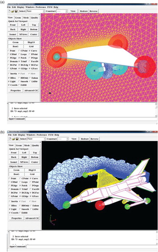
Figure 1 presents a flow chart of the developed simulation system for moving boundary problems. The first step adopts an in-house pre-processor named HEDP/Pre (HEDP: High End Digital Prototyping; Pre: Preprocessor) (Xie, Zheng, Chen, & Zou, 2008) to produce an initial grid. HEDP/Pre mainly adopts unstructured and hybrid grid generation techniques. It can be applied to mesh very complex aerodynamic configurations and provides user-friendly graphical user interfaces (GUIs) to visually steer the grid generation flowchart. Figure 2 shows two snapshots of the GUIs of HEDP/Pre, where the geometry is imported as a STEP (Standard for the Exchange of Product model data) file and represented by continuous surfaces; the surface and volume grids are then generated by a mapping-based advancing front mesher and a Delaunay mesher, respectively. Meanwhile, the grid sources are configured to refine the local grids where small element sizes are required for providing a better resolution for the geometrical and physical flow details.

Figure 1. Flow chart of the present simulation system for solving moving boundary problems.

Figure 2. Two snapshots of the GUIs of HEDP/Pre; the geometry models, grid sources, surface grids and initial volume grids (in 2D cut views) are presented for (a) the wing/pylon/store case and (b) the fully-loaded F16 aircraft simulation case.

The main loop of the developed simulation system includes four major steps:

1. Flow computation: Compute unsteady flows by using a finite volume solver.

2. Motion computation: Compute the aerodynamic forces and moments based on the flow simulation results, and use these as inputs to determine the positions of moving bodies in the next time step via the 6-DOF equations of motion.

3. Grid movement: Move the grid points accordingly to update the movement of the grid boundaries.

4. Local remeshing: If the grid movement yields elements of unacceptably poor quality, a hole is formed by deleting these elements and their neighboring elements, then a new grid is formed by merging the undeleted elements and newly-generated elements within the hole, and finally the solution is reconstructed by interpolating the results from the old grids onto the new grids.

This section reviews the technologies adopted in the first three steps. The improved local remeshing step is the main contribution of this study and is addressed in section 3. In section 4, the results from three main simulations are analyzed to verify the effectiveness and efficiency of the proposed approach using the configurations shown in Figure 2. Because many discussions in the following sections are based on these simulations, to present a better and clearer context, the computational conditions of these simulations are listed in Table 1, wherein the initial mesh sizes refer to the number of elements contained in the initial meshes.

Table 1. Computational conditions for the three store separation cases.

	Wing/pylon/store
Case	Case 1	Case 2	F16
Initial mesh size (million)	1.11/1.73	1.02	3.69
Mach number	1.20	0.95	1.2
Altitude (m)	11,600	7925	10,000
Angle of attack (°)	0		0
Mass (kg)	907		1800/317/317/231
Center of gravity (mm)	1417 (aft of store nose)		Midpoint of stores
Roll moment of inertia (kg·m^2)	27		110.25/4.85/4.85/4.30
Pitch moment of inertia (kg·m^2)	488		3500/125/125/258
Yaw moment of inertia (kg·m^2)	488		3500/125/125/258
Forward ejector location (mm)	1237.5 (aft of store nose)		Midpoint of stores
Forward ejector force (N)	10,700		211,951/37,327/37,327/27,200
Aft ejector location (mm)	1746.5 (aft of store nose)		–
Aft ejector force (N)	42,700		–
Ejector stroke length (mm)	100		–
Ejector stroke time of store Nos. 1, 2 and 4 (s)	–		0.000–0.054
Ejector stroke time of store No. 3 (s)	–		0.027–0.054

Note: The four stores involved in the fully-loaded F16 aircraft store separation case are numbered 1 to 4 from wing root to wing tip.

2.1. The CFD solver

With the development of an arbitrary Lagrangian–Eulerian (ALE) solution procedure in mind, the time-dependent compressible Navier–Stokes equations can be expressed as (1) where is the surface surrounding the control volume , is the outgoing unit vector normal to , is the vector of conservative variables, is the velocity of the surface, and and are the inviscid and viscous flux vectors, respectively.

The finite volume method is adopted to solve the Navier–Stokes equations. It considers as cell-averaged quantities and discretizes the Navier–Stokes equations in space as followins: (2) where the subscript represents the index of a face surrounding the control volume . It can be solved by the dual time-stepping method (Jameson, 1991). This method implies that Equation (2) is reformulated as a steady state problem at each time step. A variety of numerical schemes could then be used to solve this steady state problem. Here, we adopt the LU-SGS (Lower-Upper Symmetric Gauss-Seidel) scheme developed by Sharov and Nakahashi (1997).

To avoid the possible non-physical solutions due to the grid deformation, the change rate of element volume () and the velocities of element faces should satisfy the geometric conservation law (Thomas & Lombard, 1979), i.e., (3) where the gradient is computed by the Green–Gauss theorem and the flux is computed by the AUSM⁺-up Riemann solver (Liou, 2006). Meanwhile, the Venkatakrishnan’s limiter (Venkatakrishnan, 1993) is adopted to give the numerical scheme a monotone property.

The computational fluid dynamics (CFD) solver usually dominates the simulation cycle in terms of CPU time. To efficiently compute a flow problem that contains millions of grid points, the CFD solver has to be parallelized by subdividing the computational grid into several parts (Karypis & Kumar, 1998), solving the discretized equations on each part of the grid concurrently and communicating flow data shared by more than one process at domain interfaces using the message passing interface (MPI) library.

2.2. The solver for the 6-DOF equations of motion

Assuming that refers to the position vector of a point in the Cartesian coordinate frame fixed onto the rotating rigid body – i.e., the non-inertial reference frame (NIRF) – and refers to the origin of the NIRF in the inertial reference frame (IRF), the position , velocity and acceleration in the IRF can be written as (4)

The unconstrained motion of a rigid body can be described by Newton’s second law and the conservation law of angular momentum, i.e., (5) where is the mass of the rigid body, is the velocity of the center of gravity movement, is the total force acting on the rigid body, is the rotational angular velocity of the rigid body, is the rotational inertia tensor defined for the NIRF, and is the total moment about the body center of gravity. The equations can be solved by the fourth-order Runge–Kutta time integration, and the new position of any point on the rigid body can be obtained for the next time step simulation.

2.3. The grid deformation algorithm

In order to simulate the moving boundary problems, two types of grid deformation scheme prevail, which can be based on either an algebraic scheme (Liu et al., 2006; Morton, Melville, & Visbal, 1998; Sheng & Allen, 2013) or a physical-analogy technique (Blom, 2000; Clarence, 2004; Degand & Farhat, 2002; Karman, Anderson, & Sahasrabudhe, 2006; Stein, Tezduyar, & Benney, 2004; Sun, Zhang, & Ren, 2012; Zeng & Ethier, 2005; Zhou & Xu, 2010). The algebraic scheme defines the interior grid node movement as an algebraic function of the boundary node positions. In general, their computations are very efficient. However, because the algebraic functions are usually geometrically based and have little physical meaning, the control of the behavior of the grid deformation process by the algebraic scheme is often relatively weak and limited. In contrast, physical-analogy techniques such as the linear elastic technique (Karman et al., 2006; Stein et al., 2004) and the spring-analogy technique (Batina, 1991; Blom, 2000; Clarence, 2004; Degand & Farhat, 2002; Zeng & Ethier, 2005) provide the user with more flexibility to control the grid deformation by adjusting the physical parameters in an element-wise or edge-wise manner. For instance, badly-shaped elements can be more stiffened than those well-shaped elements to prevent the early appearance of an element with an unacceptable level of shape quality.

A study of the trade-off between flexibility and computational time (McDaniel & Morton, 2009) confirms the advantage of choosing the spring-analogy grid deformation technique, which treats each grid edge as a spring, thus making it possible to control the behavior of grid deformation by stiffening the grid edges individually. In the current implementation, the stiffness of a grid edge () with the two ending nodes and is expressed as (6) where is the length of the edge and is the minimum dihedral angle around the edge. According to Hook’s law, the initial force at the node is (7) where is the position vector of the node , is a set of nodes adjacent to the node , and is the size of the set . After allocating boundary points, the interior points need be arranged according to Equation (7). Here, the Jacobi iterative approach can be employed to compute the new positions of interior points: (8)

To reduce the computational cost, the number of iterations can be chosen as a smaller value than that required to achieve a real equilibrium status for Equation (7).

3. The local remeshing algorithm

In the case of large-scale boundary movements, the grid deformation algorithm may fail to produce a quality grid for the solver. Following each failure of the grid deformation step, a local remeshing algorithm must be employed to improve the robustness and quality of grid generation. In general, a remeshing algorithm takes the following steps:

1. Analyze the quality of the elements. If the grid has satisfactory quality for flow computation then advance to the next time step, otherwise determine the regions to be remeshed and extract their surface boundary information.

2. If the tetrahedral mesher employed for the remeshing process can manage a surface input with non-manifold edges then advance to the next step, otherwise enlarge the holes to ensure a manifold boundary.

3. Input the surface boundaries into a boundary constrained Delaunay mesher to generate new quality grids that fill in the holes and then replace the old grids with these new grids within the holes.

4. Reconstruct the solution by interpolating the most recent results onto the new grids and continue the flow computation.

3.1. Determination of regions to be remeshed

Different shape quality criteria have been proposed to assess the quality of a tetrahedral element in previous studies. The radius ratio , sliver value and skewness value are hereby selected to analyze the grid quality with the following equations: (9) (10) (11) where and are the radii of the inscribed and circumscribed spheres of the element, respectively, is the average length of the element edges, is the volume of the element, and is the volume of the ideal tetrahedron with an edge length of (12)

A tetrahedral element is identified as unqualified if its shape quality cannot meet predefined requirements, i.e., or or . Meanwhile, the proposed algorithm also checks the relative change of the value. A tetrahedral element is identified as unqualified as well if (13) where refers to the radius ratio of the element when it is created and is a threshold value set to be 0.85 as a default value.

If the current grid does not contain unqualified elements, the solution can be directly advanced to the next time step; otherwise, the following procedures are employed to determine the region to be remeshed:

1. All unqualified elements are marked as removable.

2. The elements neighboring the currently removable elements are marked as removable. Here, two elements are referred to as neighbors if they share at least one node point.

3. Repeat step (ii) two more times (therefore, step (ii) is executed three times in total).

Note that the initial holes formed in step (i) are usually too narrow to enable the generation of well-shaped elements inside the holes. Thus, in steps (ii) and (iii), the initial holes need to be enlarged by inserting more neighboring elements incrementally to ensure that the subsequent remeshing step can produce a quality grid. For simplicity, steps (ii) and (iii) together are referred to as the smoothing step hereafter.

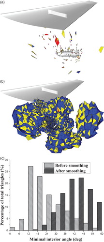
Figure 3 presents the hole regions before and after the smoothing step for the wing/pylon/store case study shown in Figure 2. In this case, the initial hole region is composed of 404 tetrahedra, and its boundary is composed of 1166 triangles. The hole region consists of many small holes (Figure 3(a)) – thus, it is impossible to produce a qualified grid for the next-step simulation by remeshing them. After the smoothing step, the enlarged hole region (Figure 3(b)) is composed of 154,739 tetrahedra, and its boundary is composed of 39,104 triangles. Consequently, the subsequent remeshing algorithm is able to produce good quality volume grids. Meanwhile, the smoothing step also provides a hole region with much better surface quality, which is beneficial for improving the element quality after the remeshing process. As shown in Figure 3(c), the minimal interior angles of less than 12° and 18° account for about 6.17% and 27.27% of the boundary triangles of the hole region before smoothing, respectively. The smoothing step removes all of the interior angles of less than 12° and outputs a hole region where only 0.38% of the boundary triangles have interior angles of less than 18°.

Figure 3. The influence of the smoothing step on the hole region: (a) the hole region before smoothing, (b) the hole region after smoothing, and (c) the distributions of the minimal interior angles of triangles that bound the hole regions before and after smoothing.

An important parameter (denoted by n_l) is defined as how many times the initial hole area should be enlarged by adding neighboring elements during the smoothing step. The determination of the value of n_l must consider two constrained goals of limiting the hole size and at the same time improving element quality after remeshing. We select the case shown in Figure 3 as an example and execute some numerical tests by increasing n_l from 0 to 6 to verify the above hole area determination algorithm. In the case of n_l = 6, the elements marked for removal account for about 43.8% of the entire meshes, and the region covered by these elements is denoted by Ω. Because a local remeshing algorithm is considered here, it is meaningless to let n_l be greater than 6. Then, we attempt to compare the quality of elements covering region Ω after the remeshing when n_l varies from 0 to 6, evaluated by the distribution of dihedral angles that are smaller than 15° (see Figure 4(a)). Note that the number of elements covering region Ω changes slightly with different values of n_l in this experiment. Therefore, it is fair to compare the number of dihedral angles directly. Meanwhile, Figure 4(b) lists how the number of elements marked for removal (denoted by n_rmv) changes against the value of n_l.

Figure 4. An experimental study on the impact of the number of times the initial hole is enlarged by adding neighboring elements in the smoothing step (denoted by n_l): (a) the distribution of small dihedral angles of elements created after remeshing compared to the value of n_l and (b) the number of elements filling up the holes before remeshing compared to the value of n_l.

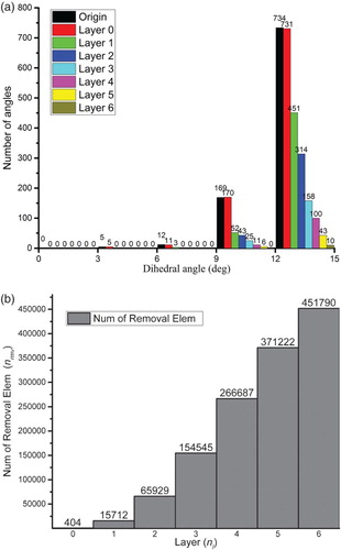
From Figure 4(a), we can see that the quality of elements covering region Ω after remeshing varies remarkably when the value of n_l increases. It is found that to avoid the generation of elements with angles less than 6°, the value of n_l must be greater than 1, and to avoid the generation of elements with angles less than 9°, the value of n_l must be greater than 2. The number of dihedral angles less than 12° decreases from 43 to 25 when the value of n_l increases from 2 to 3. As the value of n_l increases further, this number can be decreased because more stretched elements are removed and replaced by new elements with a better shape quality. However, a large value of n_l is not suggested here because the number of elements marked for removal almost doubles as the value of n_l increases from 3 to 4, while the improvement in element quality is marginal.

3.2. Suppression of non-manifold edges

The initial surface boundaries of the holes may contain non-manifold edges, and a considerable amount of coding effort may be required to enable an advancing front mesher or Delaunay mesher to manage a surface input with non-manifold edges. Although the in-house Delaunay mesher is able to treat such undesirable surface inputs, the current versions of tetrahedral meshers available in the public domain are likely to fail due to the presence of non-manifold edges. To facilitate the possible integration with such kinds of tetrahedral meshers, an algorithm is proposed here that can enlarge the holes so that their boundaries do not contain undesirable non-manifold edges. The example shown in Figure 5 is used to illustrate this algorithm. In this example, the elements abp₁p₂ (e₁) and abp₃p₄ (e₂) belong to the hole region. The notation ab is the common edge of elements e₁ and e₂ and is shared by four boundary faces of the hole region, i.e., p₁ab, p₂ab, p₃ab and p₄ab. To remove this non-manifold edge, the proposed algorithm takes the following steps:

1. Starting from element e₁, visit the elements adjacent to ab in a clockwise (or anti-clockwise) order until element e₂ is reached. The set of visited elements is denoted as E₁ (or E₂).

2. If E₁ is greater than E₂ then E = E₂, else E = E₁.

3. The holes are enlarged by inserting all elements within E.

Figure 5. An example illustrating the algorithm that removes non-manifold edges from the hole boundary by enlarging the hole region.

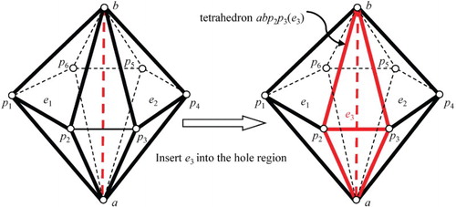
For the example shown in Figure 5, a manifold hole boundary is formed by inserting the tetrahedron abp₂p₃ (e₃) into the hole region. In the rare situations where new non-manifold edges are formed during the update of the boundaries of the holes, the above algorithm can be repeatedly called to remove all new non-manifold edges until a manifold hole boundary is produced. In practice, only a small number of elements are inserted into the holes due to the use of the above algorithm. For instance, the hole region shown in Figure 3(b) contains 128 non-manifold edges. After suppressing these edges, the number of tetrahedra contained in the hole region increase from 154,545 to 154,739, with only 194 additional tetrahedra being inserted during the process.

3.3. Local remeshing of the holes

3.3.1. The element scales.

The background grids represent one of the main approaches to encode a distribution of element scales in space. The element scale at any point can be computed by interpolating the scales defined at the corner nodes of a background cell containing this point. The main drawbacks of background grids are the memory cost associated with their construction and the man hours needed to build a good background grid for the manual case (Aubry, Dey, Karamete, & Mestreau, 2016; Aubry, Karamete, Mestreau, Dey, & Löhner, 2013). While the sources can be described through analytical functions, the distribution of element scales defined by sources is valid in the whole space. Therefore, a very complex sizing field may be obtained with only a few sources (Pirzadeh, 2010).

In this study, a few sources are used to control the spacing of the initial grid. Figure 6 illustrates the effect of a point source on the element spacing of its adjacent region. A point source is assigned with two radii and a spacing influence value. Within the inner radius, elements are generated that have a length scale similar to the spacing value specified. The element length scale then exponentially increases to a global spacing value outside the inner radius. The incremental rate of expansion of point spacing is defined by the relationship shown in Figure 6. This expression prescribes the spacing at the outer radius as twice that of the inner radius.

Figure 6. Illustration of the influence of a point source on the point spacing variation.

Moreover, more complex sources can be designed based on the point source, such as line sources and triangular sources. More details can be found in Zheng, Weatherill, and Turner-Smith (2002) on how to employ different types of grid source to facilitate the element spacing control of complex aerodynamics simulations.

In the remeshing phase, if only the boundary surface is input into a tetrahedral mesher then it may produce a much coarser volume grid than required, particularly in the case of remeshing a large-size hole. In commercial software such as ANSYS Fluent (Ansys, 2011), an approach based on background grids is employed to control the spacing of regenerated elements. In the present study, to reduce the computational time and memory costs associated with the background grid-based approach, and moreover, to be consistent with the aforementioned approach of initial grid generation, a moving-source approach is proposed for controlling the spacing of regenerated elements. To maintain a reasonable grid resolution after remeshing, the grid sources defined for initial grid generation are attached to geometric bodies accordingly. For example, while a body moves or rotates, the grid sources attached to this body also move the same distance or rotate at the same angle as the body itself. Despite its simplicity, this strategy can provide reasonable point distributions for local remeshing and thus ensure an acceptable level of simulation accuracy.

Figure 7(a) compares the variation of the number of volume elements (N_vol) with the body separation time for simulating the wing/pylon/store case in the mode of enabling or disabling the moving-source strategy. In the disabling mode, it was found that N_vol decreases slightly during the initial remeshing steps because at this stage the two separated bodies are very close to each other and the scales of regenerated elements are mainly determined by the scales of the surface elements of the bodies. This also explains the reasons why N_vol decreases much more sharply in the later remeshing steps, when the two bodies are far away from each other. After the remeshing step taking place at about t_s = 0.7 s, N_vol drops to 659,635, which is only about 60% of the total number of elements contained in the initial mesh, i.e., 1,111,001. This sharp drop in element number can have a marked effect on the simulation accuracy. In contrast, N_vol changes very smoothly in the enabling mode, fluctuating around its initial value. Although a drop is observed, the amount of variation is very small so that there is little impact on the simulation accuracy (see section 4 for more details).

Figure 7. The influence of the moving-source strategy on the magnitudes of the grids after each remeshing step: (a) the change curves of the number of volume elements in the mode of enabling or disabling the moving-source strategy, (b) a volume grid generated in the enabling mode, and (c) a volume grid generated in the disabling mode.

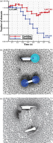
Figures 7(b) and 7(c) show two sets of volume grids that are generated in the enabling mode and disabling mode of applying the moving-source strategy, respectively. It is clearly shown that the grid generated in the disabling mode is much coarser than the grid generated in the enabling mode.

3.3.2. Tetrahedral grid generation

Given both the surface boundary of the hole region and the moved grid sources, a Delaunay mesher that respects the input boundary (Chen et al., 2011) is employed to remesh the hole region, and it takes the following main steps:

1. Construct an initial Delaunay tetrahedralization of the boundary points.

2. Recover boundary constraints by using the improved BR algorithm.

3. Insert field points with the modified Bowyer– Watson algorithm (George, 1997).

Note that the Delaunay tetrahedralization criterion provides a reasonable method for linking a given point set; however, it cannot ensure the existence of boundary constraints in the resulting tetrahedralization. Therefore, step (ii) is employed in the above remeshing process to recover the missing boundary entities from the Delaunay tetrahedralization of the boundary points.

Three-dimensional BR algorithms with theoretical proof of termination have been proposed when the insertion of Steiner points is allowed (Weatherill & Hassan, 1994). However, most of these BR algorithms can introduce an excessive number of Steiner points, in particular when the input surface contains a certain number of elements of high aspect ratio. In most cases, Steiner points degrade the robustness of the BR procedure because their positions are stored with floating-point numbers, which are essentially inaccurate due to round-off errors. Furthermore, Steiner points are harmful to element quality because they destroy local element size specifications and introduce elements with volumes close to zero. For moving boundary problems, grid faces are further stretched during the grid movement process, and some are located on the boundary of the hole region. Compared to the initial grid generation, local remeshing may sometimes provide even worse input data for the BR algorithm, and thus the usage of Steiner points can make resolving the robustness and element-quality issues an even more challenging task.

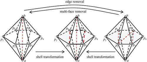
To resolve the above issues, a basic requirement is to reduce the usage of Steiner points in the BR procedure. To this end, a new boundary recovery scheme is proposed based on a novel flip operation, namely shell transformation. This scheme needs to be employed before the main BR procedure that considers how to recover boundary entities by inserting Steiner points (Chen et al., 2011; Du & Wang, 2004; George, Borouchaki, & Saltel, 2003; Weatherill & Hassan, 1994). Here, a shell refers to the region covered by a set of elements that meet at one common edge. The polyhedron shown in Figure 5 represents a typical shell, where the edge ab is the supporting edge, the nodes a and b are the supporting nodes, the nodes p_i (i = 1–6) are the skirt nodes, and the polygon p₁p₂ … p₆ is the skirt polygon. The boundary edges of the skirt polygon are the skirt edges (such as p₁p₂). Each skirt node and the supporting edge form a supporting face (such as abp₁). Each skirt node and either of the supporting nodes form a link edge (such as ap₁). Any valid mesh that covers a shell is called a covering mesh. The degree of a covering mesh refers to the number of elements that share the common supporting edge in this mesh. A shell is reduced if the degree of the new covering mesh is smaller than that of the old mesh. In particular, if the degree of the new mesh is zero, the shell is completely reduced; otherwise, the shell is partially reduced.

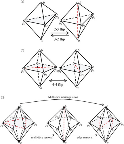
As shown in Figure 8, some flip operations are proposed to reconnect the grid topology of a shell, as seen in previous studies. Apart from the basic flips, i.e., 2-3, 3-2 and 4-4 flips (here the numbers denote the number of tetrahedra being removed and/or created by the flips, respectively; Joe, 1995), three advanced flips that involve more elements are suggested, i.e., edge removal (de l’Isle & George, 1995), multi-face removal (de Cougny & Shephard, 1995) and multi-face retriangulation (Misztal, Bærentzen, Anton, & Erleben, 2009). Note that the existing flips only consider grid configurations where skirt polygons are completely triangulated or untriangulated.

Figure 8. Existing flips for a tetrahedral mesh: (a) a 2-3 flip and 3-2 flip, (b) a 4-4 flip, and (c) multi-face removal, edge removal and multi-face retriangulation.

However, as shown in Figure 9, in the resulting grid after shell transformation, a core exists in the skirt polygon, referring to the unmeshed part of this polygon (note that the boundary nodes and edges of the core are called core nodes and core edges, respectively). In other words, shell transformation considers additional configurations where skirt polygons are partially triangulated. Therefore, shell transformation can not only represent the existing flips but is more likely to succeed because it attempts more possibilities for meshing a shell.

Figure 9. Illustration for the proposed shell transformation operation; the shell transformation considers all three of the mesh configurations shown in this figure, which correspond to three types of triangulation schemes for the skirt polygons: untriangulated (left), partially triangulated (middle) and completely triangulated (right).

Meanwhile, to overcome the limit of a single flip operation, we propose a way to employ shell transformation recursively. Considering the removal of an edge e in the grid, if the shell of e can only be partially reduced, the remaining supporting faces must be removed to reduce the shell further. Obviously, if either of the link edges that bound a supporting face f are removed then f will be removed as well. Assuming that the edge e₀ is picked for removal, shell transformation is called to reduce the shell of e₀. If the reduced shell of e₀ does not contain f and any new supporting faces sharing e, the shell of e is reduced as well; otherwise, a process that attempts to remove the supporting faces around e₀ is repeated. The above recursive routine can be employed not only to remove an edge directly but also to remove a face by attempting to remove any edge of that face. If an edge of the face is removed, the face will be removed as well.

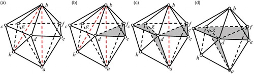
To help readers better understand this recursive scheme, Figure 10 illustrates its process operating on a local mesh composed of two shells (Figure 10(a)), aimed at removing the edge ab from the mesh. Firstly, shell transformation is called on the shell of ab. Since the shell cannot be completely reduced, ab still exists in the output mesh (Figure 10(b)). Nevertheless, the degree of the shell is reduced from 5 to 4. To reduce the shell further, the link edge bh is picked and shell transformation is called on the shell of bh, which reduces the shell completely. The degree of the shell of ab is reduced from 4 to 3 after this step (Figure 10(c)). Finally, shell transformation is called on the update shell of ab to remove ab using a single 3-2 flip (Figure 10(d); note that a 3-2 flip is a special case of shell transformation).

Figure 10. Illustration for the recursive scheme of shell transformation: (a) the input mesh, composed of two shells that are supported by the edges ab and bh, respectively, (b) the output after the first shell transformation calling on the shell of ab, (c) the output after the second shell transformation calling on the shell of bh, and (d) the final output after the third shell transformation calling on the shell of ab.

In this study, a BR scheme is developed to reduce the number of intersections between the boundary constraints and the grid entities by employing the recursive shell transformation routine. Taking the recovery of a boundary edge as an example, a boundary edge is lost because it intersects some grid edges or faces. If these intersecting entities are removed, the edge can be recovered as a result. Based on this idea, the recursive shell transformation routine can be employed to individually remove the grid edge or face that intersects the edge pending recovery.

The shell-transformation-based boundary recovery scheme attempts more possibilities to get an optimal grid of a shell (in this circumstance, a grid is said to be optimal when the grid intersects given boundary constraints the least); thus, it is more likely to succeed than other existing flip methods. Furthermore, shell transformation can be performed recursively to search for an optimal grid within a much larger grid space, where tens or even hundreds of shells are involved. Consequently, in all of the remeshing tests conducted so far, the improved BR algorithm can always recover all of the boundary constraints without using any Steiner points, and thus completely removes the adverse effects of Steiner points from the remeshing algorithm, improving robustness and element quality.

3.3.3. Grid quality improvement

In general, our algorithm executes the following types of local operation iteratively to remove badly-shaped elements:

1. Smoothing, which repositions mesh points to improve the quality of adjacent elements;

2. Point insertion/suppression, which improves a mesh by inserting a new point or removing an existing point;

3. Local reconnection, which replaces a local mesh with another mesh that fills up the same region. The new mesh has the same point set as the old mesh but with different point connections.

At present, the smoothing algorithm is based on the solution of a non-smooth optimization problem (Freitag & Ollivier-Gooch, 1997). The point suppression scheme is based on the edge-collapse operation (Klingner & Shewchuk, 2007). The local reconnection scheme adopts edge-removal and multi-face removal flips (see Figure 8(c)). With respect to point insertion, Klingner and Shewchuk (2007) suggest an effective but very time-consuming scheme that combines a Delaunay-type algorithm and smoothing operations. It is possible for hundreds of elements to be involved in just one single operation. Instead, we adopt an edge-splitting-based point insertion scheme that is more efficient and meets our goal of developing a cost-effective mesh improver for large-scale inputs.

3.4. Solution reconstruction by interpolation

After remeshing, the flow variable results in the remeshed region need to be transferred from the old grids to the new grids. Since the cell-centered method is adopted in the proposed CFD solver, the flow variables are defined at the centroid points of volume elements. To reconstruct the solution on the new grids, the most time-consuming step is finding a base element in the old grids that contains the centroid point of each element in the new grid. A standard strategy for speeding up this searching procedure is to set up some spatial decomposition structures such as octrees or alternative digital tree (ADTs). Alternatively, the present implementation makes the most of the spatial locality of the searching callings for different centroid points, i.e., the base elements for two geometrically neighboring positions are either similar or adjacent. Therefore, a walkthrough routine is developed to find the base element of a centroid point without the aid of any spatial decomposition structures. To be efficient, this routine needs to input a parameter that is a good initial guess for the base element.

To get good initial guesses for base elements, the elements in the new grid are classified as boundary or interior elements. A boundary element is adjacent to at least one boundary node of the holes, and an interior element has its four nodes newly inserted during the remeshing step. When searching for the base element of the centroid point of a boundary element (), the initial guess is specified as an element in the old grid that has one node common with , and this common node is exactly a boundary node of the holes that is adjacent to. After processing all of the boundary elements, a flood-fill-type algorithm can then be performed to treat the interior elements which ensures that, when searching through the base elements for an interior element (), the base element for one neighbor of must have been computed. Meanwhile, this base element for the neighbor is utilized as the initial guess of the base element for .

After determining the base element of a new element, the flow variable results defined at the base element are then transferred to the new element by a linear interpolation as (14) where and are the centroid points of the new element and the base element, respectively, is the existing flow value at the base element, is the flow value to be computed at the new element, and is the gradient of the existing flow value.

The process of computing the gradient defined on an element e takes three successive steps:

1. The physical value at each corner node of e is computed as the weighted sum of the values defined on the elements adjacent to this node. The weight for each element is inversely proportional to the distance between the corner node and the element center.

2. The physical value for each face () surrounding e is computed as the average of the values of its corner nodes.

3. The gradient defined on e can be computed by the Green–Gauss theorem: (15)

where V is the volume of e, refers to the outgoing unit vector normal to a face surrounding e, and is the area of the face.

4. Applications

As mentioned in section 2, a total of three simulations are conducted in this study to verify the effectiveness and efficiency of the developed simulation system. A full list of the computation conditions of these simulations is presented in Table 1. The first two simulations are based on the wing/pylon/store separation configuration (Figure 2(a)), where the focus is on the comparison of the simulation results of the developed system with wind-tunnel experimental data (Heim, 1991) and the results of commercial simulations (Snyder, Koutsavdis, & Anttonen, 2003) or in-house simulations (Biedron & Thomas, 2009; L. Zhang, Chang, Duan, Zhao, & He, 2012). The third simulation case is the store separation problem of a fully-loaded F16 aircraft (Figure 2(b)). Successful simulation of this case would demonstrate that the developed system is robust and applicable to the geometries of the type of complex flow problems that are experienced in industry.

4.1. The wing/pylon/store separation problem where Mach = 1.2

Figure 11 presents the contours of computed pressure distributions during the separation. The store moves slowly outboard in the z direction (Figure 11(a)). Meanwhile, the store pitches nose-up initially and then nose-down afterwards. In the x direction, the store moves rearward (Figure 11(b)).

Figure 11. Contour plots of the computed pressure distributions during the separation: (a) front view and (b) side view.

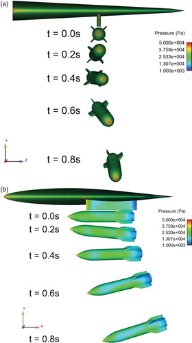
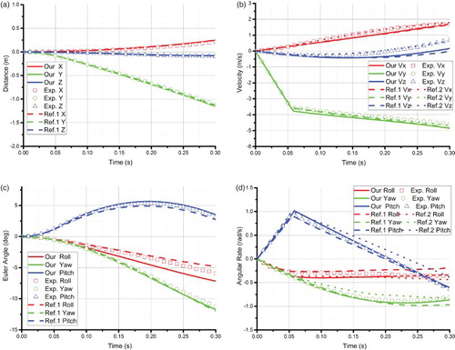
Figure 12 compares the present simulation results with the experimental data and the published numerical results. Figure 12(a) shows variation of the center of gravity (CG) of the store, evaluated in the global coordinate system, against the separation time t_s. It is shown that the present results agree very well with the experimental data. Meanwhile, the present CG results along the x direction are in better agreement with the experimental data than those published results, and this is also the case for the CG velocity data comparisons (Figure 12(b)). Note that in both the experiment and simulation scenarios, the store is clear of the ejectors after the separation distance is equal to 100 mm, which explains why a sudden change in velocity in the y direction is observed in all of the results at about t_s = 0.05 s (Figure 12(b)).

Figure 12. A comparison of the simulation results and experimental data vs. time for: (a) the store center of gravity, (b) the velocity of the store center, (c) the Euler angles, and (d) the Euler angular rates.

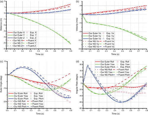
In addition, Figures 12(c) and 12(d) give the variations of the Euler angles and the Euler angular rates, respectively, against t_s. It is shown that the present pitch and yaw angles agree with the experimental data very well, as do the pitch and yaw rates. However, because the inertia moment along the roll axis is very small, the roll angle is very sensitive to accumulative errors in the predicted aerodynamics forces. Therefore, the roll angle diverges from the experimental results after t_s = 0.3 s (Figure 12(c)). This divergence is also observed in the numerical results of Snyder et al. (2003). Errors may also be partly due to the quasi-steady nature of the experiments. For the same reason, the present roll rate also diverges from the experimental data; nevertheless, the present rotation direction is always the same as that of the experimental data. In contrast, the rotation direction calculated by Snyder et al. (2003) somehow reverses after approximately t_s = 0.45 s (Figure 12(d)).

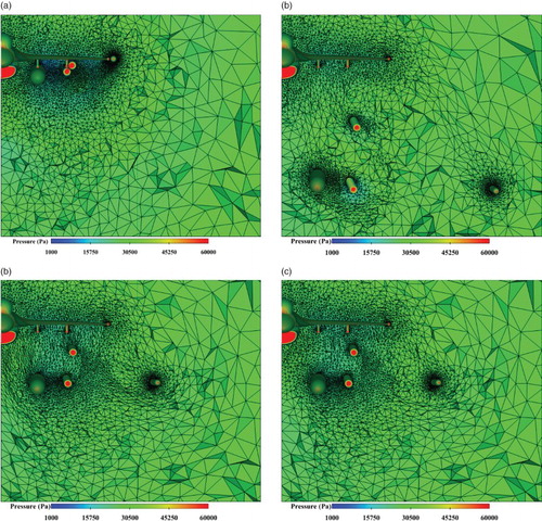
Apart from the simulation accuracy, the performance of the remeshing algorithm is another focus of this case study. Figures 13(a) and 13(b) show the initial volume grid and updated grid at t_s = 0.5 s. To illustrate the grid improvement effect of using the proposed remeshing algorithm more intuitively, Figures 13(c) and 13(d) present the grids before and after a local remeshing procedure at t_s = 0.38 s.

Figure 13. Cut views of the volume grids for the wing/pylon/store separation case at different times for: (a) t_s = 0.00 s, (b) t_s = 0.50 s, (c) t_s = 0.38 s before local remeshing, and (d) t_s = 0.38 s after local remeshing.

To demonstrate the benefits of the improved BR algorithm, a detailed comparison is presented for this simulation case between the Delaunay mesher proposed by Chen et al. (2011) (referred to as the old mesher hereafter) and the Delaunay mesher configured with the proposed BR algorithm (referred to as the new mesher hereafter). During this simulation, the remeshing algorithm is called 16 times in total by using the new mesher, and the performance data of the new mesher are collected in Table 2 (referring to those data before the forward slashes). Meanwhile, the old mesher is tested with the same inputs as those for the new mesher, i.e., 16 sets of surface grids defining the hole regions. Table 2 collects the performance data of the old mesher among its 16 runs for comparison (referring to those data after the forward slashes). The improved BR algorithm can always recover all of the boundary constraints without any Steiner points by employing shell-transformation-based mesh flip schemes. Not surprisingly, the old mesher cannot recover all of the boundary constraints by adopting the 2-3 and 3-2 flips (Chen et al., 2011). Thus, it is necessary to employ a very complicated procedure to recover those lost constraints further. This procedure requires the insertion of Steiner points into the surface boundaries for the conforming recovery of the prescribed constraints first, and then these points are moved into the domain interior for the constrained recovery second. Finally, an enhanced Steiner point suppression algorithm is employed to remove as many of these interior Steiner points as possible (Chen et al., 2011).

Table 2. Performance comparison of the Delaunay mesher proposed by Chen et al. (2011) (referred to as the old mesher) and the Delaunay mesher configured with the proposed BR algorithm (referred to as the new mesher).

Serial no.	1	2	3	4	5	6	7	8
Success	Y/Y	Y/Y	Y/Y	Y/Y	Y/Y	Y/Y	Y/Y	Y/Y
ncfm	0/348	0/416	0/936	0/1338	0/1828	0/3308	0/3575	0/3551
ncst	0/0	0/0	0/0	0/0	0/0	0/0	0/9	0/0
Total time (s)	3.20/6.00	4.90/8.90	4.30/14.80	13.20/28.20	17.50/43.60	15.90/96.70	19.80/108.00	17.00/106.00
Time for BR (s)	0.01/3.10	0.04/3.80	0.05/9.50	0.13/17.00	0.20/31.50	0.30/76.60	0.30/88.20	0.30/86.00
Min. angle (°)	16.5/15.0	15.2/15.9	15.1/12.6	15.0/15.9	14.4/14.4	10.4/9.5	13.3/4e−6	13.1/15.0
nlqe	35/15	14/20	37/64	28/35	56/86	90/11,9	96/11,00	95/10,8
Serial no.	9	10	11	12	13	14	15	16
Success	Y/Y	Y/N	Y/Y	Y/Y	Y/N	Y/Y	Y/Y	Y/Y
ncfm	0/4423	0/4487	0/2793	0/2100	0/2738	0/2389	0/2881	0/2882
ncst	0/0	0/	0/0	0/0	0/	0/0	0/0	0/0
Total time (s)	15.80/115.00	13.80/	21.60/99.80	15.50/77.80	10.10/	16.10/83.70	13.90/98.60	16.10/94.50
Time for BR (s)	0.30/94.70	0.17/	0.30/78.40	0.30/60.60	0.30/	0.30/68.40	0.20/80.20	0.20/77.80
Min. angle (°)	10.7/12.8	14.8/	14.8/15.0	15.5/13.3	13.7/	12.2/12.4	12.1/15.0	11.7/11.7
nlqe	86/133	66/	57/100	53/56	53/	42/67	80/67	44/54

Note: n_cfm = no. of Steiner points inserted for conforming recovery; n_cst = no. of Steiner points inserted for constrained recovery; n_lqe = no. of low-quality elements (referring to elements with angles smaller than 18°). The performance data of the new mesher and old mesher are placed before and after the forward slashes, respectively.

For the surface inputs mainly composed of well-shaped triangles, the old mesher usually inserts a small number of Steiner points in the conforming recovery step, and all of these points are then removed by the subsequent suppression algorithm. However, in the context of local remeshing, grid faces are stretched during the grid deformation process and some of them may appear on the boundaries of the holes to be remeshed. As a result, the old mesher always inserts an excessive number of Steiner points during the conforming recovery step (Table 2). The adverse effects of Steiner points on the remeshing processes in terms of robustness, efficiency and element quality are clearly evident:

1. Robustness: Presently, predicates such as those proposed by Shewchuk (1996) can enhance the robustness of BR remarkably. However, the positions of Steiner points stored with floating-point numbers are essentially inaccurate due to round-off errors, which can accumulate if an excessive number of Steiner points are inserted. Predicates using these positions as inputs may return an undesirable value and thus collapse the entire BR procedure. This accounts for two failures of the old mesher in this test case.

2. Efficiency: Among 14 successful runs of the old mesher, very time-consuming computations accompany the creation, movement and suppression of each Steiner point. This explains why the old mesher performs 1.8 to 7.3 times slower than the new one.

3. Element quality: Among 13 successful runs of the old mesher, its BR procedure achieved constrained recovery without inserting any Steiner points. In these cases, the quality of the grids created by the old mesher is comparable with those created by the new one. Nevertheless, in the remaining one successful run of the old mesher, its BR procedure achieved constrained recovery at the cost of inserting 9 Steiner points. These points are harmful to the final mesh quality because they may destroy the local mesh size specification and introduce elements with small volume sizes close to zero. Existing mesh improvement schemes may fail to remove all of the badly-shaped elements because many of them cluster in a local region where many Steiner points are located. The situation becomes even worse under the combined influence of Steiner points and badly-shaped boundaries. This explains why the grid created by the old mesher contains a number of elements with extremely small angles.

To demonstrate the capabilities of the developed system for viscous simulations, the viscous flow is simulated for this separation problem and the k-ω SST turbulence model is adopted in this simulation. Figure 14 presents the hybrid grids at different separation times. The initial grid is composed of about 798,074 prisms, 17,184 pyramids and 917,441 tetrahedra. Meanwhile, the simulation results are displayed in Figure 12 for comparison, together with the inviscid results and experimental data.

Figure 14. Cut views of the hybrid grids for the wing/pylon/store separation case at different times for: (a) t_s = 0.00 s, front view, (b) t_s = 0.00 s, side view, (c) t_s = 0.37 s before local remeshing, and (d) t_s = 0.37 s after local remeshing.

The roll angles and angular rates computed by the viscous simulation are in marginally better agreement with the experimental data than the inviscid results. The reasons why the improvements are not so evident deserve further investigations. It needs mentioning that, for the wing/pylon/store separation problem where Mach = 0.95 to discussed later in this paper, the roll angles and angular rates computed by a viscous simulation (L. Zhang et al., 2012) are also in marginally better agreement with the experimental data than the inviscid results computed by the proposed solver (Figures 15(c) and 15(d)). Meanwhile, because only the experimental data until t_s = 0.3 s are available in that case (while the experimental data until t_s = 0.8 s are available and used for comparison in this case), it is unclear whether or not the simulated roll angles and angular rates for the case where Mach = 0.95 after t_s = 0.3 s are in better agreement than their counterparts for the case where Mach = 1.2.

Figure 15. A comparison of the simulation results and experimental data vs. time for: (a) the store center of gravity, (b) the velocity of the store center, (c) the Euler angles, and (d) the Euler angular rates.

Note: Ref.1 = Zhang et al. (2012); Ref.2 = Biedron and Thomas (2009).

As shown in Figures 14(a) and 14(b), the initial boundary layer grid has to recede locally to leave enough space for the tetrahedra grid because of the narrow gap between the pylon and the store. In the separation process, the gap becomes larger and larger. However, because our local remeshing approach does not change the topology of the prisms and pyramids, no extra layers of boundary grid are created around the pylon and the store, meaning that the resolution of the boundary layer grid might be incomplete. A solution to this problem might be found in the local remeshing scheme proposed by Hassan, Sørensen, Morgan, and Weatherill (2007), which could propagate the boundary grid when necessary at each calling of local remeshing.

4.2. The wing/pylon/store separation problem where Mach = 0.95

To verify the computing accuracy of the developed system further, an experimental study (Heim, 1991) and two recent numerical studies on the wing/pylon/store separation problem where Mach = 0.95 were selected for comparison. The numerical study performed by L. Zhang et al. (2012) adopts a moving hybrid grid, while that performed by Biedron and Thomas (2009) adopts an overset moving unstructured grid. The comparison of the distance and Euler angle data does not involve the results by Biedron and Thomas (2009) because only the velocity and the Euler angular rate data are publically available.

It can be seen from Figures 15(a) and 15(b) that the position data and velocity data in both the x and y directions from the present simulation are in good agreement with the experimental data. However, the velocity data in the z direction computed by Biedron and Thomas (2009) are in better agreement with the experimental data, while the results of L. Zhang et al. (2012) and the present prediction are very close to each other. With respect to the angle data, L. Zhang et al. (2012) achieved more accurate roll angle predictions compared to the present study, and the yaw and the pitch angles computed by the two numerical schemes are in very good agreement with the experiment data (Figure 15(c)). Meanwhile, L. Zhang et al. (2012) show the most accurate roll angular rate predictions, while the present study achieved slightly better yaw angular rate predictions (Figure 15(d)).

In general, the above comparison reveals that the present numerical scheme can achieve a level of accuracy comparable with those recently published for this benchmark case. Nevertheless, it remains a challenge to simultaneously compute both the roll angles and the roll angular rates accurately.

To evaluate the computing efficiency of the procedures presented in this study, Table 3 lists a breakdown of the percentage of time spent on the different steps of the entire simulation cycle for this case study. The initial grid contains about 1.02 million tetrahedral elements. In this experiment, only the steps of the CFD solution and mesh deformation are executed in parallel on 32 computer cores, while other steps – including local remeshing – are executed sequentially. Not surprisingly, the CFD solution step is the most time-consuming, which used 93.1% of the total computing time. The mesh deformation step only used 3.8% of the total computing time because a simple spring-analogy approach was adopted. Although each local remeshing calling is not cheap, its total time cost is very low (using only 1.9% of the total computing time) because six callings is enough.

Table 3. A breakdown of the percentage of time spent on the different steps of the simulation cycle for the wing/pylon/store separation case where Mach = 0.95.

Step name	Time (s)	Percentage (%)
CFD solution	11,692.0	93.1
Mesh deformation	477.0	3.8
Local remeshing	243.6	1.9
Mesh gathering	20.2	–
Determining remeshing region	7.7	–
Delaunay meshing	10.3	–
Quality improvement	72.1	–
Solution reconstruction	90.6	–
Mesh repartitioning	42.7	–
Other	154.0	1.2
Total	12,566.6	100.0

It needs to be emphasized that the sequential local remeshing algorithm may become a major performance bottleneck when a much larger grid is required for the simulation and more computer cores are used for parallel CFD solution. In this case, a parallel scheme for local remeshing is indeed necessary (Chen, Li, Zheng, & Zheng, 2015; Tremel et al., 2007).

Convergence was determined by tracking the change in the residuals of the flow density during the solution. Figure 16 shows the residual changes with respect to iteration for the unsteady flow solution. At each time step, the residual drops down by about two orders. Following a local remeshing call, a sudden jump of the residual is observed at the same step. After this, the residual drops at the normal consistent rate when the solution advances continuously.

Figure 16. Residual versus iteration for the unsteady flow solution.

4.3. The store separation problem of a fully-loaded F16 aircraft

In order to verify the robustness of the developed system for complex simulations, the store separation process of a fully-loaded F16 aircraft was simulated. Four stores are separated from the aircraft in this test case. A full list of the computation conditions of this simulation is also presented in Table 1. Because no experimental data are available for the evaluation of the simulation results, the main focus is on the performance of the proposed remeshing algorithm. Compared with the wing/pylon/store separation cases, this simulation obviously involves more complicated geometric configurations and boundary movements, and thus challenges the proposed remeshing algorithm more extensively.

Figure 17 shows the cut views of the volume grids at different time steps. To refine the grids around the main body and the stores of the aircraft, a total of 84 grid sources are configured initially. During the store separation process, some of the grid sources attached to the stores are translated and rotated accordingly. Therefore, the grids around the moved stores are always reasonably well refined in the intermediate steps of the simulation. As a result, the amount of grids used in these intermediate steps is maintained at a level comparable with the initial volume grids. For instance, the volume grids shown in Figures 17(c) and 17(d) are composed of 3,306,643 and 3,306,682 elements, respectively. Note that keeping a reasonably consistent grid number is very important for a moving boundary simulation to achieve a balance in terms of accuracy and speed.

Figure 17. Cut views of the volume grids for the fully-loaded F16 aircraft store separation case at different times for: (a) t_s = 0.000 s, (b) t_s = 0.300 s, (c) t_s = 0.147 s before local remeshing, and (d) t_s = 0.147 s after local remeshing.

Because the simulation involves very complicated boundary movements, the proposed remeshing algorithm is employed very frequently. Considering the simulation process until t_s = 0.5 s, the remeshing algorithm is employed a total of 44 times. The improved BR algorithm is found to be key to the success of these remeshing callings, in which the boundary constraints are always recovered without any Steiner points. This observation is desirable because the performance of the remeshing step could be greatly improved after resolving the robustness, efficiency and element quality issues in relation to Steiner points.

5. Conclusion

An improved local remeshing algorithm has been proposed that addresses three important key issues. Firstly, a heuristic algorithm was developed to determine the remeshing region by expanding the initial hole composed of low-quality elements until a certain element quality can be reached after remeshing. The effect of the number of expansion cycles on the hole size and element quality after remeshing is experimentally analyzed, and a default value for this parameter is suggested. Meanwhile, a non-manifold hole can be transformed into a manifold one by adding adjacent neighboring elements into the hole. Secondly, a moving-source strategy was proposed to ensure a reasonable point distribution for the new grid that is used to fill in hole. Despite its simplicity, this strategy has proven to be very effective and can treat the moving boundary simulation to avoid potential unforeseen accuracy losses, while this strategy is disabled and a much coarser grid is created inside the hole. Thirdly, an improved boundary recovery procedure was proposed which ensures that the employed Delaunay grid generation approach can always create a new good-quality grid inside the hole without extremely badly-shaped elements and whilst respecting the precise hole boundary. This improved local remeshing algorithm has now been fully integrated with an in-house unstructured grid-based simulation system for solving moving boundary problems. The robustness and efficiency of the proposed local remeshing algorithm, together with the robustness and accuracy of the developed in-house simulation system, have been demonstrated through the performance of three challenging store separation simulations with complex geometries of a level that is experienced in industry.

Despite the achievements of this study, efforts are still necessary in order to further improve the developed simulation system. Hence, the following recommendations are made for future work:

1. The present software system can simulate unsteady viscous flows by moving boundary layer elements along with the rigid bodies surrounded by these elements. For viscous flow simulations involving boundary deformation, moving hybrid mesh techniques need be considered.

2. For the spring-analogy technique, we plan to consider using the torsional spring concept for further improvement in mesh deformation (Degand & Farhat, 2002).

3. Conservative interpolation schemes (Menon & Schmidt, 2011) need to be considered to replace the present non-conservative scheme.

4. Improving the flow solver by considering the global discrete geometric conservation law (Eken & Sahin, 2015) deserves further investigation.

Acknowledgements

The authors appreciate the constructive comments and suggestions made by the anonymous reviewers, which have been extremely valuable in significantly improving the quality of the manuscript. The second author acknowledges the joint support from Zhejiang University and the China Scholarship Council and the support received from Professors Oubay Hassan and Kenneth Morgan during his visiting research at Swansea University, UK. The fourth author acknowledges the Zhejiang Provincial HaiOu scheme in supporting his research visits to Zhejiang University.

Disclosure statement

No potential conflict of interest was reported by the authors.

Additional information

Funding

This work was supported by the National Natural Science Foundation of China [grant numbers 11172267, 11432013, 10872182, and 11272285]; and the Zhejiang Provincial Natural Science Foundation of China [grant numbers LR16F020002, Y1110038, and LQ14A020003].

References

- Ansys. (2011). ANSYS Fluent user’s guide. Release 14.0.
- Aubry, R., Dey, S., Karamete, K., & Mestreau, E. (2016). Smooth anisotropic sources with application to three-dimensional surface mesh generation. Engineering with Computers, 32(2), 313–330. doi:10.1007/s00366-015-0420-3
- Aubry, R., Karamete, K., Mestreau, E., Dey, S., & Löhner, R. (2013). Linear sources for mesh generation. SIAM Journal on Scientific Computing, 35(2), A886–A907. 10.1137/120874953
- Baker, T. J. (2003). Adaptive modification for time evolving meshes. Journal of Materials Science, 38(20), 4175–4182. doi:10.1023/A:1026385723850
- Batina, J. T. (1991). Unsteady Euler algorithm with unstructured dynamic mesh for complex-aircraft aerodynamic analysis. AIAA Journal, 29(3), 327–333. doi:10.2514/3.10583
- Biedron, R. T., & Thomas, J. L. (2009, January). Recent enhancements to the FUN3D flow solver for moving-mesh applications. Paper presented at the meeting of the 47th AIAA Aerospace Sciences Meeting Including the New Horizons Forum and Aerospace Exposition, Orlando, FL. AIAA 2009–1360. doi:10.2514/6.2009-1360
- Blom, F. J. (2000). Considerations on the spring analogy. International Journal for Numerical Methods in Fluids, 32(6), 647–668. http://dx.doi.org/10.1002/(SICI)1097-0363(20000330)32:6<647::AID-FLD979>3.0.CO;2-K
- Chen, J., Li, S., Zheng, J., & Zheng, Y. (2015, October). Parallel local remeshing for moving body applications. Research note presented at the meeting of the 24th International Meshing Roundtable, Austin, TX.
- Chen, J., Zhao, D., Huang, Z., Zheng, Y., & Gao, S. (2011). Three-dimensional constrained boundary recovery with an enhanced Steiner point suppression procedure. Computers and Structures, 89(5), 455–466. 10.1016/j.compstruc.2010.11.016
- Clarence, B. (2004, June–July). A robust unstructured grid movement strategy using three-dimensional torsional springs. Paper presented at the meeting of the 34th AIAA Fluid Dynamics Conference and Exhibit, Portland, OR. AIAA 2004–2529. doi:10.2514/6.2004-2529
- Compère, G., Remacle, J., Jansson, J., & Hoffman, J. (2010). A mesh adaptation framework for dealing with large deforming meshes. International Journal for Numerical Methods in Engineering, 82(7), 805–938. doi:10.1002/nme.2788
- de Cougny, H. L., & Shephard, M. S. (1995). Refinement, derefinement, and optimization of tetrahedral geometric triangulations in three dimensions. Unpublished manuscript. Rensselaer Polytechnic Institute, Troy, NY.
- Degand, C., & Farhat, C. (2002). A three-dimensional torsional spring analogy method for unstructured dynamic meshes. Computers and Structures, 80(3), 305–316. 10.1016/S0045-7949(02)00002-0
- de l’Isle, E. B., & George, P. L. (1995). Optimization of tetrahedral meshes. In I. Babuska, W. D. Henshaw, J. E. Oliger, J. E. Flaherty, J. E. Hopcroft, & T. Tezduyar (Eds.), Modeling, mesh generation, and adaptive numerical methods for partial differential equations (pp. 97–127). New York, NY: Springer.
- Du, Q., & Wang, D. (2004). Constrained boundary recovery for three dimensional Delaunay triangulations. International Journal for Numerical Methods in Engineering, 61(9), 1471–1500. doi:10.1002/nme.1120
- Eken, A., & Sahin, M. (2015). A parallel monolithic algorithm for the numerical simulation of large-scale fluid structure interaction problems. International Journal for Numerical Methods in Fluids. Advance online publication. 10.1002/fld.4169
- Freitag, L. A., & Ollivier-Gooch, C. (1997). Tetrahedral mesh improvement using swapping and smoothing. International Journal for Numerical Methods in Engineering, 40(21), 3979–4002. http://dx.doi.org/10.1002/(SICI)1097-0207(19971115)40:21<3979::AID-NME251>3.0.CO;2-9
- George, P. L. (1997). Improvements on Delaunay-based three-dimensional automatic mesh generator. Finite Elements in Analysis and Design, 25(3), 297–317. 10.1016/S0168-874X(96)00063-7
- George, P. L., Borouchaki, H., & Saltel, E. (2003). ‘Ultimate’ robustness in meshing an arbitrary polyhedron. International Journal for Numerical Methods in Engineering, 58(7), 1061–1089. doi:10.1002/nme.808
- Hassan, O., Probert, E. J., Morgan, K., & Weatherill, N. P. (2000). Unsteady flow simulation using unstructured meshes. Computer Methods in Applied Mechanics and Engineering, 189(4), 1247–1275. doi:10.1016/S0045-7825(99)00376-X
- Hassan, O., Sørensen, K. A., Morgan, K., & Weatherill, N. P. (2007). A method for time accurate turbulent compressible fluid flow simulation with moving boundary components employing local remeshing. International Journal for Numerical Methods in Fluids, 53(8), 1243–1266. doi:10.1002/fld.1255
- Heim, E. R. (1991). CFD wing/pylon/finned store mutual interference wind tunnel experiment. (AEDC-TSR-91-P4). Arnold AFS, TN: Arnold Engineering Development Center. Retrieved from http://oai.dtic.mil/oai/oai?verb=getRecord&metadataPrefix=html&identifier=ADB152669 (Last accessed on 23/3/2016)
- Jameson, A. (1991, June). Time dependent calculations using multigrid, with applications to unsteady flows past airfoils and wings. Paper presented at the meeting of the AIAA 10th Computational Fluid Dynamics Conference, Honolulu, HI. AIAA 91-1596. doi:10.2514/6.1991-1596
- Joe, B. (1995). Construction of three-dimensional improved-quality triangulations using local transformations. SIAM Journal on Scientific Computing, 16(6), 1292–1307. 10.1137/0916075
- Kannan, R., & Wang, Z. J. (2007). Overset adaptive Cartesian/prism grid method for stationary and moving-boundary flow problems. AIAA Journal, 45(7), 1774–1779. 10.2514/1.24200
- Karman, S. L., Anderson, W. K., & Sahasrabudhe, M. (2006). Mesh generation using unstructured computational meshes and elliptic partial differential equation smoothing. AIAA Journal, 44(6), 1277–1286. doi:10.2514/1.15929
- Karypis, G., & Kumar, V. (1998, November). Multilevel algorithms for multi-constraint graph partitioning. Paper presented at the meeting of the 1998 ACM/IEEE Conference on Supercomputing, San Jose, CA, 1–13. 10.1109/SC.1998.10018
- Klingner, B. M., & Shewchuk, J. R. (2007, October). Aggressive tetrahedral mesh improvement. Paper presented at the meeting of the 16th International Meshing Roundtable, Seattle, WA, 3–23. doi:10.1007/978-3-540-75103-8_1
- Liou, M. (2006). A sequel to AUSM, Part II: AUSM+-up for all speeds. Journal of Computational Physics, 214(1), 137–170. doi:10.1016/j.jcp.2005.09.020
- Liu, X., Qin, N., & Xia, H. (2006). Fast dynamic grid deformation based on Delaunay graph mapping. Journal of Computational Physics, 211(2), 405–423. 10.1016/j.jcp.2005.05.025
- Löhner, R. (1989). Adaptive remeshing for transient problems. Computer Methods in Applied Mechanics and Engineering, 75(1–3), 195–214. doi:10.1016/0045-7825(89)90024-8
- Löhner, R., Sharoy, D., Luo, H., & Ramamurti, R. (2001, July). Overlapping unstructured grids. Paper presented at the meeting of the 39th AIAA Aerospace Sciences Meeting and Exhibit, Reno, NV. AIAA 01-0439. 10.2514/6.2001-439
- McDaniel, D. R., & Morton, S. A. (2009, January). Efficient mesh deformation for computational stability and control analyses on unstructured viscous meshes. Paper presented at the meeting of the 47th AIAA Aerospace Sciences Meeting Including the New Horizons Forum and Aerospace Exposition, Orlando, FL. AIAA 2009–1363. 10.2514/6.2009-1363
- Menon, S., & Schmidt, D. P. (2011). Conservative interpolation on unstructured polyhedral meshes: An extension of the supermesh approach to cell-centered finite-volume variables. Computer Methods in Applied Mechanics and Engineering, 200(41), 2797–2804. 10.1016/j.cma.2011.04.025
- Misztal, M. K., Bærentzen, J. A., Anton, F., & Erleben, K. (2009, October). Tetrahedral mesh improvement using multi-face retriangulation. Paper presented at the meeting of the 18th International Meshing Roundtable, Salt Lake City, UT, 539–555. doi:10.1007/978-3-642-04319-2_31
- Morton, S. A., Melville, R. B., & Visbal, M. R. (1998). Accuracy and coupling issues of aeroelastic Navier-Stokes solutions on deforming meshes. Journal of Aircraft, 35(5), 798–805. doi:10.2514/2.2372
- Pirzadeh, S. Z. (2010). Advanced unstructured grid generation for complex aerodynamic applications. AIAA Journal, 48(5), 904–915. doi:10.2514/1.41355
- Prewitt, N. C., Belk, D. M., & Shyy, W. (2000). Parallel computing of overset grids for aerodynamic problems with moving objects. Progress in Aerospace Sciences, 36(2), 117–172. doi:10.1016/S0376-0421(99)00013-5
- Sharov, D., & Nakahashi, K. (1997, June–July). Reordering of 3-D hybrid unstructured grids for vectorized LU-SGS Navier-Stokes computations. Paper presented at the meeting of the 13th Computational Fluid Dynamics Conference, Snowmass Village, CO, 2102–2117. AIAA 97-2102. doi:10.2514/6.1997-2102
- Sheng, C., & Allen, C. B. (2013). Efficient mesh deformation using radial basis functions on unstructured meshes. AIAA Journal, 51(3), 707–720. doi:10.2514/1.J052126
- Shewchuk, J. R. (1996, May). Robust adaptive floating-point geometric predicates. Paper presented at the meeting of the 12th Annual Symposium on Computational Geometry, Philadelphia, PA, 141–150. doi:10.1145/237218.237337
- Si, H., & Gärtner, K. (2011). 3D boundary recovery by constrained Delaunay tetrahedralization. International Journal for Numerical Methods in Engineering, 85(11), 1341–1364. doi:10.1002/nme.3016
- Snyder, D. O., Koutsavdis, E. K., & Anttonen, J. S. (2003, June). Transonic store separation using unstructured CFD with dynamic meshing. Paper presented at the meeting of the 33rd AIAA Fluid Dynamics Conference and Exhibit, Orlando, FL. AIAA 2003–3919. doi:10.2514/6.2003-3919
- Stein, K., Tezduyar, T. E., & Benney, R. (2004). Automatic mesh update with the solid-extension mesh moving technique. Computer Methods in Applied Mechanics and Engineering, 193(21), 2019–2032. doi:10.1016/j.cma.2003.12.046
- Sun, X., Zhang, J., & Ren, X. (2012). Characteristic-based split (CBS) finite element method for incompressible viscous flow with moving boundaries. Engineering Applications of Computational Fluid Mechanics, 6(3), 461–474. 10.1080/19942060.2012.11015435
- Thomas, P. D., & Lombard, C. K. (1979). Geometric conservation law and its application to flow computations on moving grids. AIAA Journal, 17(10), 1030–1037. 10.2514/3.61273
- Togashi, F., Nakahashi, K., Ito, Y., Iwamiya, T., & Shimbo, Y. (2001). Flow simulation of NAL experimental supersonic airplane/booster separation using overset unstructured grids. Computers and Fluids, 30(6), 673–688. 10.1016/S0045-7930(00)00033-5
- Tremel, U., Sørensen, K. A., Hitzel, S., Rieger, H., Hassan, O., & Weatherill, N. P. (2007). Parallel remeshing of unstructured volume grids for CFD applications. International Journal for Numerical Methods in Fluids, 53(8), 1361–1379. 10.1002/fld.1195
- Venkatakrishnan, V. (1993, January). On the accuracy of limiters and convergence to steady state solutions. Paper presented at the meeting of the 31st AIAA Aerospace Sciences Meeting and Exhibit. Reno, NV. AIAA 93–0880. doi:10.2514/6.1993-880
- Wang, Z. J., & Parthasarathy, V. (2000). A fully automated Chimera methodology for multiple moving body problems. International Journal for Numerical Methods in Fluids, 33(7), 919–938. http://dx.doi.org/10.1002/1097-0363(20000815)33:7<919::AID-FLD944>3.0.CO;2-G
- Weatherill, N. P., & Hassan, O. (1994). Efficient three-dimensional Delaunay triangulation with automatic point creation and imposed boundary constraints. International Journal for Numerical Methods in Engineering, 37(12), 2005–2039. doi:10.1002/nme.1620371203
- Xie, L., Zheng, Y., Chen, J., & Zou, J. (2008). Enabling technologies in the problem solving environment HEDP. Communications in Computational Physics, 4(5), 1170–1193.
- Zeng, D., & Ethier, C. R. (2005). A semi-torsional spring analogy model for updating unstructured meshes in 3D moving domains. Finite Elements in Analysis and Design, 41(11), 1118–1139. doi:10.1016/j.finel.2005.01.003
- Zhang, L., Chang, X., Duan, X., Zhao, Z., & He, X. (2012). Applications of dynamic hybrid grid method for three-dimensional moving/deforming boundary problems. Computers and Fluids, 62, 45–63. 10.1016/j.compfluid.2012.03.008
- Zhang, Z., Gil, A. J., Hassan, O., & Morgan, K. (2008). The simulation of 3D unsteady incompressible flows with moving boundaries on unstructured meshes. Computers and Fluids, 37(5), 620–631. 10.1016/j.compfluid.2007.07.013
- Zheng, Y., Weatherill, N. P., & Turner-Smith, E. A. (2002). An interactive geometry utility environment for multi-disciplinary computational engineering. International Journal for Numerical Methods in Engineering, 53(6), 1277–1299. doi:10.1002/nme.288
- Zhou, X., & Xu, H. (2010). Gridless method for unsteady flows involving moving discrete points and its applications. Engineering Applications of Computational Fluid Mechanics, 4(2), 276–286. doi:10.1080/19942060.2010.11015316