Comment on the level-set method used in ‘Numerical study on mobilization of oil slugs in capillary model with level set approach’

ABSTRACT

This is a comment on a 2014 paper by Dai and Wang. It is argued that the validation in Dai and Wang's paper is an artifact caused by the boundary conditions of the level-set function, meaning that the effects reported in their paper have little physical relevance. Simulations are presented using Dai and Wang's methods to illustrate this claim. Remarks are made on the choice of boundary conditions for the level-set function, as well as the frequency of reinitialization, both of which are important topics that are sometimes overlooked. A simple criterion is proposed for determining the appropriate reinitialization frequency in simulations of highly viscous flows.

KEYWORDS:

• Level-set method
• axisymmetric flow
• two-phase flow
• projection method
• water film
• oil slug mobilization

1. Introduction

The application of computational fluid dynamics (CFD) to engineering problems yields valuable insight into a wide range of phenomena, but there are many pitfalls that may render the results invalid. When writing and using in-house code, these pitfalls increase in number – but fortunately there are several tools available to the CFD practitioner which can help to avoid them. Verification and validation are key concepts in this context. When a simulation attempts to capture a wide range of physical phenomena, such as in two-phase flow simulations with contact lines, there are many effects – both numerical and physical – which affect the result. When these effects are similar in appearance, the validation of the code becomes even more difficult.

A third concept that is of fundamental importance in all of science is that of reproducibility. The rapid development of computational methods means that much effort is needed to reproduce a result that uses many complicated methods. In this particular case, it is extraordinarily fortunate that it is possible to reproduce and make comments on the results of Dai and Wang (2014), since in-house Fortran code that already has the methods they implemented is available.

Dai and Wang (2014) concerns the mobilization of oil slugs in capillaries. The physics of this interesting phenomenon are not discussed here; the reader is referred to Morrow and Mason (2001) for a review of the importance of oil slugs in capillaries to the recovery of crude oil, and to Mumley, Radke, and Williams (1986) for a review of liquid–liquid flows in glass capillaries, which can be used as a model system.

The paper is organized as follows. In the next section, the content of Dai and Wang (2014) is summarized. Section 3 presents a brief review of the computational methods used, then section 4 argues the case that the validation in Dai and Wang , as well as some of the physical interpretations, is based on numerical artifacts. It is also pointed out that an essential physical effect, the Navier slip at the contact line, does not seem to be taken into account. Section 5 presents remarks on the topics of boundary conditions for the level-set method and reinitialization frequency, and section 6 concludes the paper.

2. Summary of Dai and Wang (2014)

Dai and Wang (2014, p. 1) describe their work as a ‘numerical investigation on mobilizing oil slugs trapped in an axisymmetric capillary tube saturated with water’. They employ a level-set method for interface tracking, together with the popular Chorin projection method for solving the incompressible Navier–Stokes equations in a relatively fast way, and they use the continuum surface force (CSF) method to handle the variations in density and viscosity and the surface tension between the two phases.

Using this method, they find that a thin film of water coats the capillary tube, a phenomenon which is also seen in experiments. They compare the dimensions of this thin film with the experimental values and find reasonable agreement. They then proceed to consider phenomena that occur later in the time evolution of the slug, and propose explanations of these based in part on the properties of the thin film.

3. Methods

The numerical methods used in Dai and Wang (2014) are now briefly outlined. On the few points where the description in Dai and Wang is not detailed enough for a full reproduction, the assumptions made in this paper about what Dai and Wang used are stated. It is accepted that it is infeasible to completely describe a numerical code of this size in a publication, so this is not a criticism about the level of detail provided in Dai and Wang, just a point of clarification for the purposes of this paper. As in Dai and Wang, in-house Fortran code was used to implement the methods described here. This code has been validated and applied to various physical phenomena (e.g. Ervik, Lervåg, & Munkejord, 2014; Teigen, Lervåg, & Munkejord, 2010; Teigen & Munkejord, 2009, 2010). A complete description of the algorithm and numerical methods can be found in Teigen(2010, ch. 2).

The projection method (Chorin, 1968) is employed for solving the incompressible Navier–Stokes equations: (1) (2) where is the velocity field, ρ is the density, μ is the dynamic viscosity, p is the pressure, is a body acceleration (force per density) such as gravity and is a singular acceleration term arising in the case of two-phase flow. The projection method eliminates Equation (1(1) ) and introduces a Poisson equation that must be solved for the pressure, p, at each time step, given the velocity field at the previous time step.

The equations are discretized in space on a structured, uniform, staggered and Cartesian grid using the finite-difference method. For the temporal discretization, an explicit Runge–Kutta (RK) method is used. A second-order strong stability-preserving RK method is applied here (Gottlieb, Ketcheson, & Shu, 2009). The overall scheme is however limited to the first order in time due to the irreducible splitting error arising from the projection method (for a thorough review, see Guermond, Minev, & Shen, 2006). For the discretization in space, a second-order essentially non-oscillatory (ENO) scheme (Shu & Osher, 1988) is employed for all spatial derivatives, except for the discretization of the viscous terms in the Navier–Stokes equation, where the standard central difference scheme is used. This is the same approach as used in Dai and Wang (2014).

The solution of the discretized Poisson equation is the most time-consuming step in such a solver, and much work has gone into the development of fast solvers for this equation. As the discretized Poisson equation arising from axisymmetric two-phase flow is non-symmetric and quite ill-conditioned, a direct method is preferable to an iterative one in the case where the mesh is small enough for a direct method to be feasible. Here the mesh size is indeed manageable, so the direct method of lower-upper factorization is used, for which the portable extensible toolkit for scientific computing (Balay, Gropp, McInnes, & Smith, 1997) library is employed. Dai and Wang (2014) do not specify the method they used to solve the Poisson equation, but as the mesh becomes further refined, iterative methods in general – and multigrid methods in particular – become superior to direct solvers.

When extending this to two-phase flow, two main ingredients are needed: information about the position of the interface, and a method to handle the varying density, viscosity and surface tension. In Dai and Wang (2014), the level-set method (Osher & Fedkiw, 2001; Osher & Sethian, 1988) and the continuum surface force (CSF) method (Brackbill, Kothe, & Zemach, 1992) are employed, and so the very same methods are used in the present paper. The CSF method handles the difference in viscosity, density and surface tension by using a singular acceleration term (as outlined in Equation (2(2) )), which is subsequently smeared out to the grid points by means of a mollified δ-function (Brackbill et al., 1992).

The level-set method is an interface-capturing method where the interface is represented by a Eulerian field φ defined in the entire domain. This field φ is advected directly, and the interface is found as the zero-level set of φ, hence the name. A common choice for φ is that of a signed distance function having . This property is in general not preserved under the advection of φ, leading to the use of reinitialization, meaning that φ is periodically reconstructed to obtain whilst preserving the location of the zero-level set. The ENO discretization is used both in the level-set advection and the reinitialization equations, together with the second-order strong stability-preserving-RK method. As has been noted by several authors (e.g. see Hartmann, Meinke, & Schröder, 2010), reinitialization does not preserve the interface location exactly, and its too-frequent application may result in a loss of accuracy and numerical artifacts, as will be seen in subsequent sections of this paper.

Finally, it is noted that the time step in the aforementioned RK method is restricted in the case of two-phase flow by the smallest of several Courant-Friedrichs-Lewy (CFL) conditions, namely one based on convection, one based on the viscous term, and one based on the surface tension. In particular, the viscous CFL condition takes the form (3) where C is a constant and is the kinematic viscosity. This can be very restrictive indeed when simulating a creeping flow on a fine mesh (for a detailed account of the various CFL conditions, see Kang, Fedkiw, & Liu, 2000).

4. Arguments regarding validation and physical interpretation

It is noted that Dai and Wang (2014) use the word ‘verification’ for what is termed ‘validation’ in this paper. Here, the definition in Oberkampf and Trucano (2002) is followed, and the validation performed in section 6 of Dai and Wang is considered from this perspective. To restate the case definition of Dai and Wang: an oil slug is initially placed at rest in a capillary tube with an inner diameter of 2 mm. This slug is surrounded by water, and mobilized by an inflow of water at one end of the capillary, at a flow rate of 0.01 m/s. Since this case is axisymmetric, a 2D axisymmetric coordinate system is used.

In Dai and Wang (2014) the formation of a water film between the oil slug and the domain edge (capillary wall) is observed. The authors present a table showing the thickness of this water film for three different mesh resolutions. This table is reproduced in Table 1 in the present paper, which also shows the grid spacing for comparison. As is evident from Table 1, the water film is resolved by approximately one grid cell, and so the claims that important physical effects arising from this water film are captured by the numerical simulations seem to be without support. The mere fact that the film thickness has stagnated between the last two grid resolutions does not indicate convergence, since the convergence of a calculated property under grid refinement cannot be expected to be monotonous and smooth (for an example of non-monotonous convergence under grid refinement, see Eça & Hoekstra, 2009, Figure 5). No further attempts at validation are made by Dai and Wang.

Table 1. Comparison of the film thicknesses and mesh resolutions used for validating the cases in Dai and Wang.

Mesh	Film thickness

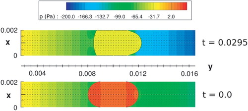
Having considered this, Dai and Wang (2014) continue to interpret various effects that the oil film has on the system. As an example, they consider the effect on the pressure drop across the oil slug (Figures 5 and 7 in their paper) which relies on a correlation in time between the thickness of the numerical oil film and the change in the shape of the interface. As the water film appears to be a numerical artifact, an alternative physical explanation is put forward in the present paper – namely that the product of surface tension and curvature, , gives the well-known Laplace pressure difference across an interface. For the initial condition of an oil slug with two hemispherical ends, the two pressure jumps across the two interfaces that are encountered when traversing the length of the tube cancel each other out. When the slug starts moving, the rear end becomes flattened while the front end still has a significant curvature, so is larger at the front than at the back. This gives rise to the increase in pressure difference that is in Figure 5 of Dai and Wang, and is illustrated further in Figure 1 of the present paper.

Figure 1. The pressure and velocity fields shown at t=0.0 s (bottom) and t=0.0295 s (top).Note: It is seen that the changes in the curvature of the rear end of the oil slug are a plausible explanation for the increase in the pressure drop. This plot is from the simulations conducted in the present paper.

Finally, there is another effect that must be taken into account for a realistic simulation of the mobilization of oil slugs in capillaries. If the drop is to move along the capillary surface, the contact line between the oil, the water and the capillary must also move. It is known that this is incompatible with the standard no-slip boundary condition for the flow field, since the stress at the boundary becomes infinite (Navier, 1823). The standard approach is to use the Navier slip condition (e.g. see Ding & Spelt, 2007) with some empirical relation for the slip velocity (e.g. see the discussion in Chandra & Batur, 2010). The slip is unrelated to the level-set approach, but must be incorporated into the flow solver; however, the slip may depend on the contact angle computed from the level-set function. It does not appear that this is taken into account in Dai and Wang.

5. Remarks on boundary conditions and reinitialization frequency

As mentioned in the introduction, boundary conditions for φ and the reinitialization frequency are sometimes overlooked in the literature on level-set methods, and the present case is a good example with which to illustrate this.

On the first point of boundary conditions for the level-set function, there is a recent paper by Della Rocca and Blanquart (2014) which has a thorough discussion of various methods. The novel method proposed in Della Rocca and Blanquart is a modification to the standard reinitialization equation in the vicinity of a boundary, which the authors compare to existing approaches, such as the one used in both the present paper and Dai and Wang (2014). The method proposed by Della Rocca and Blanquart appears to be very promising, as well as simple to implement, so it is recommended for contact line applications such as the case of capillary slug flow discussed here. Setting this method aside, the two simplest boundary conditions for φ are the zero-Neumann boundary condition and the extrapolation of φ outwards from the domain interior. The effects of choice of boundary condition is illustrated in Figure 2. Extrapolation here means that the values of φ outside the domain are set as , where is the value at the grid point that is next to the boundary, and is the value at that is located one grid point further into the domain. See also the illustration in Figure 3(c). Dai and Wang do not mention what method they use, but it is demonstrated in this paper that it could not have been the zero-Neumann condition, which leaves extrapolation.

Figure 2. Comparison of the two boundary conditions for the level-set function φ: (a) the zero-Neumann boundary condition and (b) the extrapolation of φ.Note: Both figures are snapshots of the leading edge of the slug at t=0.005 s. The color indicates the pressure field, and the vectors show the velocity field at every fifth point in the x- and y-directions. This plot is from simulations conducted in the present study.

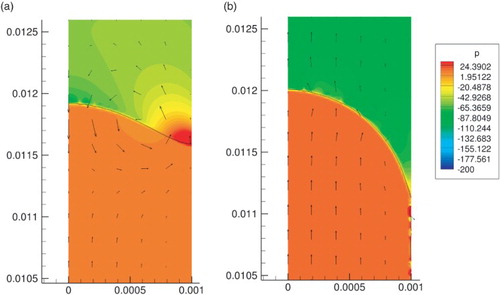
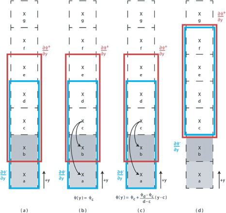
Figure 3. Illustration of the feedback loop that gives rise to the numerical oil film.Note: Figure reprinted from Della Rocca and Blanquart (2014) with permission from Elsevier.

To illustrate the difference between these two choices, the slug flow in a capillary with a 2-mm diameter and an injection rate of 0.01 m/s was computed, shown here at t=0.005 s in Figure 2. The pressure field (color), the interface position and the velocity vectors (at every fifth point) are all shown. It can be seen in Figure 2(a) that the zero-Neumann boundary condition drives the interface towards being normal to the boundary, and in the process introduces an unphysical capillary wave which affects the rest of the interface. The end result is that of a flat interface at both edges of the slugs. Thus the zero-Neumann boundary condition is clearly not useful in this case. This is also reported, for example, in Della Rocca and Blanquart (2014, section 3.3.1).

The second option, extrapolation, is seen in Figure 2(b) to give a much more reasonable-looking result. Indeed, it can even be seen that the water film along the domain edge reported in Dai and Wang (2014) has started forming. Alas, as is now illustrated, this is a purely numerical artifact caused by the reinitialization procedure. Turning again to Della Rocca and Blanquart (2014), the cause of the artifact may be understood through the examination of Figure 6 in their paper, reproduced here as Figure 3, wherein the various boundary conditions and stencils are shown schematically.

In Figure 3(c), the extrapolation procedure is illustrated. It can be observed that the extrapolation provides the values of φ at the points labeled a and b by using the values at points c and d. When performing the reinitialization and using the ENO stencil, the values at points c and d are computed using (amongst others) the values at points a and b. But these were first calculated from the original values at points c and d, so this introduces a feedback loop. It can be shown that this feedback drives the contact angle to 0 for obtuse points (Della Rocca & Blanquart, 2014).

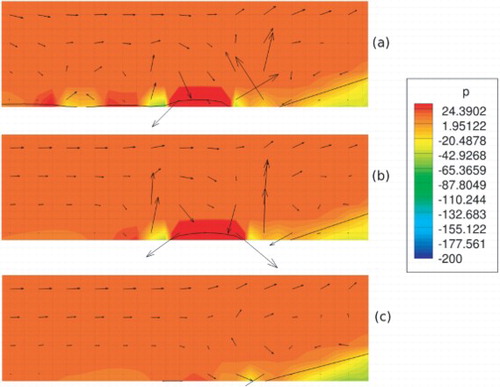
A second point regarding the reinitialization frequency is that a balance must be struck between the loss of accuracy caused by reinitialization occurring too frequently and the loss of accuracy caused by reinitialization occurring too infrequently. The two extremes in this regard consist in never reinitializing φ and reinitializing φ every time step (or even every substep employed in the time integration of the velocity field). From the algorithm described in Figure 2 of Dai and Wang (2014), it can be seen that they have used the latter approach, namely reinitializing every time step. That the reinitialization frequency has a significant impact in this instance is demonstrated in Figure 4 of the present paper, wherein the case used in Dai and Wang is simulated with different reinitialization frequencies and a close-up around the contact point at s is shown. It can be seen that reducing the reinitialization frequency delays the film formation.

Figure 4. The effect of reinitialization frequency on the development of the thin film around the leading contact point for reinitialization occurring (a) every time step, (b) every 5 time steps and (c) every 20 time steps.Note: A close-up is shown of the contact point at t=0.005 s. These plots are from simulations conducted in the present study.

As a final remark on this point, it is noted that the combination of two well-known facts gives a simple method for determining a lower bound on the reinitialization frequency. The first is that reinitialization of the level-set function is introduced in order to correct deviations from a signed distance function that arise when the field φ is advected. The second is that in cases where creeping flow is simulated using an explicit time integration method, such as here, the time step is determined by the viscous CFL criterion, which is more stringent than the convective CFL criterion. As an example, in the case considered here, the viscous CFL criterion as computed from Equation (3(2) ) is roughly 175 times more restrictive than the convective time step.

It thus follows that reinitialization should not be performed every time step when simulating creeping flow, since this constitutes an overcorrection, which is known to lead to accumulating errors (e.g. see Hartmann et al., 2010). It is postulated that a good solution is to use the convective time step to determine the correct frequency. Since the convective time step is smaller than the time it takes for a fluid particle to cross a grid cell, it must take longer than this time step for φ to be significantly distorted by advection. It follows that reinitializing every convective time step is better than reinitializing every time step for a creeping flow. Note that for a non-creeping flow, this solution reduces to the standard method, so it may be applied in all cases. Note also that this solution will only reduce the computation time, since it requires less operations than the standard method – but the improvement is not expected to be significant, since the projection method dominates the time consumption.

To the author's knowledge, this simple improvement has not been suggested elsewhere in the literature on reinitialization. As has been illustrated and discussed, the case of oil slug flow considered here needs an improved boundary condition for φ – such as that proposed by Della Rocca and Blanquart (2014) – and an implementation of the Navier slip condition in order to be physically relevant. Therefore, the testing of this proposed improvement is left as a topic for future work.

6. Conclusions

This paper has presented a brief summary of Dai and Wang (2014) and commented on the validation performed in that paper which is centered around the observation of a thin water film. It has been argued that this water film is a numerical artifact arising from the boundary conditions used when reinitializing the level-set function. Having tested the two simple boundary conditions that are most commonly used, it appears that extrapolation was used in Dai and Wang, and thus the same method is also used in the present paper. An alternative physical explanation of the time variation in the pressure drop along the oil slug has been offered, namely that it is caused by the change in the shape of the head and the tail. It has been noted that a realistic simulation of oil slug flow should also take into account the contact angle physics and the Navier slip condition at the interface. Finally, remarks have been offered on two technical aspects of the level-set method which are often overlooked, and a new criterion for determining the level-set reinitialization frequency for simulations of highly viscous flows has been proposed.

Acknowledgments

The author is grateful to Prof. Bernhard Müller and Dr Svend Tollak Munkejord for fruitful discussions around these topics. The author also thanks the anonymous referees for their comments, which helped to improve this paper.

Disclosure statement

No potential conflict of interest was reported by the author.

ORCiD

Å. Ervik http://orcid.org/0000-0003-1073-887X

Additional information

Funding

This work was supported by the Electrocoalescence III project hosted by SINTEF Energy Research and funded by the Petromaks programme of the Research Council of Norway [206976] and by industrial partners Petrobras, Statoil and Wärtsilä Oil & Gas Systems [grant number 206976].

References

- Balay S., Gropp W. D., McInnes L. C., & Smith B. F. (1997). Efficient management of parallelism in object-oriented numerical software libraries. In E. Arge, A. M. Bruaset, & H. P. Langtangen (Eds.), Modern software tools for scientific computing (pp. 163–202). New York: Springer.
- Brackbill J. U., Kothe D. B., & Zemach C. (1992). A continuum method for modeling surface tension. Journal of Computational Physics, 100, 335–354. doi: 10.1016/0021-9991(92)90240-Y
- Chandra S., & Batur C. (2010). Contact angle manipulation for micro gripping. Engineering Applications of Computational Fluid Mechanics, 4, 181–195. doi: 10.1080/19942060.2010.11015309
- Chorin A. J. (1968). Numerical solution of the Navier–Stokes equations. Mathematics of Computation, 22, 745–762. doi: 10.1090/S0025-5718-1968-0242392-2
- Dai L., & Wang X. (2014). Numerical study on mobilization of oil slugs in capillary model with level set approach. Engineering Applications of Computational Fluid Mechanics, 8, 422–434. doi: 10.1080/19942060.2014.11015526
- Della Rocca G., & Blanquart G. (2014). Level set reinitialization at a contact line. Journal of Computational Physics, 265, 34–49. doi: 10.1016/j.jcp.2014.01.040
- Ding H., & Spelt P. D. M. (2007). Wetting condition in diffuse interface simulations of contact line motion. Physical Review E, 75(4), 046708.
- Eça L., & Hoekstra M. (2009). Evaluation of numerical error estimation based on grid refinement studies with the method of the manufactured solutions. Computers & Fluids, 38, 1580–1591. doi: 10.1016/j.compfluid.2009.01.003
- Ervik A., Lervåg K. Y., & Munkejord S. T. (2014). A robust method for calculating interface curvature and normal vectors using an extracted local level set. Journal of Computational Physics, Part A, 257, 259–277. doi: 10.1016/j.jcp.2013.09.053
- Gottlieb S., Ketcheson D. I., & Shu C.-W. (2009). High order strong stability preserving time discretizations. Journal of Scientific Computing, 38, 251–289. doi: 10.1007/s10915-008-9239-z
- Guermond J. L., Minev P., & Shen J. (2006). An overview of projection methods for incompressible flows. Computer Methods in Applied Mechanics and Engineering, 195, 6011–6045. doi: 10.1016/j.cma.2005.10.010
- Hartmann D., Meinke M., & Schröder W. (2010). The constrained reinitialization equation for level set methods. Journal of Computational Physics, 229, 1514–1535. doi: 10.1016/j.jcp.2009.10.042
- Kang M., Fedkiw R. P., & Liu X.-D. (2000). A boundary condition capturing method for multiphase incompressible flow. Journal of Scientific Computing, 15, 323–360. doi: 10.1023/A:1011178417620
- Morrow N. R., & Mason G. (2001). Recovery of oil by spontaneous imbibition. Current Opinion in Colloid & Interface Science, 6, 321–337. doi: 10.1016/S1359-0294(01)00100-5
- Mumley T. E., Radke C. J., & Williams M. C. (1986). Kinetics of liquid/liquid capillary rise: I. Experimental observations. Journal of Colloid and Interface Science, 109, 398–412. doi: 10.1016/0021-9797(86)90318-8
- Navier C.-L. (1823). Mémoire sur les lois du mouvement des fluides. Mémoires de l'Académie Royale des Sciences de l'Institut de France, 6, 389–440.
- Oberkampf W. L., & Trucano T. G. (2002). Verification and validation in computational fluid dynamics. Progress in Aerospace Sciences, 38, 209–272. doi: 10.1016/S0376-0421(02)00005-2
- Osher S., & Fedkiw R. P. (2001). Level set methods: An overview and some recent results. Journal of Computational Physics, 169, 463–502. doi: 10.1006/jcph.2000.6636
- Osher S., & Sethian J. A. (1988). Fronts propagating with curvature-dependent speed: Algorithms based on Hamilton–Jacobi formulations. Journal of Computational Physics, 79, 12–49. doi: 10.1016/0021-9991(88)90002-2
- Shu C.-W., & Osher S. (1988). Efficient implementation of essentially non-oscillatory shock-capturing schemes. Journal of Computational Physics, 77, 439–471. doi: 10.1016/0021-9991(88)90177-5
- Teigen K. E. (2010). Development and use of interface-capturing methods for investigation of surfactant-covered drops in electric fields (Unpublished doctoral dissertation). Norwegian University of Science and Technology, Trondheim, Norway.
- Teigen K. E., Lervåg K. Y., & Munkejord S. T. (2010). Sharp interface simulations of surfactant-covered drops in electric fields. Paper presented at the Fifth European conference on computational fluid dynamics, ECCOMAS CFD 2010, Lisbon, Portugal, June.
- Teigen K. E., & Munkejord S. T. (2009). Sharp-interface simulations of drop deformation in electric fields. IEEE Transactions on Dielectrics and Electrical Insulation, 16, 475–482. doi: 10.1109/TDEI.2009.4815181
- Teigen K. E., & Munkejord S. T. (2010). Influence of surfactant on drop deformation in an electric field. Physics of Fluids, 22:112104. doi: 10.1063/1.3504271