Investigation of water entry impact forces on airborne-launched AUVs

ABSTRACT

Airborne-launched AUVs withstand great fluid impact force at the early stage when entering the water, which may cause damage to their structure and inner components in severe cases. Due to their large volume and mass, the major challenge involved in conducting experiments to measure the water entry impacts on real-life AUVs is the high demand for the experimental devices, finding a suitable site, and the cost of the experiments. Using a gas gun as launching device, water entry experiments using a full-size AUV model are conducted under various conditions. The axial and radial force changes that occur during the water entry process are obtained, and some accompanied phenomena such as cavitation and turnover under different water entry conditions are observed. Computational fluid dynamics (CFD) is used to simulate the water entry process of airborne-launched AUVs. The simulation results fit well with the experimental data, the latter of which show that both the water entry velocity and entry angle have a great influence on the impact load during the water entry process. These data can provide valuable reference information for AUV structure design and launch condition selection.

KEYWORDS:

• Airborne-launched AUV
• water entry
• impact force
• experimental study
• numerical simulation

1. Introduction

Launching autonomous underwater vehicle (AUVs) into their target sea areas via aircraft can shorten the launch preparation time and further expand the monitoring range and exploration depth of these devices (Pan & Guo, 2013). However, the water entry of airborne-launched AUVs is a complex process involving the three phases of liquid, air and solid (Epely-Chauvin, De Cesare, & Schwindt, 2014), and it is different from the airdrop of torpedoes. Buffer caps and drag parachutes are commonly used to reduce the impact loads of a torpedo during water entry. However, if the cap or parachute cannot completely separate or disintegrate from the torpedo body during high-speed water entry, it would impact its hydrodynamic performance (Y. H. Wang, 2008). To avoid this, airborne-launched AUVs enter the water directly with their bodies unprotected, which increases the possibility of structural damage and component failure. The research to date on airborne-launched AUV water entry impacts has resulted in improvements to the performance of AUVs of great significance.

Von Karman (1929) developed mathematical solutions for impact forces acting upon 2D wedge bodies during water entry and developed a physical picture, after which Wagner (1932) proposed an approximate plate theory of a small dead rise angle model and deduced the impact pressure distribution for a wetted area, which made the theoretical analysis more practical. Many water entry experiments of objects travelling at high speed, involving the measurement of air trajectories, water entry trajectories and flow field change, were conducted when governments realized the importance of water entry problems in military applications after World War II (Benson, 1966; Burt, 1961; Eroshin, Romanenkov, & Serebryakov, 1980). The studies of water entry continued into the twenty-first century. Gu, Zhang, and Fan (2005) conducted water entry experiments on spherical and conical projectiles with different entry angles and analyzed the stability of the trajectories and velocity attenuate rules. Ma et al. (2014) carried out experimental investigations on the vertical water entry of spheres and obtained the influences of the water entry velocity and surface conditions of the spheres on the cavities. With the continuous development of computer technology, the advantages of numerical simulation in solving water entry problems have been reflected in a variety of studies. Park, Jung, and Park (2003) calculated the impact loads when a tangent ogive enters the water at random angles with a panel method and analyzed ricochet behavior via numerical simulation. Kleefsman, Fekken, Veldman, Iwanowski, and Buchner (2005) simulated the two-dimensional water entry problem of symmetrical bodies by solving incompressible viscous Navier–Stokes equations using a volume of fluid (VOF) method on a fixed Cartesian grid. Yang and Qiu (2012) calculated slamming forces on two-dimensional wedges and three-dimensional bodies based on a constrained interpolation profile (CIP) method. Smooth particle hydrodynamics (SPH) and the lattice Boltzmann method (LBM) are widely used to study the interactions between fluids and solid objects in motion. Panciroli, Abrate, Minak, and Zucchelli (2012) simulated the water entry process using SPH to study the hydroelasticity aspects, and the simulation results were a good fit with the experimental results. K. Zhang, Yan, Chu, and Chen (2010) applied an LBM model to simulating the vertical water entry process of a two-dimensional cylinder and a three-dimensional disk at constant speed.

Based on current research situation, it is known that, taking many factors into consideration – especially time, cost, and practicalities – experimental methods are usually applied to the study of water entry problems for objects of small size and regular shape (Aristoff, Truscott, Techet, & Bush, 2010; Guo, Zhang, Xiao, Wei, & Ren, 2012; Shams, Jalalisendi, & Porfiri, 2015), and numerical simulations are used to study large-size objects such as return capsules and seaplanes (Li, Shi, & Cao, 2009; X. H. Zhang, Du, & Ma, 2010). However, the simulation results depend on the computer software, mesh generation, turbulence model, and so on. Considering the huge differences of motion state if objects have different volumes and masses during their water entry however, the results of these simulations do need to be validated through comparison with experimental results (S. Wang, Su, Wang, Zhu, & Liu, 2014). Though conducting experiments is time consuming and costly in terms of resources, the acquired data are more accurate and reliable compared with other methods.

In this paper, the impact loads of a full-size AUV model under various entry conditions, along with the change laws of the axial and radial forces during the water entry process and the phenomena of cavitation, turnover, etc., are observed in this paper. Additionally, computational fluid dynamics (CFD) is used to numerically simulate the water entry process of airborne-launched AUVs. The results in this paper provide reference data for AUV structural design and launching condition selection.

2. Experimental setup and AUV parameters

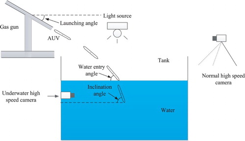
The complete experimental system is shown in Figure 1. The tank was 80 m in length and 30 m in width, with a water depth of 10 m. The launching angle of the gas gun could be adjusted according to requirements. The available stored maximum gas pressure was 0.8 MPa and the launching tube was 2.5 m long with an internal diameter of 205 mm. The vertical distance from the gun muzzle to water surface was 13 m. A normal high-speed camera with a resolution of 1280 × 800 and a shutter speed of 1000 fps was used to record the air flight path of the AUV. An underwater high-speed camera with a resolution of 1632 × 1200 and a shutter speed of 1000 fps was used to take photographs after the AUV entered the water, after which the data were transferred to a computer for processing. A three-axis accelerometer installed at the head of AUV was used to collect the changes in acceleration during water entry with a measuring range of 2000 g, a deviation of 1 g, and a sampling frequency of 60 kHz.

Figure 1. Schematic of the experimental system.

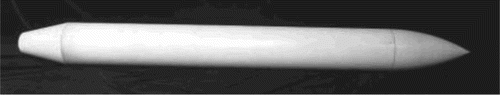
The mass of the AUV was 65.1 kg, with a volume of 0.052 m³, an average density of 1.252 kg/m³, and a rotational inertia 33.56 kg·m². The length of the AUV was 2 m, and gravity center was 1.08 m away from the tail (0.92 m away from the head). The concrete model dimensions and the physical object are shown in Figures 2 and 3, respectively.

Figure 2. Schematic of the AUV.

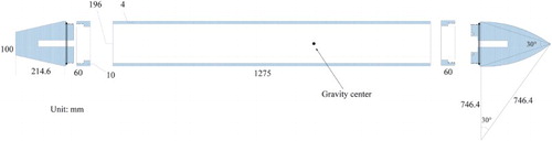
Figure 3. AUV physical map.

3. Data processing

3.1. Data processing of the normal high-speed camera images

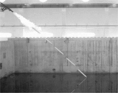
When the AUV is launched by a gas gun at a certain angle and speed (launching pressure), it flies in the air for a period of time and impacts the water surface to finish water entry. The motion state at the moment it enters the water cannot be directly obtained from the sensors but can be obtained from analyzing the air trajectory data. Figure 4 shows the motion trajectory of the AUV in the air with a launching pressure of 0.7 MPa and a launching angle of 45°. The sampling time is 0.05 s. The data were processed using the following steps.

Figure 4. AUV air trajectory.

First, the gravity center position and inclination angle were calculated. The gravity center of the AUV is 1.08 m away from its tail: (1) (2) where H_x and H_y are the coordinates of the head, and T_x and T_y are the coordinates of the tail.

Second, the initial state of the motion in the air was calculated. When the AUV flies through the air, its state is only related to gravity. The coordinate values of the gravity center and the change law of the inclination angle coincide with the flat parabolic and constant rotating speed motion: (3) (4) (5) where, X₀, v_x0, Y₀, v_y0, and ω_z can be calculated using a linear regression method.

Third, the motion state was calculated at the moment the AUV enters the water – that is, when T = t_in, the horizontal speed is V_{x_in} = v_x0, the vertical speed is V_{y_in} = v_y0 + gt₀ and the rotational angle speed is ω_in = ω_z. When the AUV enters water, the position and oblique angle of the model can be read directly from the images of the water entry.

Water entry impact experiments were conducted using different launching angles (15°, 25°, 30°, 35°, and 45°) with a set pressure (0.7 MPa), and using different launching pressures (0.6 MPa, 0.7 MPa, and 0.8 MPa) with a set launching angle (30°). The water entry states of the AUV under different launching conditions were calculated based on the above process, the results of which are shown in Tables 1 and 2.

Table 1. Motion state of the AUV entering the water with an initial launching angle of 30°.

Launching pressure (MPa)	0.60	0.70	0.80
Inclination angle (°)	63.54	59.93	52.76
Horizontal velocity (m/s)	19.86	21.70	24.13
Vertical velocity (m/s)	18.21	19.48	20.98
Rotational velocity (°/s)	33.17	25.43	16.76
Angle of attack (°)	−23.75	−18.02	−7.64
Axial velocity (m/s)	26.94	27.95	31.98

Table 2. Motion state of the AUV entering water the with an initial launching pressure of 0.7 MPa.

Launching angle (°)	15.00	25.00	30.00	35.00	45.00
Inclination angle (°)	64.06	60.72	59.93	49.54	49.12
Horizontal velocity (m/s)	29.24	21.86	21.70	21.51	22.21
Vertical velocity (m/s)	14.23	17.88	19.48	18.35	19.22
Rotational velocity (°/s)	28.54	26.16	25.43	18.68	6.84
Angle of attack (°)	−38.11	−11.44	−18.02	−9.07	−8.24
Axial velocity (m/s)	25.59	27.39	27.95	28.52	30.06

3.2. Data processing of the underwater high-speed camera images

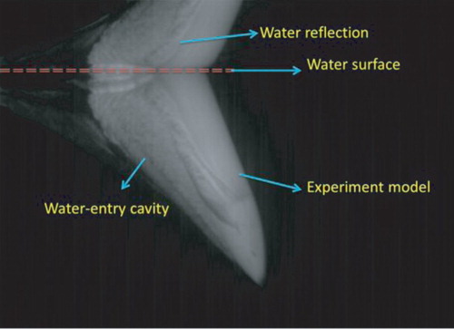
The normal high-speed camera captured the motion states of the AUV flying in the air, while the motion states after water entry were mainly captured by the underwater high-speed camera, which was fixed on a wall and could not move freely. Figure 5 shows the image that the camera captured 0.04 s after the AUV impacted on the water surface, in which the light area is the AUV and cavitation, and the dark area is the water.

Figure 5. Water entry process of the AUV captured by the underwater high-speed camera.

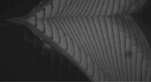
The AUV water entry with an initial launching angle of 30° and a launching pressure of 0.7 MPa is taken as an example to illustrate the data processing sequence. First of all, the camera data is sampled at a sampling frequency of 5 frames. Then, all the samples of the whole water entry process are drawn into the same field of view, and the approximate change in water entry attitude can be seen (Figure 6).

Figure 6. Water entry process in the same field of view (with a time interval of 0.005 s).

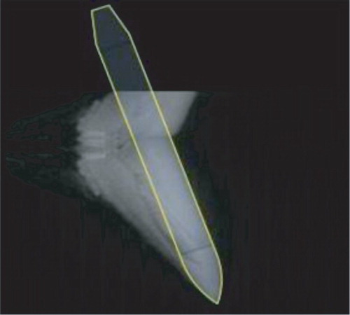
It can be seen that the inclination angle increases and the AUV is likely to turn over during the whole process of water entry. Due to the visual field limitations of the underwater camera, the head and the tail of the AUV cannot be seen in the same image. The images are completed to determine the attitude and the gravity center of the AUV at various moments (Figure 7). All the model outlines must be the same size in the view field so that the deviation caused by the differences of AUV outline when treated separately can be eliminated.

Figure 7. AUV outline selection.

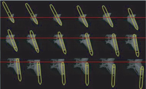
As shown in Figure 8, there is almost no cavitation in front of the AUV in each image where the outline is most distinct, which can be used to determine the inclination angle. By measuring the angle of the lines calibrated in Figure 8, the inclination angle is obtained in Table 3.

Figure 8. Inclination angle determination of the AUV.

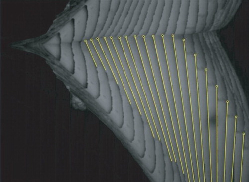
Table 3. Inclination angle changes of water entry.

Time (s)	0.020	0.025	0.030	0.035	0.040	0.045	0.050	0.055	0.060
Angle (°)	63.93	64.96	65.82	68.39	68.75	70.71	71.85	73.72	75.64
Time (s)	0.065	0.070	0.075	0.080	0.085	0.090	0.095	0.100	0.105
Angle (°)	77.57	79.59	81.71	83.72	85.78	87.18	89.75	92.44	93.74

The position and attitude of the AUV are determined based on its outline (Figure 7) and inclination angle (Table 3), and the location change of the gravity center in each image is obtained (Figures 9 and 10), in which the light line is the calibrated outline.

Figure 9. Position determination of the AUV.

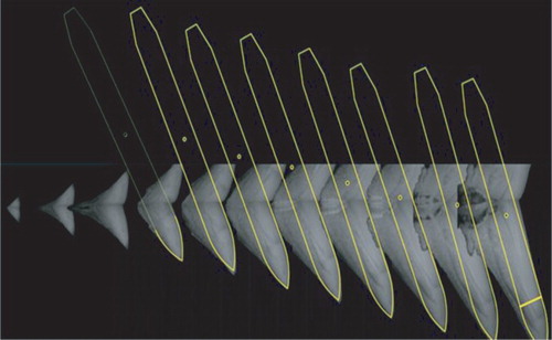
Figure 10. Position determination of the water entry process.

In Figure 9, the inclination angles in the first three images are not easy to measure due to its short water entry distance, which may cause errors in data processing. Therefore, the first three images are ignored. The absolute coordinate values of the gravity center with its origin at the bottom left corner of the image are obtained after data processing (Table 4).

Table 4. Coordinate values of the gravity center.

Time (s)	0.020	0.025	0.030	0.035	0.040	0.045	0.050	0.055	0.060
x-axis (mm)	1600.0	1493.9	1396.9	1272.2	1180.5	1075.3	983.9	891.6	801.6
y-axis (mm)	1531.1	1431.9	1341.4	1242.9	1125.1	1020.3	913.8	799.5	689.4
Time (s)	0.065	0.070	0.075	0.080	0.085	0.090	0.095	0.100	0.105
x-axis (mm)	732.1	651.4	588.9	522.3	458.6	394.1	347.7	299.5	247.3
y-axis (mm)	601.0	522.3	444.5	353.4	256.7	137.6	15.6	−111.0	−209.8

4. Numerical simulation of the water entry of an airborne-launched AUV

The commercial software CFX, which is a finite-volume program, was applied to simulate the water entry process of the airborne-launched AUV and the model used in simulation is the same size as the AUV used in above experiments.

4.1. Governing equations and turbulence model

The basic governing equations include continuity equations, momentum equations, Reynolds-averaged Navier–Stokes equations and energy conservation equations. As the conversion of energy is not related, the energy equations are not needed. The governing equations are expressed as follows: (6) (7) where is the ith component of the velocity vector, is the density of the fluid, is the pressure, and is the dynamic viscous coefficient.

The shear stress transport (SST) turbulence model is used in this study, which has proven to be highly successful in predicting complex fluid flows (Abrahama et al., 2014). The proper transport behavior can be obtained by a limiter to the formulation of the eddy-viscosity: (8) (9) where F₂ is a blending function that restricts the limiter to the wall boundary layer because the underlying assumptions are not correct for free shear flows, and S is an invariant measure of the strain rate.

4.2. Meshing of the computational domain

A prismatic mesh, which is obtained by stretching the non-structural plane along axial direction, was used in mesh generation. The number is 1.121.937 and the whole quality is over 0.6 (Figure 11). A circular region with a radius of 20 times the AUV length (40 m) was selected as the computational domain (Figure 12). Air and water were selected as the gas and liquid phases, respectively. The mesh near the AUV is locally refined to reduce calculation errors and increase the convergence speed (Figure 13). The time size is Δt = 5 × 10⁻⁵ s.

Figure 11. Mesh quality.

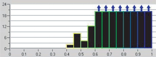
Figure 12. Computational domain.

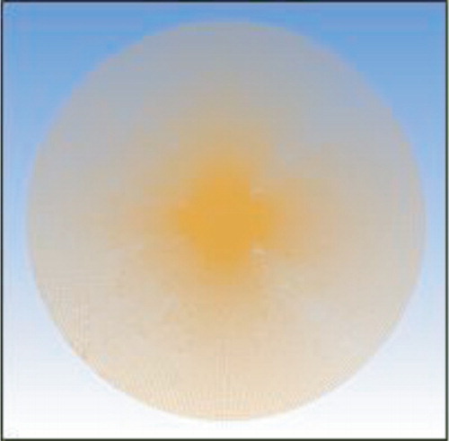
Figure 13. The mesh near the AUV.

4.3. Boundary conditions

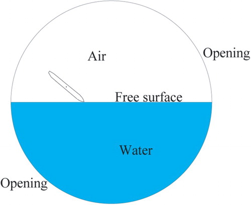
The boundary conditions of the computational domain are shown in Figure 14. ‘Opening’ was used to define the boundary type, which can be used for the outlet as well as the inlet. The ‘Step’ function (Equation (10)) was used to define the volume fraction of air and water for different coordinates. Dynamic grid technology was used to simulate the motion of the AUV, and the motion of the free surface was tracked using the volume of fluid (VOF) method. To improve the precision, a second-order backward Euler scheme was used. (10)

Figure 14. The boundary conditions.

4.4. Simulation conditions

In order to ensure enough initialization time and improve the accuracy, the top of the AUV is 4R away from the water surface along its axis, where R is the radius of the cylinder part in the middle of the AUV. A Dawning A840r-G system was used to conduct the simulations, with four OPTERON6176 (2.3 GHz), 12-core processors and 128 GB internal storage. As with the experiments, nine simulations were conducted with the values of initial velocity as shown in Tables 1 and 2. The total simulation time for all nine runs was 300 h. The properties of air and water are specified in Table 5.

Table 5. Properties of air and water.

Property	Air	Water
Density (kg/m^3)	1.19	997.00
Kinematic viscosity (m^2/s)	1.54e-5	8.93e-7
Dynamic viscosity (N s/m^2)	1.83e-5	8.9e-4

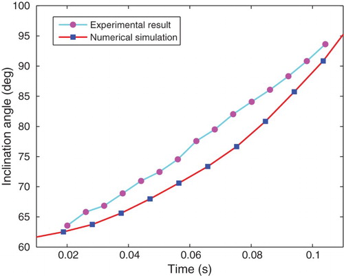
To keep the paper reasonably concise, only a comparison of the numerical and experimental results for the water entry process, the trajectory and the inclination angle are given for one of the nine runs in Figure 15 to 17, respectively, with an initial launching angle of 30° and a launching pressure of 0.7 MPa. The pressure contours during the water entry process are also given in Figure 15.

Figure 15. Water entry process and pressure contours in experiment and simulation where (a) t = 0.02 s, (b) t = 0.04 s, (c) t = 0.06 s, (d) t = 0.08 s, and (e) t = 0.10 s.

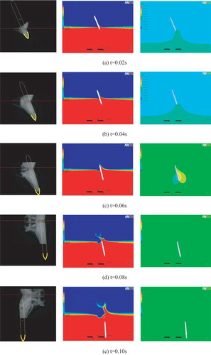
The simulation results depend on the initial conditions, mesh generation, turbulence model, etc., while the experimental data may be influenced by sensors, operation, environment and so on, so the results of the simulations and experiments not completely match, as shown in Figure 16 and 17. However, it can be seen that they coincide well with each other, and the simulation results can reflect spattering, angle deflection etc. in the experiments.

Figure 16. Comparison of the trajectory in the experimental and simulation results.

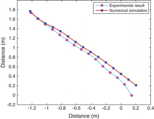
Figure 17. Comparison of the inclination angle in the experimental and simulation results.

5. Results analysis

5.1. Force loading of the water entry process

The initial water entry conditions are set, then the recorded overload of the accelerometer and the calculated overload of the simulation are compared. The initial launching pressure was 0.7 MPa, and a range of launching angles were used. The output forces in the numerical simulation were a series of discrete sequence points. The B-spline curve was applied in this paper in approximation and the corresponding results are shown in Figure 18.

Figure 18. Comparison of the experimental and simulation results at a pressure of 0.7 MPa for (a) θ = 10°, (b) θ = 15°, (c) θ = 20°, (d) θ = 25°, (e) θ = 30°, (f) θ = 35°, (g) θ = 40°, (h) θ = 45°, and (i) θ = 60°.

Note: X-ER = axial overload of experimental results; X-NS = axial overload of numerical simulation; Y-ER = radial overload of experimental results; Y-NS = radial overload of numerical simulation.

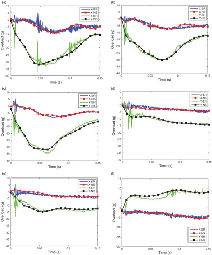
The results show that, in most cases, though the changes in the overload values calculated by the numerical simulation and the results obtained in the experiments are the same, there are certain differences mainly caused by neglected practical factors such as structure elastics and air cushion effects. The inconsistent directions of the radial overload in the experiments are caused by random collisions between the body and the inner wall of the gas gun when the AUV is launched. As the entry angle increases, the axial loads of the AUV also increase. Though vertical water entry experiments were not conducted due to impracticalities, it can be verified that the axial load is greatest when the AUV enters the water with vertical attitude. From the change of loads, the peak value of the axial impact load can be observed in a very short time after the head of the AUV enters the water and then the impact becomes stable after a rapid decrease. The radial impact load reduces with an increase in entry angle. If the AUV enters the water at a lower angle, the water entry impact of the radial direction and the bending moment should be taken into account. Moreover, the unstable water entry attitude caused by an extremely small angle should be noted, as it may lead to ricochet or flutter, even the body snap. As can be seen from the figures, both the water entry velocity and the entry angle have a great influence on the impact load of the water entry process.

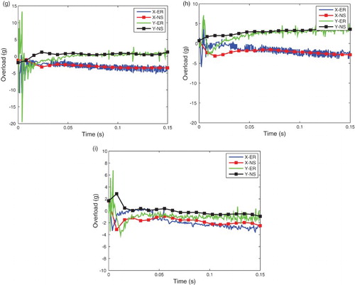
5.2. Changes in velocity

The changes in velocity with different launching angles under same pressure are shown in Figure 19. The velocity of the AUV reduces markedly in a short time. When the launching angle is 15°, 25°, 30°, 35°, and 45°, the velocity decreases by 6.97 m/s, 7.95 m/s, 8.48 m/s, 8.96 m/s, and 9.68 m/s, respectively. The velocities of AUV before and after water entry are shown in Table 6. The larger the water entry angle, the more the velocity of the AUV decreases, which coincides with the conclusion in Wei, Shi, and Wang (2012).

Figure 19. Change curves of water entry velocity.

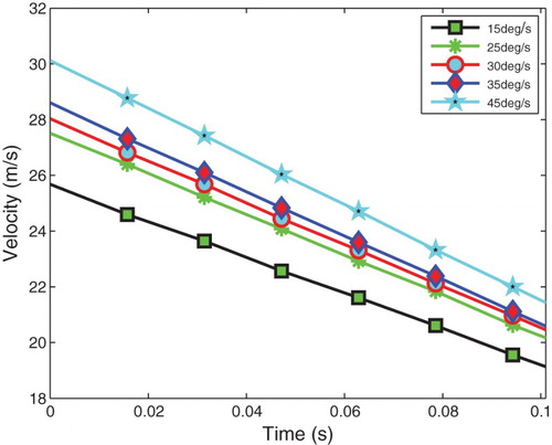
Table 6. Velocity changes of the AUV during water entry for different launching angles.

Launching angle (°)	15.00	25.00	30.00	35.00	45.00
Velocity before (m/s)	25.59	27.39	27.95	28.52	30.06
Velocity after (m/s)	18.62	19.44	19.47	19.56	20.38
Velocity change (m/s)	6.97	7.95	8.48	8.96	9.68

5.3. Cavitation in water entry

When an object enters water at high speed, the relatively large gradient change of pressure is observed at the edge of the body head. Cavitation occurs when the pressure is lower than that of saturated steam, with a negative effect on motion stability. The size and shape of cavitation cannot be directly read or measured, limited by experimental conditions in this paper, but its shape can be reflected by the pressure isosurface to some extent. The pressure isosurfaces of the simulations 30 ms after the AUV makes contact with the water surface with different launching angles under the pressure of 0.7 MPa are shown in Figure 20. It can be seen that the cavitation on its head becomes more obvious with the increase in launching angle when entry velocities are kept constant.

Figure 20. Cavitation shape of 30 ms after the AUV makes contact with the water surface at a pressure of 0.7 MPa for (a) θ = 15°, (b) θ = 25°, (c) θ = 30°, (d) θ = 35°, and (e) θ = 45°.

6. Conclusion

In this paper, the water entry process of a full-size AUV launched using a gas gun was investigated under varying conditions to obtain a series of accurate load data. The water entry process of the AUV was simulated by the commercial software package CFX and the accompanied phenomena such as cavitation were observed. The simulation and experimental results are in good agreement. The analysis shows that the impact load reaches its peak value in a very short time at the initial water entry of the AUV and then gradually reduces and stabilizes. As the water entry angle increases, the axial load increases and the radial load decreases. Vertical water entry should be avoided and the velocity should be reduced as much as possible to avoid damage to the sophisticated components in the head of the AUV. This paper also examined the relationship between the launching angle and cavitation at the AUV’s head with a constant velocity.

Several factors should be taken into consideration when launching an AUV from an aircraft, including structure strength, entry site accuracy, trajectory and attitude underwater. Limited by the experimental conditions, the paper obtains preliminarily water entry impact load data for launching a full-size AUV from the air into the water, which can provide reference information for AUV structural design decisions and launch condition selection. In future studies, improvements will be made to the experimental and numerical simulation conditions, and the influence of different AUV masses and head shapes on the water entry impact and cavitation on the motion states will be explored.

Disclosure statement

No potential conflict of interest was reported by the authors.

Additional information

Funding

This work was supported by the National Natural Science Foundation of China: [grant number 61472443].

References

- Abrahama, J., Gorman, J., Reseghetti, F., Sparrowa, E., Stark, J., & Shepard, T. (2014). Modeling and numerical simulation of the forces acting on a sphere during early-water entry. Ocean Engineering, 76, 1–9. doi:1016/j.oceaneng.2013.11.015 doi: 10.1016/j.oceaneng.2013.11.015
- Aristoff, J. M., Truscott, T. T., Techet, A. H., & Bush, J. W. M. (2010). The water entry of decelerating spheres. Physics of Fluids, 22, 032102. doi:doi:10.1063/1.3309454
- Benson, H. E. (1966). Water impact of the Apollo spacecraft. Journal of Spacecraft and Rockets, 3, 1282–1284. doi:doi:10.2514/3.28640
- Burt, F. S. (1961). Hydrodynamic research. British Journal of Applied Physics, 12, 323–328. doi:10.1088/0508-3443/12/7/303 doi: 10.1088/0508-3443/12/7/303
- Epely-Chauvin, G., De Cesare, G., & Schwindt, S. (2014). Numerical modeling of plunge pool score evolution in non-cohesive sediments. Engineering Applications of Computational Fluid Mechanics, 8, 477–487. doi:10.1080/19942060.2014.11083301 doi: 10.1080/19942060.2014.11083301
- Eroshin, V. A., Romanenkov, N. I., & Serebryakov I. V. (1980). Hydrodynamic forces produced when blunt bodies strike the surface of a compressible fluid. Akademiia Nauk Sssr Izvestiia Mekhanika Zhidkosti I Gaza, 15, 829–835. doi:doi:10.1007/BF01096631
- Gu, J. N., Zhang, Z. H., & Fan, W. J. (2005). Experimental study on the penetration law for a rotating pellet entering water. Explosion and Shock Waves, 25, 341–349. Retrieved from http://www.bzycj.cn/CN/volumn/home.shtml
- Guo, Z. T., Zhang, W., Xiao, X. K., Wei, G., & Ren, P. (2012). An investigation into horizontal water entry behaviors of projectiles with different nose shapes. International Journal of Impact Engineering, 49, 43–60. doi:10.1016/j.ijimpeng.2012.04.004 doi: 10.1016/j.ijimpeng.2012.04.004
- Kleefsman, K. M. T., Fekken, G., Veldman, A. E. P., Iwanowski, B., & Buchner, B. (2005). A volume-of-fluid based simulation method for wave impact problems. Journal of Computational Physics, 206, 363–393. Retrieved from http://www.journals.elsevier.com/journal-of-computational-physics/ doi: 10.1016/j.jcp.2004.12.007
- Li, Q., Shi, X. H., & Cao, Y. P. (2009). Numerical simulation of the influence of torpedo head shape to water entry. Journal of Projectiles;Rockets;Missiles and Guidance, 29, 167–170. doi:doi:10.15892/j.cnki.djzdxb.2009.04.037
- Ma, Q. P., He, C. T., Wang, C., Wei, Y. J., Lu, Z. L., & Sun, J. (2014). Experimental investigation on vertical water-entry cavity of sphere. Explosion and Shock Waves, 34, 174–180. Retrieved from http://www.bzycj.cn/CN/volumn/home.shtml
- Panciroli, R., Abrate, S., Minak, G., & Zucchelli, B. (2012). Hydroelasticity in water-entry problems: Comparison between experimental and SPH results. Composite Structures, 94, 532–539. doi:doi:10.1016/j.compstruct.2011.08.016
- Pan, C. J., & Guo, Y. C. (2013). High altitude air-launched AUV’s complete trajectory simulation system based on simulink. Computer Engineering and Applications, 49, 222–226. doi:doi:10.3778/j.issn.1002-8331.1210-0229
- Park, M. S., Jung, Y. R, & Park, W. J. (2003). Numerical study of impact force and ricochet behavior of high speed water-entry bodies. Computers&Fluids, 32, 939–951. doi:doi:10.1016/S0045-7930(02)00087-7
- Shams, A., Jalalisendi, M., & Porfiri, M. (2015). Experiments on the water entry of asymmetric wedges using particle image velocimetry. Physics of Fluids, 27, 027103-1–027103-26. doi:doi:10.1063/1.4907745
- Von Karman, T. (1929). The impact of seaplane floats during landing. Washington, DC: National Advisory Committee for Aeronautics.
- Wagner, V. H. (1932). Phenomena associated with impacts and sliding on liquid surfaces. Journal of Applied Mathematics and Mechanics, 12, 193–215. doi:10.1002/zamm.19320120402.
- Wang, S., Su, Y.M., Wang, Z.L., Zhu, X.G., & Liu, H. X. (2014). Numerical and experimental analyses of transverse static stability loss of planning craft sailing at high forward speed. Engineering Applications of Computational Fluid Mechanics, 8, 44–54. doi:10.1080/19942060.2014.11015496 doi: 10.1080/19942060.2014.11015496
- Wang, Y. H. (2008). Analysis and related technology research on water enter impact response of air-drop torpedo (Unpublished doctoral dissertation). Northwestern Polytechnical University, Xian.
- Wei, Z. Y., Shi, X. H., & Wang, Y. H. (2012). The oblique water entry impact of a torpedo and Its ballistic trajectory simulation. International Journal of Numerical Analysis and Modeling, 9, 312–325. Retrieved from http://www.math.ualberta.ca/ijnam/
- Yang, Q. Y., & Qiu, W. (2012). Numerical simulation of water impact for 2D and 3D bodies. Ocean Engineering, 43, 82–89. doi:doi:10.1016/j.oceaneng.2012.01.008
- Zhang, K., Yan, K., Chu X. S., & Chen, G. Y. (2010). Numerical simulation of the water-entry of body based on the lattice Boltzmann method. Journal of Hydrodynamics, Ser. B, 22, 872–876. doi:doi:10.1016/S1001-6058(10)60044-3
- Zhang, X. H., Du, M. L., & Ma, C. S. (2010). Water impact simulations and analyses of space capsule response characteristics. Journal of Tsinghua University, Science and Technology, 50, 1297–1301. Retrieved from http://jst.tsinghuajournals.com/CN/1000-0054/home.shtml