
ABSTRACT
The unsteady phenomenon abounds in centrifugal compressors and significantly affects the compressor performance. In this paper, unsteady simulations are carried out to investigate the aerodynamic performance of a process-unshrouded centrifugal compressor and the unsteady mechanism in the vaned diffuser. The predicted stage performance and pressure fluctuations at some locations are in good agreement with experimental data. The predicted main pressure fluctuation frequency spectrums at the diffuser inlet and outlet are consistent with the measured results. The results indicate that at the inlet of the diffuser there are two pressure peaks in a passage cycle. The higher pressure peak relates to the impeller wake and the lower peak is connected with the vortex generated at the diffuser’s leading edge. With a decrease in the mass flow coefficient, the vortex core region becomes larger and the lower pressure peak becomes more pronounced. The change in circumferential flow angle at the diffuser inlet is mainly responsible for the unsteadiness in the diffuser flow field, which in turn affects the inlet incidence of the diffuser vane and the vane loading distributions.
Nomenclature
| Cp | = | Heat capacity 1008.42 (J/kg/K) |
| Cps | = | Static pressure recovery coefficient |
| Cpt | = | Total pressure loss coefficient |
| D2 | = | Impeller outlet diameter (m) |
| D3 | = | Diffuser inlet diameter (m) |
| D4 | = | Diffuser outlet diameter (m) |
| k | = | Adiabatic exponent |
| n | = | Rotational speed (rev/min) |
| Ps | = | Pressure (Pa) |
| PsN | = | |
| Pt | = | Total pressure (Pa) |
| PtN | = | |
| Qm | = | Mass flow rate (kg/s) |
| R | = | Radius |
| R2 | = | Impeller outlet radius (m) |
| R | = | Ideal gas constant R = 287 (J/kg/K) |
| Mu2 | = | Machine Mach number |
| T | = | The time it takes an impeller blade to pass one impeller passage |
| Tt | = | Total temperature (K) |
| U2 | = | Circumferential velocity at the impeller outlet |
| VC | = | Circumferential velocity in the absolute coordinate system |
| VR | = | Radial velocity in the absolute coordinate system |
| η | = | Polytropic efficiency |
| = | Stagnation density (kg/m3) | |
| τ | = | Head coefficient |
| ϕ1 | = | Flow coefficient |
Subscripts and superscripts
| d | = | Diffuser |
| in | = | Inlet |
| out | = | Outlet |
1. Introduction
Centrifugal compressors are widely used in many industries, such as aviation, refrigeration, fertilizers, oil and gas, etc. The efficiency (η) is one of the primary performance parameters for centrifugal compressors. Due to some inevitable aerodynamic losses resulting from the secondary flow, leakage flow and impeller–diffuser interactions (IDIs), the maximum theoretical efficiency is 90 to 92% (Sorokes, Kuzdzal, & Zhang, Citation2011). For a medium flow coefficient centrifugal compressor, the efficiency has been increased from70 to 75% in the 1950s to about 90% in the 2010s. Nowadays, due to the increase in energy consumption and global warming, attaining an even higher efficiency has attracted much attention. As well as the loss in the impeller, the loss in the diffuser also constitutes a large portion of the total loss in the centrifugal compressor. Therefore, understanding the loss mechanism in a diffuser is significant for the improving the performance in a compressor.
The diffuser is designed to transform the high kinetic energy of the fluid coming from the impeller into the pressure energy. It is also intended to provide a more uniform flow field for the subsequent components. The performance of the diffuser depends on the impeller exit flow field. Conversely the diffuser also has an influence on the performance of the impeller. This is the so-called ‘impeller–diffuser interaction’ (IDI). Y. W. Liu, Liu, and Lu (Citation2010) analyzed the transonic centrifugal compressor stage and found that the impeller flow field after the 70% chord length is influenced by the IDI. The IDI generates a 2% fluctuation for the total pressure ratio and a 13° variation for the impeller outlet flow angle.
The IDI is complex and has been studied for different centrifugal compressors. Kai, Heinz, and Reinhard (Citation2003a, Citation2003b) and Robinson, Casey, Hutchinson, and Steed (Citation2012) studied the impact of the size of the gap between the impeller and the vaned diffuser on the performance of the vaned diffuser; their findings indicate that a smaller gap results in a higher efficiency and a stronger IDI effect. Wilkosz, Zimmermann, Schwarz, Jeschke, and Smythe (Citation2014) and Anish, Sitaram, and Kim (Citation2014) investigated the impact of the IDI on the centrifugal compressors with both high and low Mach numbers, finding that the IDI strongly affects the aerodynamic performance of the diffuser and that it must be considered in the detailed design process. Anish et al. (Citation2014) noted that the main factor influencing the diffuser instability is the circumferential variation of the flow angle at the leading edge of the diffuser vane. The aerodynamic loss in the diffuser is induced mainly by the generation and shedding of the vortexes which exist on the diffuser vane leading edge, on the suction side of the diffuser vane near the hub and on the diffuser vane trailing edge. Fujisawa, Hara, and Ohta (Citation2016) applied the oil-film method and computational fluid dynamics (CFD) analysis to the investigation of the leading-edge vortex structure on the leading edge of a wedge diffuser and the rotating stall in a centrifugal compressor. They pointed out that the diffuser stall might be caused by the evolution of the leading-edge vortex. The authors designed a hub-side tapered diffuser vane. The experimental and CFD results show that the tapered diffuser vane can suppress the evolution of the leading-edge vortex and consequently control the diffuser stall inception during the off-design operation. L. J. Liu, Xu, and Zhang (Citation2002) found that there is a low-speed stagnation region near the leading edge of the diffuser vane which makes the circumferential distribution of the velocity field more nonuniform in front of the diffuser vane. The wake loss increases and the flow becomes unstable in the whole diffuser passage. Gallier, Lawless, and Fleeter (Citation2010) found that there is a highly nonuniform flow field in the vaneless space between the impeller and the diffuser that results in a large variation in the flow angle at the diffuser vane leading edge and subsequently causes an unsteady vane loading. Vogel, Abhari, and Zemp (Citation2014) indicated that with an increase in the flow coefficient, the pressure fluctuation amplitude decreases in the diffuser passage. Zhao et al. (Citation2015) employed CFD techniques to analyze the interaction of the inlet guide vane and the impeller, observing two loading peaks at the impeller blade leading edge for a small mass flow coefficient during a passage cycle.
Although the IDI has been extensively studied, the flow fields in both the impeller and the diffuser are not completely understood, since different designs have various flow structures. There are a lot of diffuser types, such as vanless diffusers, 2D vaned diffusers, 3D vaned diffusers (Strohmeyer & Hildebrandt, Citation2012), tandem diffusers (Zhou, Wang, & Liu, Citation2014), and so on. This paper focuses on a radial 2D-vaned diffuser in an unshrouded centrifugal compressor and is devoted to analyzing the IDI and unsteadiness.
2. Test facilities
The measurements were performed on the centrifugal compressor test rig at the Shenyang Blower Works Group Corporation. displays the test section of the centrifugal compressor test facility. There are four total pressure probes (1) and four thermocouple probes (2) mounted at the inlet of the compressor at different heights. At the outlet of the compressor there are one comb probe (3) and four thermocouple probes (2) also at different heights (as shown in , the five probes can be rotated by using the rotary knob (5)). The orifice flowmeter (4) is mounted at the inlet of the compressor, which is far from the test probes. These probes are shown in . The total pressure is measured by Rosemount 3051CD pressure transmitters which have a 0.075% accuracy, and the thermocouple probe is B-type. During the experiment, the probes at the outlet were rotated and positioned at 20 circumference positions in a 40° range tgat covers two return vane passages. The signal sampling card collected 4000 data in 10 seconds after the signals were stable, then the area-averaged and time-averaged total pressure and total temperature were obtained.
Figure 1. Centrifugal compressor test facility (test section).
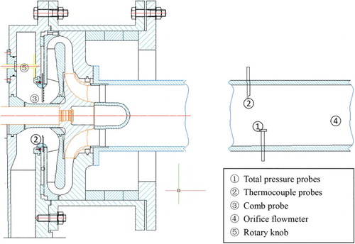
Figure 2. Measuring positions at the outlet of the return channel.
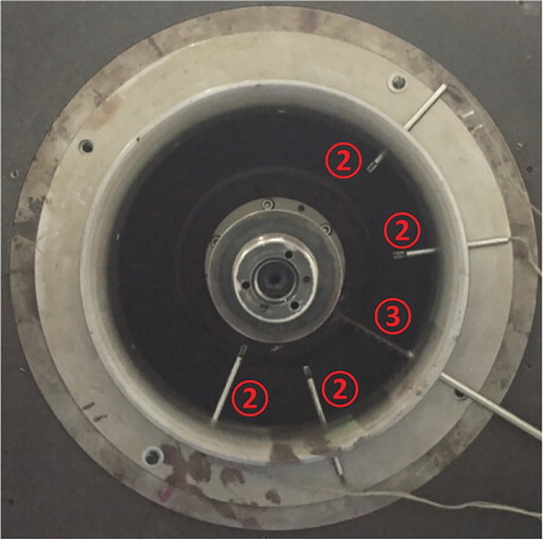
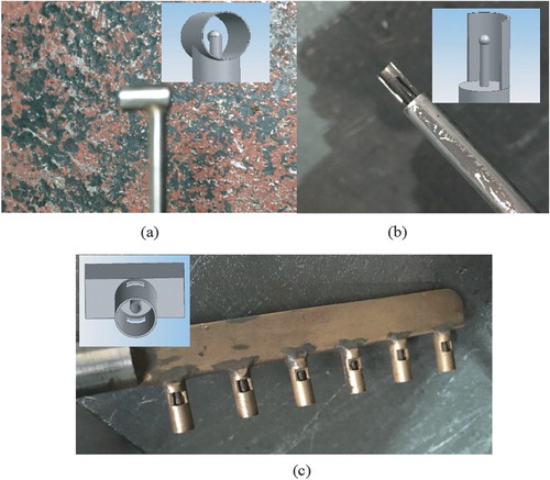
Figure 3. Test probes: (a) total pressure probe, (b) thermocouple probe, and (c) comb probe.
3. Numerical methods
3.1. Numerical scheme
ANSYS CFX v14.0 was utilized to simulate the flow field in the centrifugal compressor. The single passage unsteady calculation method of ‘profile transformation’ (ANSYS, Citation2011a) was employed to analyze the IDIs for unsteady simulations. According to the profile transformation method, the flow interaction across the rotor–stator interfaces is handled by the pitch scaling mechanism. The time step was taken to be the time of an impeller blade passing 1/360 of a circle. This value is the optimum time step according to Anish and Sitaram (Citation2009) and Anish et al. (Citation2014). The ‘stage’ method (ANSYS, Citation2011a) was adopted for analyzing the IDIs for steady simulations. The stage model performs a circumferential averaging of the fluxes through bands on the interface. The stage averaging at the interface incurs a one-time mixing loss which accounts for time-averaged interaction effects. The Shear Stress Transport (SST) turbulence model of Menter (Citation1994) was employed because of its success in modeling flows in an adverse pressure gradient, and Mangani, Casartelli, and Mauri (Citation2012) have proved that this turbulence model is suitable for centrifugal compressor calculations. A ‘high resolution’ advection scheme (ANSYS, Citation2011a) was employed for all equations except for the turbulence equation, which uses a first-order upwind scheme.
3.2. Computational domains
A single-flow passage domain with periodic boundary conditions was employed to simulate the flow field of the unshrouded centrifugal compressor. The compressor is composed of the guide vane, the unshrouded backswept impeller, the vaned diffuser and the return channel. The main dimensions of the centrifugal compressor are listed in . The guide vane is kept in the same position where there is a 60° angle between the chord of the vane and the circumferential direction. Note that all angles in this paper refer to the angle between the flow direction and the circumferential direction.
Table 1. Primary geometric information of the centrifugal compressor.
shows a sketch of the meridional channel, and sections 0 to 4 represent the inlet of the whole domain, the inlet of the impeller, the impeller exit, the diffuser outlet and the return channel exit, respectively. An unstructured tetrahedral grid generated by the Integrated Computer Engineering and Manufacturing code for Computation Fluid Dynamics (ICEM CFD) software (ANSYS, Citation2011b) was applied to the inlet domain (section 0-0 to section 1-1), while a structured mesh generated by Autogrid (NUMECA, Citation2009) was used for the other domains. lists the number of grid nodes for each part after a grid-independence study. The meshes of the impeller passage and the diffuser passage are shown in . The average Y+ value is almost 3 for the first nodes away from the walls in the simulations.
Figure 4. Sketch of the meridional channel.
Figure 5. Grid maps for (a) the impeller and (b) the diffuser.
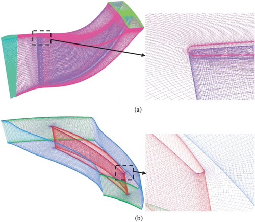
Table 2. Domain grid node numbers.
3.3. Boundary conditions
The measured total pressure, total temperature and inlet flow angles were specified at the inlet. The mass flow rate in the experiments was imposed at the outlet. The periodic conditions were imposed for the pitch-wise boundaries. For steady calculations, the steady-state ‘stage interface’ method (ANSYS, Citation2011a) was employed for interfaces between blade rows, which uses a mixing-plane interface approach. For unsteady calculations, the ‘transient rotor stator’ method (ANSYS, Citation2011a) was used. The machine Mach number Mu2 = 0.75 and U2 = 244.3 m/s. Three different mass flow rates were considered in the present work: ϕ1 = 0.118 for Case 1 (108.3% of the design mass flow coefficient), ϕ1 = 0.109 for Case 2 (100% of the design mass flow coefficient), and ϕ1 = 0.101 for Case 3 (92.7% of the design mass flow coefficient).
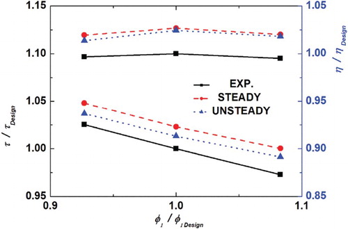
Figure 6. Comparison of the steady and unsteady results with the experimental data.
4. Results and discussion
4.1. Analysis of the centrifugal compressor performance
compares the predicted normalized polytropic efficiency and normalized head coefficient with the experimental data for three different flow coefficients. Time-averaged results were used for the unsteady simulations. Both steady and unsteady simulations over-predict these two parameters, but the changing trends of these parameters with ϕ1 are consistent with measurements (time-averaged results are used for comparison for the unsteady simulations). The results of the unsteady runs are closer to the experimental data, especially for the head coefficient. displays the predicted relative errors; it can be seen that the relative errors of the unsteady results are lower than those of the steady results, but all errors are below 3%. This demonstrates that the predicted results are sufficiently reliable.
Table 3. Relative errors of efficiency and head coefficient.
Due to the use of the mixing-plane method in steady simulations, the flow field after the interface between the impeller and the diffuser becomes more uniform than the actual situation. The mixing-plane method neglects transient interaction effects which cause a 3% increase in the total pressure (PtN) for steady simulations compared to the average value of PtN for unsteady calculations at the entrance of the diffuser. Meanwhile, the total temperature in steady simulations is also higher, which is the main reason for the differences between the unsteady and steady results.
Figure 7. Frequency spectrum of the pressure fluctuations at the inlet of the diffuser.
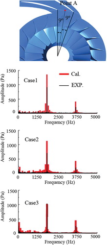
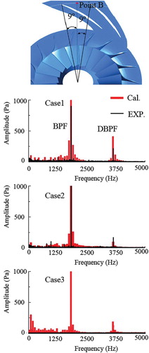
Figure 8. Frequency spectrum of the pressure fluctuations at the outlet of the diffuser.
4.2. Analysis of the pressure fluctuations in one diffuser passage
To understand the loss mechanism in the diffuser, pressure parameters at the diffuser inlet and outlet are examined. Point A is located at the shroud of the diffuser entrance and is in the middle of two diffuser vane leading edges (), while Point B is located at the shroud of the diffuser exit and is also in the middle of two diffuser vanes (). presents fast Fourier transformation (FFT) results of the predicted and measured pressure fluctuations at Point A, and presents the results for Point B. In the measurements, the sampling frequency is 10,240 Hz and with 52,000 sampling points; thus, the frequency resolution is 0.2 Hz. Li, Zhang, and Zhang (Citation2014) described the measuring system in detail. In the unsteady calculations, the sampling frequency is 34,658 Hz but there are only 400 sampling points (considering the time-cost of the calculations), therefore the frequency resolution is 86.4 Hz in the calculations. It can be seen from Figures and that the predicted blade passing frequency (BPF) and double blade passing frequency (DBPF) are in good agreement with the experimental data. However, the predicted amplitude is higher than the measured values. Through the spectrum analysis for Point A, it was found that the measured amplitudes of the BPF and DBPF for Case 2 are smaller than those of Case 1 and Case 3. This is understandable, as compared to Case 2, which uses the design mass flow rate, the incidence angle gets smaller for Case 1 with the large mass flow rate at the diffuser inlet and larger for Case 3 with the small mass flow rate at the diffuser inlet. Unsteadiness for Case 1 and Case 3 theoretically becomes stronger than that of Case 2; therefore the pressure fluctuations are larger for Case 1 and Case 3 than for Case 2, as presented in the measurements at Point A. However the predicted amplitudes of the BPF and DBPF slightly decrease as the flow coefficient decreases, which is caused by numerical errors. In contrast to Point A, the predicted and measured amplitudes of the primary frequencies at Point B are similar for Case 1 and Case 2. It should be mentioned that the measured data for Case 3 are omitted in due to the ridiculous results. The amplitudes of the BPF and DBPF at Point B are smaller than at Point A due to the flow diffusion and mixing effect in the diffuser flow passage.
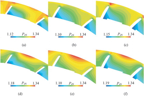
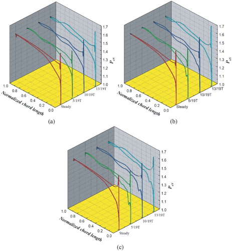
The changing trend of the pressure fluctuations with the time at Points A and B is shown in for Case 1, Case 2 and Case 3. It can be seen that PsN increases as the mass flow rate decreases, while the pressure at the diffuser inlet changes with time. The maximum pressure occurs at 5/19T, 6/19T and 7/19T at Point A for Case 3, Case 2 and Case 1, respectively. These times correspond to the locations where an impeller blade is close to the suction side of the diffuser vane. With an increase in the mass flow rate, the position of the impeller blade corresponding to the maximum pressure moves to the middle of the diffuser passage. This is ascribed to the high PsN zone being closer to the pressure side of the impeller blade for a large mass flow rate, while it is located between the impeller blade suction side and the impeller blade pressure side for a small mass flow rate (). Moreover, this phenomenon exists at all span locations for Case 1 and Case 3. This implies that the flow angle decreases with the mass flow rate and the pressure gradient direction is turned to the radial direction.
Figure 9. Pressure fluctuations with time for (a) Point A and (b) Point B.
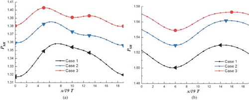
Figure 10. Distributions of PsN at 0/19T: (a) 95% span for Case 1, (b) 50% span for Case 1, (c) 5% span for Case 1, (d) 95% span for Case 3, (e) 50% span for Case 3, and (f) 5% span for Case 3.
Due to the diffusion and mixing effect in the diffuser flow passage, PsN at Point B is higher than it is at Point A, and the pressure fluctuation of PsN at Point B is smaller than it is at Point A.
4.3. Impeller–diffuser interactions (IDIs)
shows the entropy distributions on the plane at 95% span of the impeller and the diffuser for Case 1 and Case 3. It can be observed that the entropy for Case 3 is generally greater than that of Case 1. For Case 3, there are two high-entropy regions – the impeller wake region (referring to the low flow angle zones at the impeller exit) and the leading-edge region of the diffuser (). Higher entropy implies higher loss in these regions. At the time of 0/19T, the impeller wake propagates into the diffuser leading edge and the region close to the suction side of the diffuser vane occupies larger entropy values. At 5/19T, the high-entropy region is enlarged. At 10/19T, the high-entropy region moves from the suction side to the flow passage. At 13/19T, the next impeller wake is reaching the diffuser leading edge. In Case 1 there is a smaller area with large entropy than there is in Case 3 in the vicinity of the diffuser leading edge, and it is more evident that regions with high and low entropy alternately move to the diffuser passage.
Figure 11. Entropy distribution at 95% span for Case 1 and Case 3.
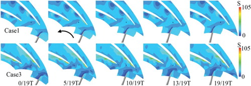
Figure 12. Distributions of flow angles at 95% span for Case 1 and Case 3.
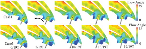
Figure 13. Distributions of streamline at 95% span at 13/19T for: (a) Case 1 and (b) Case 3.
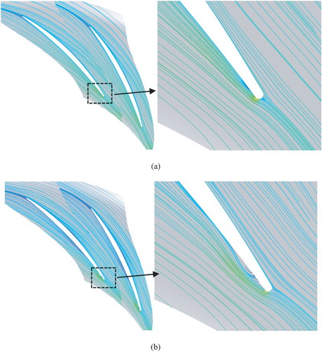
Figure 14. Vortex core regions within the diffuser passage for: (a) Case 1, (b) Case 2, and (c) Case 3.
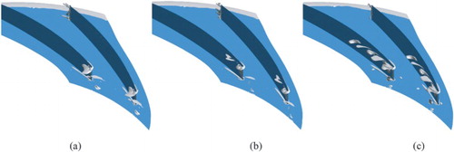
Figure 15. Case 3 at 95% span of diffuser inlet (R/R2 = 1.04): (a) pressure distribution and (b) flow angle distributions.
As shown in , the fluid with high entropy generated by the diffuser leading edge passes Point A at 13/19T. This is related to the second high-pressure value in . At Point A there are two peak pressure values in a passage cycle; one corresponds to the impeller wake and the other is associated with the large-entropy region generated at the diffuser leading edge.
Figure 16. (a) total pressure loss coefficient Cpt of diffuser and (b) static pressure recovery coefficient Cps of diffuser.
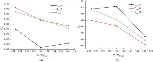
Figure 17. Loading distributions of the diffuser vane for Case 3 at: (a) 10% span, (b) 50% span, and (c) 90% span.
presents the distributions of the flow angles at 95% span of the impeller and the diffuser for Case 1 and Case 3. It can be seen that there are two recirculation regions (where the flow angle is lower than zero) on this plane for both Case 1 and Case 3. One region is located at the impeller outlet, which is called the impeller outlet recirculation region, and the other is located in the leading-edge region of the diffuser vane, which is called the diffuser leading-edge recirculation region. The impeller outlet recirculation region is mainly caused by the impeller wake, while the diffuser leading-edge recirculation region is a consequence of the high angle of attack at the diffuser leading edge. By analysis, it is obtained from the unsteady results in that the area of the impeller outlet recirculation region is obviously enlarged at 10/19T. In addition, at 13/19T when the impeller outlet recirculation region approaches the diffuser leading edge, the two recirculation regions overlap. This phenomenon is more distinct for Case 3, implying that the IDI has a larger influence on the two recirculation regions for a small flow coefficient.
4.4. Physical explanation of the diffuser vane leading-edge vortex
depicts the distributions of the streamlines at 95% span of the diffuser passage for Case 1 and Case 3 at 13/19T. There is a small recirculation region near the leading edge for both Case 1 and Case 3, the area of which is larger in Case 3 than in Case 1. The recirculation region represents a high-loss area that is responsible for an increase in the entropy at the leading edge of the vane ().
shows the vortex core regions (the isosurface of the swirling strength) near the leading edge of the diffuser vane for the three cases. This vortex is also observed by Anish et al. (Citation2014). As the mass flow coefficient decreases, the area of the vortex core region increases – that is to say, the strength of the vortex is enhanced. Through comparisons with Figures , and , it is concluded that the second high-pressure value in is related to this leading-edge vortex. Since the vortex core region is extended as the mass flow coefficient decreases, the second pressure peak gradually becomes more apparent ().
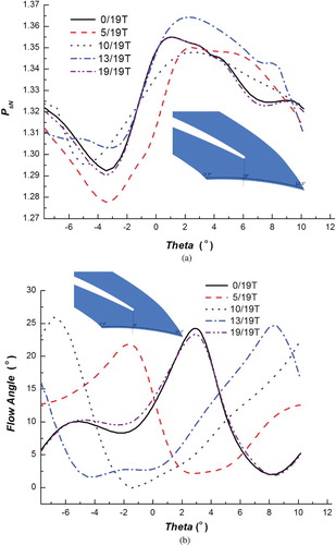
To further interpret the mechanism of the leading-edge vortex of the diffuser vane, displays the distributions of the pressure and the flow angle at 95% span of the diffuser inlet (R/R2 = 1.04) for Case 3. Locations with high or low pressure change marginally with time but the large flow angle location alters significantly with the time. These denote that the unsteadiness in the diffuser flow fields is greatly attributed to the unsteadiness of the circumferential flow angle at the inlet. The latter causes the periodic variation in the angle of attack at the diffuser vane leading edge. This incidence variation leads to the generation and shedding of the diffuser vane leading-edge vortex.
4.5. Analysis of diffuser performance
compares the total pressure loss coefficients (Cpt) and static pressure recovery coefficients (Cps) of the diffuser for the three cases with different flow coefficients (see the note in for details). It can be seen from that Cpt_A is lower than Cpt_B and Cpt_C, while Cps_A is higher than Cps_B and Cps_C. This is due to a relatively uniform diffuser inlet flow field produced by the mixing-plane method used in the steady calculations. The Cpt and Cps of B are similar to those of C.
presents the distributions of the vane loading (PsN) at different spans in a diffuser vane gained from steady and unsteady calculations for Case 3. The loading curves obtained from steady calculations change smoothly along the chord-wise direction, while the unsteady loading curves have noticeable fluctuations. The pressure at the suction side is higher than the pressure at the pressure side after about 50% chord length for the unsteady results. This phenomenon is continuous in the unsteady results, due to the lack of artificial mixing of the jet-wake flow field after the impeller is considered in the unsteady mode. This unsteady inlet flow condition is responsible for the diffuser vane loading fluctuation. As can be seen from , the unsteady inlet flow condition mainly lies in the unsteadiness of the circumferential flow angle.
5. Conclusions
Steady and unsteady calculations have been carried out to simulate the flow fields inside a process unshrouded centrifugal compressor with a vaned diffuser. The numerical results obtained from both the steady and unsteady simulations are in good agreement with the experimental data in terms of the stage efficiency and head coefficient around the design point. The predicted main pressure fluctuation frequency spectrums (the BPF and DBPF) at the inlet and outlet of the diffuser obtained from the unsteady calculations are consistent with the measured values. There are two pressure peaks in a passage cycle at the diffuser inlet. Predicted flow fields indicate that the higher-pressure peak is related to the impeller wake and that the lower-pressure peak is induced by the vortex generated at the diffuser leading edge. The generation and shedding of this leading-edge vortex is closely related to the altering inlet flow angle in the circumferential direction.
The above conclusions are derived from the calculation for a single passage of a centrifugal compressor stage with a middle flow coefficient. To improve the feasibility of these findings, whole passage calculations need to be performed in the future.
Acknowledgments
The authors gratefully acknowledge the support of Shenyang Blower Works Group Corporation for providing the geometric parameters and experimental results of the centrifugal compressor studied in the paper.
Disclosure statement
No potential conflict of interest was reported by the authors.
References
- Anish, S., & Sitaram N. (2009). Computational investigation of impeller–diffuser interaction in a centrifugal compressor with different types of diffusers. Proceedings of the Institution of Mechanical Engineers, Part A: Journal of Power and Energy, 223, 167–178. doi: 10.1243/09544089JPME239
- Anish, S., Sitaram, N., & Kim, H. D. (2014). A numerical study of the unsteady interaction effects on diffuser performance in a centrifugal compressor. Journal of Turbomachinery, 136, 011012. doi: 10.1115/1.4023471
- ANSYS. (2011a). ANSYS CFX version 14.0. Retrieved from http://www.ansys.com/
- ANSYS. (2011b). ANSYS ICEM CFD version 14.0. Retrieved from http://www.ansys.com/
- Fujisawa, N., Hara, S., & Ohta, Y. (2016). Unsteady behavior of leading-edge vortex and diffuser stall in a centrifugal compressor with vaned diffuser. Journal of Thermal Science, 25(1), 13–21. doi: 10.1007/s11630-016-0829-z
- Gallier, K., Lawless, P. B., & Fleeter, S. (2010). Particle image velocimetry characterization of high-speed centrifugal compressor impeller–diffuser interaction. Journal of Propulsion and Power, 26(4), 784–789. doi: 10.2514/1.38663
- Kai, U. Z., Heinz, E. G., & Reinhard, N. (2003a). A study on impeller-diffuser interaction – part I: Influence on the performance. Journal of Turbomachinery, 125, 173–182. doi: 10.1115/1.1516814
- Kai, U. Z., Heinz, E. G., & Reinhard, N. (2003b). A study on impeller-diffuser interaction – part II: Detailed flow analysis. Journal of Turbomachinery, 125, 183–192. doi: 10.1115/1.1516815
- Li, H. K., Zhang, X. W., & Zhang, X. F. (2014). Effect on pressure pulsation and mechanism analysis for the centrifugal compressor. Blower&Fan Technology, 5, 17–22. doi: 10.1021/es405023b
- Liu, L. J., Xu, Z., & Zhang, W. (2002). Numerical experiment of the unsteady flow in a centrifugal compressor stage model due to impeller/diffuser interaction. Journal of Areospace Power, 17(1), 58–64.
- Liu, Y. W., Liu, B. J., & Lu, L. P. (2010). Investigation of unsteady impeller-diffuser interaction in a transonic centrifugal compressor stage. Proceedings of ASME Turbo Expo 2010: Power for Land, Sea and Air GT2010, June 14–18, 2010, Glasgow, UK.
- Mangani, L., Casartelli, E., & Mauri, S. (2012). Assessment of various turbulence models in a high pressure ratio centrifugal compressor with an object oriented CFD code. Journal of Turbomachinery, 134, 061033. doi: 10.1115/1.4006310
- Menter, F. R. (1994). Two-equation eddy-viscosity turbulencs models for engineering applications. AIAA Journal, 32(8), 1598–1605. doi: 10.2514/3.12149
- NUMECA. (2009). AutoGrid 5 version 8. Retrieved from http://www.numeca.com/en
- Robinson, C., Casey, M., Hutchinson, B., & Steed, R. (2012). Imperller-diffuser interaction in centrifugal compressors. Proceedings of ASME Turbo Expo 2012. GT2012 June 11–15, 2012, Copenhagen, Denmark.
- Sorokes, J. M., Kuzdzal, M. J., & Zhang, H. Y. (translated and edited) (2011). Centrifugal compressor evolution. Compressor, Blower & Fan Technology, 3, 61–71.
- Strohmeyer, H., & Hildebrandt, A. (2012). Aerodynamic investigation on a 3D-vaned diffuser applied on a high flow 3D impeller. Proceedings of ASME Turbo Expo 2012. GT2012 June 11–15, 2012, Copenhagen, Denmark.
- Vogel, K., Abhari, R. S., & Zemp, A. (2014). Experimental and numerical investigation of the unsteady flow field in a vaned diffuser of a high-speed centrifugal compressor. Proceedings of ASME Turbo Expo 2014: Turbine Technical Conference and Exposition. June 16–20, 2014, Düsseldorf, Germany.
- Wilkosz, B., Zimmermann, M., Schwarz, P., Jeschke P., & Smythe, C. (2014). Numerical investigation of the unsteady interaction within a close-coupled centrifugal compressor used in an aero engine. Journal of Turbomachinery, 136, 041006. doi: 10.1115/1.4024892
- Zhao, J. Y., Wang, Z. H., Xi, G., Zhang, X. H., Lan, A. Q., Gong, W. Q. (2015). Investigation of performance and flow field of a centrifugal compressor under negative pre-swirl. Proceedings of ASME Turbo Expo 2015: Turbine Technical Conference and Exposition GT2015 June 15–19, 2015, Montréal, Canada.
- Zhou, L., Wang, Z. X., & Liu, Z. W. (2014). Investigation on influence of design parameters for tandem cascades diffuser using DOE method. Engineering Applications of Computational Fluid Mechanics, 8(2), 240–251. doi: 10.1080/19942060.2014.11015510