
ABSTRACT
The effect of microtabs on shock oscillation suppression and buffet load alleviation for the National Aeronautics and Space Administration (NASA) SC(2)-0714 supercritical airfoil is studied. The unsteady flow field around the airfoil with a microtab is simulated with an unsteady Reynolds-averaged Navier–Stokes (URANS) simulation method using the scale adaptive simulation-shear stress transport turbulence model. Firstly, the influence of the microtab installation position along the upper airfoil surface is investigated with respect to the buffet load and the characteristics of the unsteady flow field. The results show that the shock oscillating range and moving average speed decrease substantially when the microtab is installed in the middle region between the shock and trailing edges of the airfoil. Subsequently, the effects of the protruding height (0.50%, 0.75% and 1.00% of the chord length) of the microtab (installed at x/c = 0.8 on the upper airfoil surface) on the buffet load and flow field are studied, and the results show that the effect on buffet load alleviation is best when the protruding height of the microtab is 0.75% of the chord length. Finally, the mechanism of buffet load alleviation with the microtab on the upper airfoil surface is briefly discussed.
Nomenclature
| c | = | airfoil chord length (mm) |
| α | = | angle of incidence between the airfoil chord and the free stream direction (°) |
| αB | = | buffet onset angle of incidence |
| k | = | reduced frequency |
| u | = | free stream velocity (m/s) |
| f | = | frequency of buffet load (Hz) |
| M∞ | = | free stream Mach number |
| Re | = | Reynolds number based on free stream conditions and chord length |
| x | = | chord coordinate of airfoil, with the origin of the coordinate located at the leading edge of the airfoil |
| Δx | = | single grid average size along flow direction |
| H | = | protruding height of microtab from the surface of the airfoil |
| W | = | width of the microtab in the direction of the airflow |
| Cp | = | pressure coefficient, (p − pa)/q |
| CN | = | coefficient of normal force |
| p | = | static pressure (Pa) |
| pa | = | free stream static pressure (Pa) |
| PSD | = | power spectral density |
1. Introduction
Transonic buffeting involves the interaction between shock waves and the separated boundary layer under transonic flow conditions. The unsteady pressure fluctuations, i.e. the buffet loads induced by shock wave oscillation and boundary layer separation, can cause fatigue damage in airplane structures, thus reducing the controllability of the airplane and threatening flight safety. For modern airplanes with a thick profile and supercritical wings, the transonic buffet loads are particularly severe. Therefore, airworthiness requirements demand that airplanes must be completely controllable and have the ability to withdraw from buffeting as soon as possible when a buffet onset boundary is unintentionally penetrated, as well as having a maximum buffet penetration boundary or maximum demonstrated lift boundary that is not exceeded (Obert, Citation2009). In other words, flow control techniques should be applied to reduce the intensity of buffet loads and alleviate buffeting to enhance flight control performance and guarantee flight safety once the airplane surpasses the buffet onset boundary. The results of wind tunnel tests and numerical simulations have revealed that the shock oscillation on the airfoil at transonic speed interacts with the boundary layer near the wake. To suppress the shock oscillation and control the air flow in the boundary layer after the shock, the flow conditions in the region where the shock and the boundary layer interact can be modified, for example by applying vortex generators to decrease the flow separation tendency in the boundary layer (Molton, Dandois, Lepage, Brunet, & Bur, Citation2013; Unal & Goren, Citation2011) or applying bumps to weaken the shock intensity (König, Pätzold, & Lutz, Citation2009; Ogawa, Babinsky, & Pätzold, Citation2008). Modifying the flow in the region near the trailing edge can also suppress shock oscillation – for example, thickening the trailing edge of the airfoil to decrease the flow separation tendency in the boundary layer after the shock (Gibb, Citation1988), or employing an active control method using a trailing edge deflector (Caruana, Corrège, & Reberga, Citation2000).
Recently, a flow control technique has been developed that involves installing microtab devices on the wing surface near the trailing edge to improve the flow conditions. This technique is mainly applied to the blades of wind turbines to modify the aerodynamic load distribution on the blades, thus reducing the weight of the blades and improving the efficiency of power generation (Baker, Standish, & Van Dam, Citation2007; Chow & Dam, Citation2006; Mayda, Van Dam, & Yen-Nakafuji, Citation2005). The advantages of microtab devices are the simplicity of their driving mechanism, low actuation power requirements, short actuation times and the minimal requirements for changing the original structure. By deploying or extending the microtab from the airfoil surface, the equivalent camber of the airfoil and the flow conditions near to the trailing edge are modified, and thus the interaction between the shock wave and the boundary layer can be changed. Hence, employing microtab devices to achieve transonic buffet load alleviation is a worthwhile research topic. So far, however, to the authors’ knowledge no studies have been conducted on adopting microtabs in order to suppress transonic shock oscillation.
Microtab buffet load alleviation on the National Aeronautics and Space Administration (NASA) SC(2)-0714 supercritical airfoil is investigated in this study, and the transonic unsteady flow field was simulated using an unsteady Reynolds-averaged Navier–Stokes (URANS) method. The effects of the installation position of the microtab device on the buffet load and the characteristics of flow field are investigated, along with the effects of the protruding height of the microtab device (fixed at x/c = 0.8 on the upper surface) on the buffet load. Finally, the mechanism of microtab buffet load alleviation is explored.
2. Numerical simulation of the transonic unsteady flow field
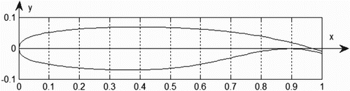
This study focuses on the buffet load of the NASA SC(2)-0714 supercritical airfoil which was designed by the Langley Research Center in the United States (US). It has a thickness to chord ratio e/c=13.86%, which is located at 37% of the chord length away from the leading edge. Its maximum camber is 1.5%, which is located at four fifths of the chord length away from the leading edge. Its maximum camber is 1.50%, which is located at 80% of the chord from the leading edge. The airfoil profile geometry data is acquired from the UIUC web site (http://m-selig.ae.illinois.edu/ads/coord_database.html#Nhttp://m-selig.ae.illinois.edu/ads/coord_database.html#N) and the chord length of the airfoil is c = 1000 mm (Figure ).
Figure 1. Profile of the NASA SC(2)-0714 airfoil.
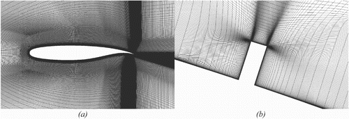
The transonic unsteady flow field around the NASA SC(2)-0714 supercritical airfoil with a microtab is simulated by solving the Navier–Stokes equations. The two-dimensional computational domain is divided by C-type structured girds with 129,821 nodes. The far-field boundaries are imposed at 50 times the chord length away from the profile. The length of the first layer mesh is 1 × 10⁻⁶c, and the first layer mesh point y+ is always less than 1. The grid resolution along the flow direction in the shock oscillation region is Δx/c ≈ 0.003 (where Δx is the average size of a single grid along the flow direction) and the grid resolution along the flow direction in the wake region near to the trailing edge is Δx/c ≈ 0.005 (Figure (a)). The grids around the microtab are locally refined (Figure (b)).
Figure 2. Flow field mesh division: (a) grids around the airfoil and (b) grids around the microtab.
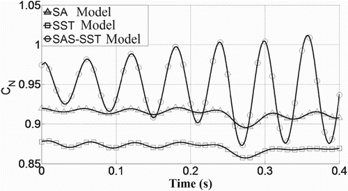
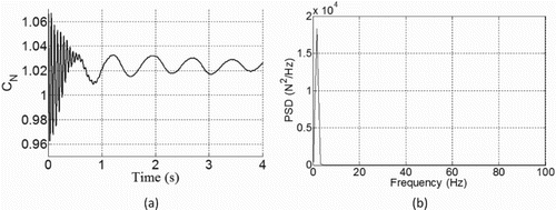
URANS simulations which use a one-equation turbulence model – such as the Spalart-Allmaras model (Spalart & Allmaras, Citation1992) – or a two-equation turbulence model – such as the k–ω shear stress transport model (Menter, Citation1994) – only generate large-scale unsteadiness, resulting in either a steady flow or a much lighter unsteady flow. However, the scale adaptive simulation-shear stress transport (SAS-SST) model (Menter & Egorov, Citation2005) can be dynamically adjusted to resolve structures in URANS simulations. This leads to an large eddy simulation-like behavior in the unsteady regions of the flow field and enables the turbulent spectrum to develop in the detached regions. Meanwhile, this model provides the standard Reynolds-averaged Navier–Stokes (RANS) capabilities in the stable flow regions. Hence, the SAS-SST model is suitable for the simulation of a developed buffet flow field (Figure ). The spatial flux terms and viscosity terms are discretized using a second-order accurate upwind finite-volume scheme which is modified from the one-order accuracy upwind scheme of Barth and Jespersen (Citation1989). The discretization of unsteady terms is based on the second-order accuracy backward Euler difference scheme, and the marching time step is 5 × 10⁻⁵ s. The Reynolds number, based on the free stream velocity and the chord length, is 15 × 106, and the free stream Mach number M∞ is set as 0.725, with the angle of incidence α = 3.5°, which is greater than the buffet onset angle of incidence αB = 3.0° (Bartels & Edwards, Citation1997; Jenkins, Citation1989).
Figure 3. Time history of the normal force coefficients obtained by different turbulence models.
Firstly, the simulation accuracy of the numerical method adopted to simulate the transonic unsteady flow field around the NASA SC(2)-0714 supercritical airfoil is validated via comparison with the results of an existing wind tunnel test (Bartels & Edwards, Citation1997; Jenkins, Citation1989). The conditions of the flow field are set as M∞ = 0.725, α = 3.0°, and Re = 15 × 106. In order to compare the buffet load frequency at different free stream velocities and between different airfoil chord lengths, the reduced frequency k (Equation (1)) is generally adopted:
(1)
where f is the frequency of buffet load, c is the chord length of the airfoil, and u is the free stream velocity.
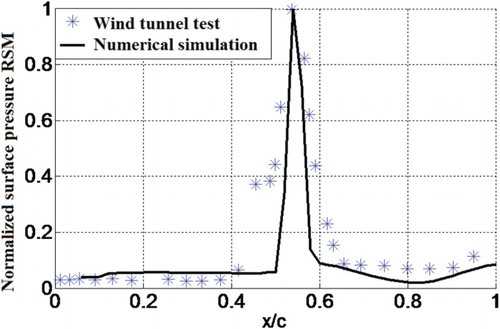
For the NASA SC(2)-0714 airfoil, the reduced frequency obtained by the numerical simulation is k = 0.22, which is very close to the value of k = 0.21 acquired from the test conducted by Bartels and Edwards (Citation1997). The time-averaged pressure distribution on the airfoil surface and the normalized pressure fluctuation root mean square value on the upper airfoil surface are obtained by numerical method and compared with the results of wind tunnel tests (Figures and ). The comparison shows that the numerical simulation results are in good agreement with the test results on the whole, with the exception that the numerical method slightly underestimates the range of the shock oscillation.
Figure 4. Time-averaged airfoil surface pressure distribution. Note: Wind tunnel data taken from Bartels et al. (Citation1997).
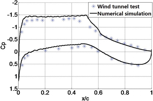
Figure 5. Normalized pressure fluctuation root mean square value. Note: Wind tunnel data taken from Bartels et al. (Citation1997).
3. Results and discussion
3.1. The characteristics of the flow field and buffet load for the baseline airfoil
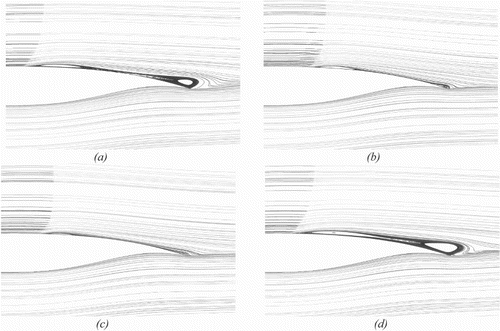
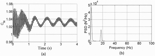
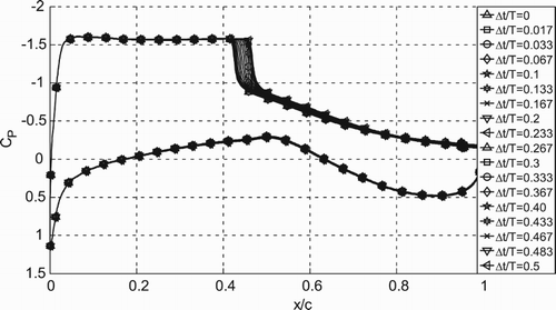
In order to determine the influence of the microtab on the flow field and buffet load of the NASA SC(2)-0714 airfoil, the main characteristics of the flow field and information on the buffet load at the flow condition, M∞ = 0.725, α = 3.5°, Re = 15 × 106, are presented so as to provide a base of reference. The range of the shock oscillation on the baseline airfoil (airfoil without microtab) is about 10.00% of the chord length (Figure ), the fluctuation magnitude of the normal force is about 14.60% of the normal force magnitude (Figure ), the reduced frequency of the normal force fluctuation is k = 0.22, and the corresponding fluctuation frequency of normal force is 17.38 Hz. Figure illustrates the streamlines around the airfoil when the shock arrives at the upstream and downstream turning points (the most upstream and downstream positions that the shock can reach in a shock oscillation cycle) and also shows the flow separation after the shock in the slightest and most serious condition respectively.
Figure 6. Pressure distribution on the baseline airfoil surface at different moments.
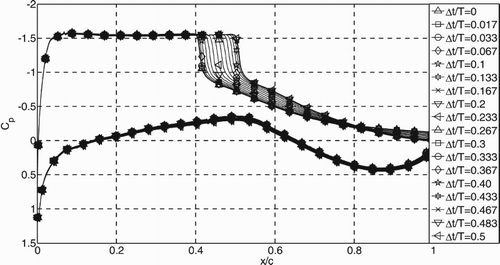
Figure 7. Time history of the normal force coefficient of the baseline airfoil.
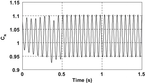
Figure 8. Streamlines behind the shock on the baseline airfoil for: (a) the shock at the upstream turning point, (b) the shock at the downstream turning point, (c) the flow separation for the least serious condition, and (d) the flow separation for the most serious condition.
3.2. The influence of the installation location of the microtab on the buffet load and flow field characteristics
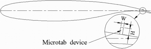
In order to investigate the effect of the installation location of the microtab on the buffet load and the characteristics of shock oscillation, the microtab was installed on the upper surface of the NASA SC(2)-0714 airfoil at four different positions: x/c = 0.6, x/c = 0.7, x/c = 0.8 and x/c = 0.9. The microtab is installed on an axis vertical to the airfoil surface and has a rectangular profile with a height of H/c = 0.50% and a width of W/c = 0.20%, where H is the absolute height of the microtab over the airfoil surface and W is the width of the microtab in the direction of airflow (Figure ).
Figure 9. Sketch of the microtab installed on the upper airfoil surface.
3.2.1. Microtab installation at x/c = 0.6 chord-wise on the upper airfoil surface
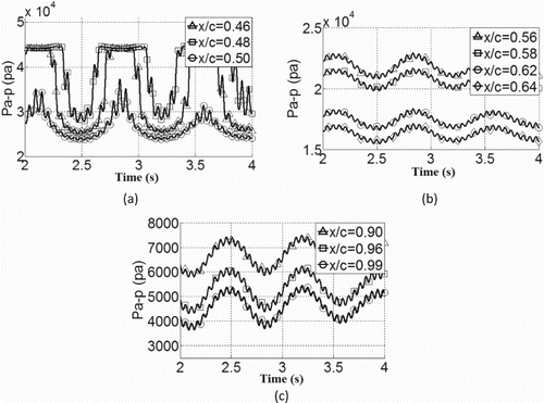
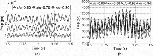
The flow field around the airfoil with the microtab installed at x/c = 0.6 chord-wise on the upper airfoil surface shows that the shock oscillates with a small amplitude and a high frequency and is simultaneously accompanied by an oscillation of a large amplitude and a low frequency. The high frequency of the shock oscillation is 17.38 Hz, which is the same as that of the shock oscillation on the baseline airfoil, while the low frequency is 1.58 Hz. Due to the interaction between the shock and the boundary layer, the flow variation within the boundary layer after the shock has a tendency similar to that of the shock oscillation (Figures and ). As a result, the pressure on the airfoil surface fluctuates with two frequencies in the regions after the shock (Figure ). It is obvious that the separated vortices after the shock, the separated vortices before and after the microtab and the separated vortices near the trailing edge of the airfoil always exist within a shock oscillation cycle.
Figure 10. Streamlines behind the shock on the airfoil with a microtab of protruding height H/c = 0.50% installed at x/c = 0.6 chord-wise on the upper airfoil surface (the shock oscillating near the upstream reverse point in a large-amplitude, low-frequency shock oscillation period) for: (a) the shock at the upstream turning point, (b) the middle moment during the shock traveling downstream, (c) the shock at the downstream turning point, and (d) the middle moment during the shock traveling upstream.
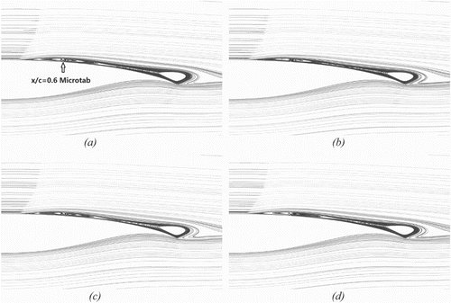
Figure 11. Streamlines behind the shock on the airfoil with a microtab of protruding height H/c = 0.50% installed at x/c = 0.6 chord-wise on the upper airfoil surface (the shock oscillating near the downstream reverse point in a large-amplitude, low-frequency shock oscillation period) for: (a) the shock at the upstream turning point, (b) the middle moment during the shock traveling downstream, (c) the shock at the downstream turning point, and (d) the middle moment during the shock traveling upstream.
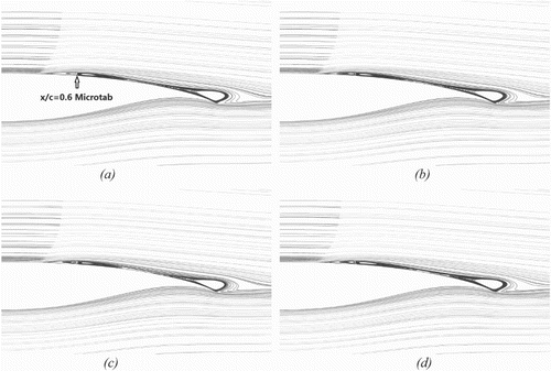
Figure 12. Pressure fluctuations over time on the upper airfoil surface for: (a) the region of shock oscillation, (b) the region near the microtab, and (c) the region near the trailing edge of the airfoil.
As the transonic buffet load mainly results from the shock oscillation, the magnitude of the buffet load depends on the shock oscillation range, i.e., the greater the shock oscillation range, the greater the buffet load, and vice versa. Figures (a) and (b) illustrate the chord-wise shock oscillating range in a large-amplitude, low-frequency cycle and a small-amplitude, high-frequency cycle, respectively. Compared with the shock oscillation range of the baseline airfoil (Figure ), the shock oscillation range on the airfoil with a microtab at x/c = 0.6 chord-wise is reduced by about 50%.
Figure 13. Pressure distribution on the airfoil surface for: (a) a large-amplitude, low-frequency cycle and (b) a small-amplitude, high-frequency cycle.
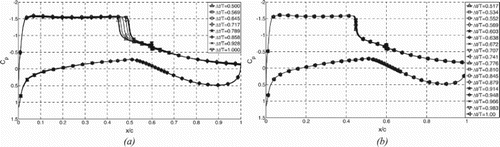
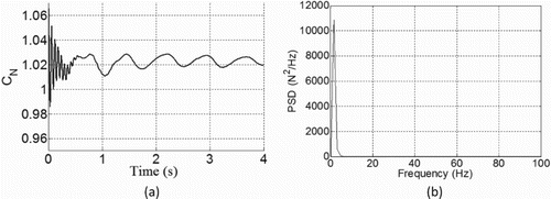
Figure (a) shows the time history of the normal force coefficient on the airfoil with a microtab at x/c = 0.6 chord-wise. Compared with the baseline airfoil, the fluctuation of normal force on the airfoil has two frequency components rather than a single frequency. The amplitude of normal force on the airfoil with a microtab at x/c = 0.6 chord-wise is reduced to 15% of that on the baseline airfoil. The power spectral density of the normal force is illustrated in Figure (b), which shows that the high-frequency fluctuation of normal force is 17.38 Hz, which is the same as that of the baseline airfoil. This demonstrates that the low-frequency fluctuation is induced by the microtab and dominates the normal force.
Figure 14. Characteristics of the normal force on the airfoil with a microtab installed at x/c = 0.6 chord-wise on the upper airfoil surface: (a) the normal force coefficient over time and (b) the power spectral density (PSD) of the normal force.
3.2.2. Microtab installations at x/c = 0.7 and x/c = 0.8 chord-wise on the upper airfoil surface
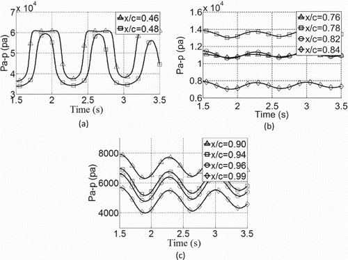
When the microtab is installed at x/c = 0.7 or x/c = 0.8 chord-wise on the upper airfoil surface, the shock oscillates and the scale of the vortices varies with a single frequency of 1.58 Hz, which is the same as the low frequency of shock oscillation on the airfoil with a microtab at x/c = 0.6 chord-wise. The behavior of the shock oscillation and scale of the vortex variation cause the surface pressure to fluctuate at the same frequency of 1.58 Hz (Figures and ).
Figure 15. Pressure fluctuations over time on the airfoil with a microtab installed at x/c = 0.7 chord-wise on the upper airfoil surface for: (a) the region of shock oscillation, (b) the regions near the microtab, and (c) the region near the trailing edge of the airfoil.
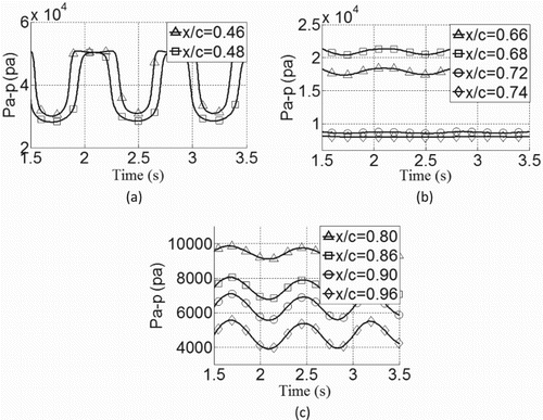
Figure 16. Pressure fluctuations over time on the airfoil with a microtab installed at x/c = 0.8 chord-wise on the upper airfoil surface for (a) the region of shock oscillation, (b) the regions near the microtab, and (c) the region near the trailing edge of the airfoil.
The differences in the flow fields between the airfoil with a microtab at x/c = 0.7 and the airfoil with a microtab at x/c = 0.8 are mainly manifested in the following respects. Firstly, there are two separated vortices after the microtab installed at x/c = 0.7 chord-wise on the upper airfoil surface within one shock oscillation cycle, while there is just a single separated vortex after the microtab installed at x/c = 0.8 chord-wise (Figures and ). Secondly, the shock oscillation range on the airfoil with a microtab installed at x/c = 0.7 chord-wise is almost 20% larger than that of the airfoil with a microtab installed at x/c = 0.8 chord-wise (Figure ). As a consequence, the amplitude of the normal force on the airfoil with a microtab installed at x/c = 0.8 chord-wise is 36% less than that of the airfoil with a microtab installed at x/c = 0.7 chord-wise (Figures (a) and (a)), and it is only 7% of that of the baseline airfoil. Because the flow fields around these two airfoils vary with the same frequency, the fluctuation frequency of the normal forces on both of these airfoils is equal to1.58 Hz (Figures (b) and (b)).
Figure 17. Streamlines behind the shock on the airfoil with a microtab of protruding height H/c = 0.50% installed at x/c = 0.7 chord-wise on the upper airfoil surface for: (a) the shock at the downstream turning point, (b) the middle moment during the shock traveling upstream, (c) the shock at upstream turning point, and (d) the middle moment during shock traveling downstream.
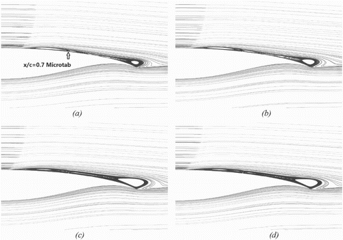
Figure 18. Streamlines behind the shock on the airfoil with a microtab of protruding height H/c = 0.50% installed at x/c = 0.8 chord-wise on the upper airfoil surface for: (a) the shock at the downstream turning point, (b) the middle moment during the shock traveling upstream, (c) the shock at upstream turning point, and (d) the middle moment during shock traveling downstream.
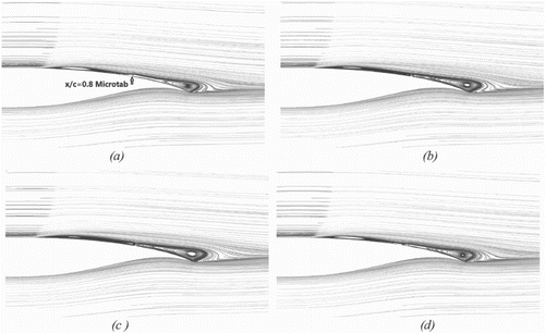
Figure 19. Pressure distribution on the surface of the airfoil with a microtab installed chord-wise on the upper airfoil surface at: (a) x/c = 0.7 and (b) x/c = 0.8.
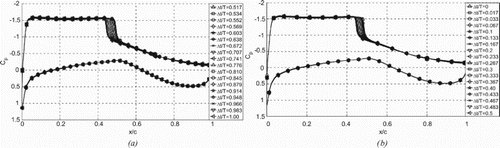
Figure 20. Characteristics of the normal force on the airfoil with a microtab installed at x/c = 0.7 chord-wise on the upper airfoil surface: (a) the normal force coefficient over time and (b) the power spectral density (PSD) of the normal force.
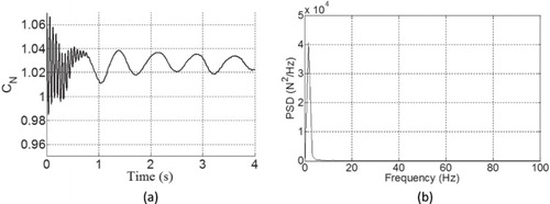
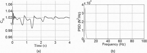
Figure 21. Characteristics of the normal force on the airfoil with a microtab installed at x/c = 0.8 chord-wise on the upper airfoil surface: (a) the normal force coefficient over time and (b) the power spectral density (PSD) of the normal force.
3.2.3. Microtab installation at x/c = 0.9 chord-wise on the upper airfoil surface
Compared with the airfoils with a microtab installed at x/c = 0.6, x/c = 0.7 and x/c = 0.8 chord-wise, the transonic unsteady flow field around the airfoil with a microtab installed at x/c = 0.9 presents a new flow pattern. There are two vortices in the region between the shock and the microtab, and the interaction mechanism between the shock and the boundary layer is similar to that seen with the baseline airfoil (Figures and ). Nevertheless, due to the interference effect produced by the microtab installed at x/c = 0.9 chord-wise, the interaction between the vortices before and behind the microtab have an evident impact on the flow field. The range of the shock oscillation and the amplitude of the vortex scale change after shock shows periodical variation (Figures –). The variation characteristics of the flow field around the airfoil with a microtab installed at x/c = 0.9 chord-wise makes the amplitude of fluctuation of the surface pressure on the upper airfoil surface vary periodically (Figures and ).
Figure 22. Streamlines behind the shock on the airfoil with a microtab installed at x/c = 0.9 chord-wise on the upper airfoil surface when the shock oscillation range is at minimum for: (a) the shock at the downstream turning point, (b) the middle moment during the shock traveling upstream, (c) the shock at upstream turning point, and (d) the middle moment during shock traveling downstream.
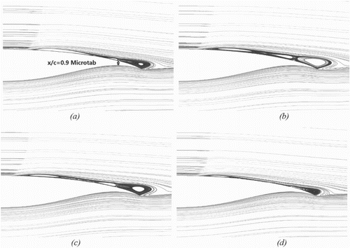
Figure 23. Pressure distribution on the surface of the airfoil with a microtab installed at x/c = 0.9 chord-wise on the upper airfoil surface when: (a) the shock oscillation range is at minimum and (b) the shock oscillation range is at maximum.
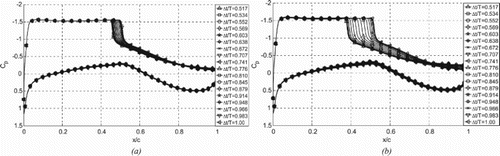
Figure 24. Streamlines behind the shock on the airfoil with a microtab installed at x/c = 0.9 chord-wise on the upper airfoil surface when the shock oscillation range is at maximum for: (a) the shock at the downstream turning point, (b) the middle moment during the shock traveling upstream, (c) the shock at upstream turning point, and (d) the middle moment during shock traveling downstream.
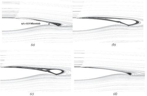
Figure 25. Pressure fluctuations over time in the shock oscillation regions on the airfoil with a microtab installed at x/c = 0.9 chord-wise on the upper airfoil surface when: (a) the shock oscillation range is at minimum and (b) the shock oscillation range is at maximum.
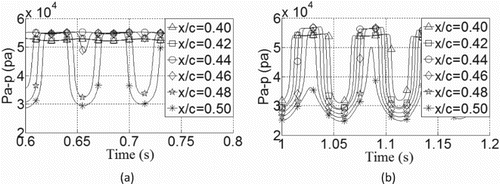
Figure 26. Pressure fluctuations over time on the airfoil with a microtab installed at x/c = 0.9 chord-wise on the upper airfoil surface for: (a) the regions between the shock and the trailing edge and (b) the regions near the microtab.
The fluctuation frequency of the normal force on the airfoil with a microtab installed at x/c = 0.9 chord-wise on the upper surface is the same as that of the baseline airfoil (Figure (b)), but the amplitude of the normal force varies periodically with time (Figure (a)) and the variation frequency of the normal force fluctuating amplitude is 1.58 Hz. The minimal normal force amplitude is 66% of that of the baseline airfoil, and the maximal normal force amplitude is 134% of that of the baseline airfoil.
Figure 27. Characteristics of the normal force on the airfoil with a microtab installed at x/c = 0.9 chord-wise on the upper foil surface for: (a) the normal force coefficient over time and (b) the power spectral density (PSD) of the normal force.
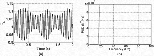
Figure 28. Streamlines behind the shock at on the airfoil with a microtab of protruding height H/c = 0.75% installed at x/c = 0.8 chord-wise on the upper airfoil surface for: (a) the shock at the downstream turning point, (b) the middle moment during the shock traveling upstream, (c) the shock at upstream turning point, and (d) the middle moment during shock traveling downstream.
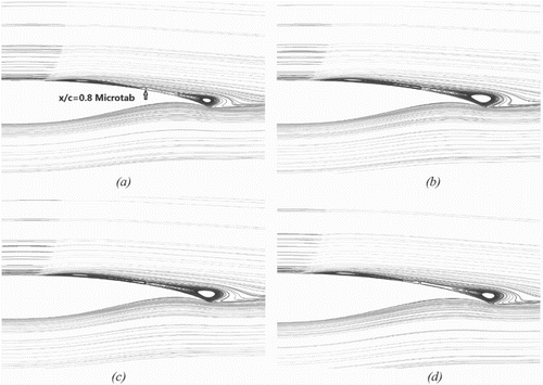
Figure 29. Pressure distribution on the surface of the airfoil with a microtab of protruding height H/c = 0.75%.
3.3. The influence of the microtab protruding height on the buffet load and flow field characteristics
Through analyzing the buffet load and the characteristics of the flow field around the NASA SC(2)-0714 airfoil with a microtab installed at different chord-wise positions on the upper surface, it was found that the buffet load can be alleviated by a microtab installed at x/c = 0.6, x/c = 0.7 or x/c = 0.8 chord-wise. However, the microtab installed at x/c = 0.8 chord-wise provides the best buffet load alleviation of the three positions. Therefore, in exploring the effects of the protruding height of the microtab on the buffet load and the flow field, the microtab was fixed at the position of x/c = 0.8. The flow fields around the airfoils with microtabs of protruding heights H/c = 0.50%, H/c = 0.75% and H/c = 1.00% were numerically simulated.
The characteristics of the flow field around the airfoils with microtabs of protruding heights H/c = 0.50% and H/c = 0.75% are very similar, the only difference being the shock oscillation range and the amplitude of the vortex scale change (, (b), and ). The amplitude of the normal force of the airfoil with a microtrab of protruding height H/c = 0.75% is 15% less than that of the airfoil with a microtrab of protruding height H/c = 0.50%. The variation time histories of flow fields around these two airfoils present a stable and slow attenuation, and this flow field variation tendency cause the surface pressure fluctuations on the upper airfoil surface and the normal force to present the same trend (Figures and ). However, there is a clear difference in the time history of the flow field variation between the airfoil with a microtrab of protruding height H/c = 1.00% and the other two.
Figure 30. Pressure fluctuations over time on the airfoil with a microtab of protruding height H/c = 0.75% installed at x/c = 0.8 chord-wise on the upper airfoil surface for: (a) the shock oscillation region, (b) the middle region between the shock and the trailing edge, and (c) the regions near the microtab.
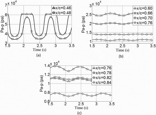
Figure 31. Characteristics of the normal force on the airfoil with a microtab of protruding height H/c = 0.75% installed at x/c = 0.8 chord-wise on the upper airfoil surface: (a) the normal force coefficient over time and (b) the power spectral density (PSD) of the normal force.
The time history of the flow field variation around the airfoil with a microtrab of protruding height H/c = 1.00% can be divided into two stages. The first can be called the ‘disturbance stage’ as the variation amplitude of the flow field after the shock increases with time, and this variation tendency causes the amplitude of the surface pressure fluctuation and normal force to increase (Figures and ). In the second stage, the variation amplitude of the flow field decays rapidly with time but the variation frequency of the flow field remains constant, a variation tendency which makes the amplitude of the surface pressure fluctuation and normal force decrease with time, so the second stage can be referred to as the ‘amplitude attenuation stage’.
Figure 32. Pressure fluctuations over time on the airfoil with a microtab of protruding height H/c = 1.00% installed at x/c = 0.8 chord-wise on the upper airfoil surface for: (a) the shock oscillation region, (b) the middle region between the shock and the trailing edge, and (c) the regions near the microtab.
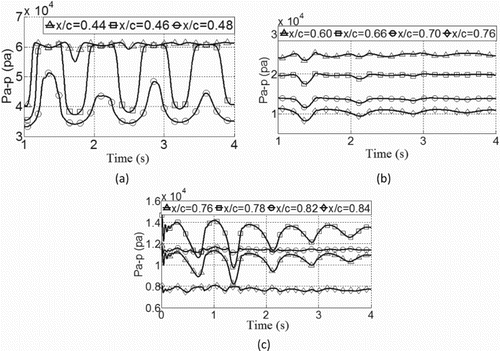
Figure 33. Characteristics of the normal force on the airfoil with a microtab of protruding height H/c = 1.00% installed at x/c = 0.8 chord-wise on the upper airfoil surface: (a) the normal force coefficient over time and (b) the power spectral density (PSD) of the normal force.
3.4. Discussion on the mechanism of buffet load alleviation
The microtabs installed at x/c = 0.6, x/c = 0.7 and x/c = 0.8 chord-wise on the upper airfoil surface cause a change in the expanding modes of the vortices. Furthermore, because the intensity of the interaction between the shock and vortices before the microtab is greater than the intensity of the interaction between the vortices after the microtab and the airflow above these vortices, the intensity variation of the vortices after the microtab lags behind that of the vortices before the microtab. Hence, there is a height difference between the vortices before and after the microtab (Figure ), which forms a ‘geometry effect’ (Iovnovich & Raveh, Citation2012). This geometry effect causes the velocity variation tendency of the flow after the microtab and above the vortices to be contrary to that caused by the interaction between the shock and the boundary layer, and this weakens the interaction intensity between the vortices after the microtab and the flow above these vortices. Therefore, the variation amplitude and the change rate of the vortex intensity after the microtab decrease substantially. The intensity variation of the vortices after the microtab influence the circulation of the airfoil, and this circulation variation affects the shock intensity, so the shock intensity variation amplitude and rate decrease dramatically, and thus the interaction intensity between the shock and the boundary layer decreases. Consequently, the shock oscillation range and moving speed decrease, and as a result the fluctuation amplitude and frequency of the buffet load also decrease.
Figure 34. The states of the vortices before and after the microtab for the shock and the boundary layer for: (a) the interaction during the strengthening stage and (b) the interaction during the weakening stage.

The interaction behaviors between the shock and the boundary layer are different when the microtab is installed on the upper airfoil surface at x/c = 0.6, x/c = 0.7, x/c = 0.8 and x/c = 0.9 chord-wise. A stable and new mode of interaction between the shock and the boundary layer is formed on these airfoils. This interaction mode is named the microtab mode, and the mode of interaction between the shock and the boundary layer that occur on the baseline airfoil is referred to as the baseline mode. The two modes have their own shock wave oscillation frequencies.
When the microtab is installed at x/c = 0.6 chord-wise, the shock oscillation and vortex intensity variation have two different frequencies due to the existence of two modes of interaction between the shock and the boundary layer on the airfoil simultaneously – that is, the microtab mode and baseline mode exist simultaneously. However, only the microtab mode exists on the airfoil when the microtab is installed at x/c = 0.7 or x/c = 0.8 chord-wise – and when the microtab is installed at x/c = 0.9 chord-wise, the baseline mode plays a predominant role, while the microtab mode plays a disturbance role in the unsteady flow around the airfoil.
4. Conclusion
This paper has presented an investigation of the influence of microtab devices on the characteristics of the buffet load and shock oscillation to which the NASA SC(2)-0714 supercritical airfoil is subjected in transonic air flow. The unsteady flow field was simulated using a URANS method with an SAS-SST turbulence model. The effect of the installation location of the microtab on the buffet load and the characteristics of the flow field was investigated by installing the microtab on the upper surface of the airfoil at x/c = 0.6, x/c = 0.7, x/c = 0.8 and x/c = 0.9 chord-wise. Based on the time history of the normal force and the characteristics of the shock oscillation, it is concluded that the shock oscillation range and the amplitude of the buffet load decrease when the microtab is installed at x/c = 0.7 or x/c = 0.8. This positioning can also decrease the average moving speed of the shock and hence decrease the buffet load fluctuation frequency. The effect of the microtab height protruding from the airfoil surface on the buffet load was also studied with the microtab installed at x/c = 0.8 chord-wise on the upper surface of the airfoil. The results indicate that the buffet load alleviation efficiency is best for a microtab with a protruding height of H/c = 0.75% compared to the other heights that were tested. Finally, the mechanism of microtab buffet load alleviation was presented. The height difference between the vortices before and after the microtab causes the velocity variation tendency of the flow after the microtab and above the vortices to be contrary to that caused by the interaction between the shock and the boundary layer. This change can suppress the shock oscillation and alleviate the buffet load of the NASA SC(2)-0714 airfoil. The influence of a span-wise arrangement scheme of microtabs on the developed buffet flow field and buffet load of a wing is left to future work.
Acknowledgments
The authors would like to gratefully acknowledge Dr. Huixue Dang of the Chang’an University and Yan Ouyang of the Northwestern Polytechnical University for their discussions and suggestions for this study.
Disclosure statement
No potential conflict of interest was reported by the authors.
Additional information
Funding
References
- Baker, J. P., Standish, K. J., & Van Dam, C. P. (2007). Two-dimensional wind tunnel and computational investigation of a microtab modified airfoil. Journal of Aircraft, 44(2), 563–572. doi: 10.2514/1.24502
- Bartels, R. E., & Edwards, J. W. (1997). Cryogenic tunnel pressure measurements on a supercritical airfoil for several shock buffet conditions (Report, National Aeronautics and Space Administration). Langley Research Center, USA.
- Barth, T. J., & Jespersen, D. C. (1989). The design and application of upwind schemes on unstructured meshes. 27th Aerospace Sciences Meeting, January 1989, Reno Nevada, USA, AIAA 89-0366.
- Caruana, D., Corrège, M., & Reberga, O. (2000). Buffet and buffeting active control. Fluids 2000, June 2000, Denver CO, USA, AIAA 2000-2069.
- Chow, R., & Dam, C. P. V. (2006). Unsteady computational investigations of deploying load control microtabs. Journal of Aircraft, 43(5), 1458–1469. doi: 10.2514/1.22562
- Gibb, J. (1988). The cause and cure of periodic flows at transonic speed. Cranfield: Cranfield Institute of Tech.
- Iovnovich, M., & Raveh, D. E. (2012). Reynolds-averaged Navier–Stokes study of the shock-buffet instability mechanism. AIAA Journal, 50(4), 880–890. doi: 10.2514/1.J051329
- Jenkins, V. R. (1989). NASA SC(2)-0714 airfoil data corrected for sidewall boundary-layer effects in the Langley 0.3-meter transonic cryogenic tunnel (NASA Technical Paper 2890). Langley Research Center, USA.
- König, B., Pätzold, M., & Lutz, T. (2009). Numerical and experimental validation of three-dimensional shock control bumps. Journal of Aircraft, 46(2), 675–682. doi: 10.2514/1.41441
- Mayda, E. A., Van Dam, C. P., & Yen-Nakafuji, D. (2005). Computational investigation of finite width microtabs for aerodynamic load control. 43rd AIAA Aerospace Sciences Meeting and Exhibit, 2005, Reno Nevada, USA, AIAA 2005-1185.
- Menter, F. R. (1994). Two-equation eddy-viscosity turbulence models for engineering applications. AIAA Journal, 32(8), 1598–1605. doi: 10.2514/3.12149
- Menter, F. R., & Egorov, Y. (2005). A scale-adaptive simulation model using two-equation models. 43rd AIAA Aerospace Sciences Meeting and Exhibit, January 2005, Reno Nevada, USA, AIAA 2005-1095.
- Molton, P., Dandois, J., Lepage, A., Brunet, V., & Bur, R. (2013). Control of buffet phenomenon on a transonic swept wing. AIAA Journal, 51(4), 761–772. doi: 10.2514/1.J051000
- Obert, E. (2009). Aerodynamic design of transport airplane. Amsterdam: IOS Press BV.
- Ogawa, H., Babinsky, H., & Pätzold, M. (2008). Shock-wave/boundary-layer interaction control using three- dimensional bumps for transonic wings. AIAA Journal, 46(6), 1442–1452. doi: 10.2514/1.32049
- Spalart, P. R., & Allmaras, S. R. (1992). A one-equation turbulence model for aerodynamic flows. 30th Aerospace Sciences Meeting and Exhibit, January 1992, Reno NV, USA, AIAA 92-0439.
- Unal, U. O., & Goren, O. (2011). Effect of vortex generators on the flow around a circular cylinder: Computational investigation with two-equation turbulence models. Engineering Applications of Computational Fluid Mechanics, 5(1), 99–116. doi: 10.1080/19942060.2011.11015355